A Novel Hierarchical Optimal Scheduling and Coordination Control Method for Microgrid Based on Multi-Energy Complementarity

Abstract

To address the uncertainty of intermittent energy sources and enhance the economic efficiency and operational performance of microgrids, this paper proposes a novel three-layer coupled microgrid scheduling model based on the principles of model predictive control, optimized and solved using an improved dung beetle algorithm. Firstly, by comprehensively considering time-varying electricity prices and pollution protection costs, the model optimizes and mitigates the impact of uncertain factors in day-ahead scheduling, thereby constructing a new three-layer scheduling framework. Secondly, improvements to the traditional dung beetle algorithm, including population initialization, rolling behavior, and foraging behavior, are validated through simulations, demonstrating enhanced accuracy and convergence speed. Furthermore, the improved dung beetle algorithm is utilized to optimize the economic performance of the scheduling layer, determining optimal controls within the rolling control framework. Finally, through economic comparisons, rolling scheduling analysis, and control effectiveness experiments, this study demonstrates that the proposed model and algorithm significantly improve the environmental economics of microgrids while enhancing system controllability and stability.

1. Introduction

Microgrids are small-scale power distribution systems composed of various components, facilitating the efficient utilization of renewable energy while enhancing the flexibility and reliability of power systems, thus promoting the optimization of energy structures and sustainable development. In recent years, the global energy transition has accelerated, driven by decarburization goals and the rapid growth of distributed renewable energy sources (RES). As a key enabler of localized energy management, the microgrid has gained significant attention for its ability to integrate RES, improve grid resilience, and support energy access in remote areas [1]. Governments worldwide have also prioritized microgrid deployment through policies such as renewable portfolio standards, carbon pricing mechanisms, and subsidies for smart grid technologies [2]. However, the uncertainty associated with intermittent distributed energy sources and load demands leads to significant forecasting errors in day-ahead scheduling, resulting in continuously varying output from generation units and difficulty in adjusting to these changes. These challenges are further amplified by dynamic energy policies that emphasize both economic efficiency and environmental sustainability. Therefore, addressing the uncertainties of intermittent distributed energy and load demands remains a critical challenge in optimizing microgrid scheduling [3].

Model predictive control (MPC), based on rolling optimization and feedback correction principles, effectively manages uncertainty, flexibly handles multiple constraints, and tracks various optimization objectives. As a result, MPC has found widespread application in microgrid optimization, addressing uncertainties related to renewable energy, load demands, and market electricity price fluctuations [3,4].

In reference [5], a day-ahead economic scheduling strategy for microgrids was developed to address uncertainties in renewable energy and load forecasting, while reference [6] proposed a distributed economic model predictive control (DEMPC) strategy integrated with a model-based intrusion detection unit and event-triggering mechanism to counter cyber-attacks and reduce computational burdens in load frequency regulation with large-scale plug-in electric vehicle participation. However, in microgrid scheduling, traditional centralized model predictive control faces challenges such as high online computation requirements and poor scalability when dealing with complex problems. This makes it difficult to apply traditional MPC to integrated energy systems with many distributed units, especially in scenarios requiring high real-time performance and flexibility. Consequently, an increasing number of studies have leaned towards using hierarchical architectures to address scheduling issues in microgrids [7]. References [8,9] proposed and implemented a day-ahead to intraday architecture. In the day-ahead phase, an optimal cost scheduling model is constructed, while the intraday phase employs MPC for corrective control to manage uncertainties in renewable energy generation and load forecasting. This architecture improves system stability and economic efficiency through phased optimization. Additionally, the intelligent algorithms used in reference [10] enhanced the system’s response speed during model optimization and solving. However, the accuracy of predictive variables is inversely proportional to the prediction time [11], and as the prediction time extends, forecasting errors tend to increase, particularly in the later stages, which further exacerbates the prediction error [12] and affects the execution effectiveness of scheduling plans. Therefore, to enhance prediction accuracy and reduce forecasting errors, optimization of the intraday scheduling strategy is necessary. Reference [13] proposed an intraday hierarchical model predictive scheme combining optimization, hierarchy, and iterative control concepts, but this research primarily focused on photovoltaic cluster systems and did not sufficiently consider the impacts of multi-source power supply and energy storage systems. Reference [14] introduced a three-layer architecture for multi-source power supply, achieving more controllable and efficient optimization scheduling. However, the optimization scheduling and rolling solution did not utilize intelligent algorithms, and the computational load of cost-minimization optimization scheduling in the intraday layer proved too high to accommodate more detailed real-time control.

In summary, current research on three-layer scheduling models is relatively limited both domestically and internationally, and existing studies have not fully considered time-sharing tariffs and environmental protection costs; the convergence accuracy and convergence speed of intelligent algorithms in dealing with complex problems are unsatisfactory. Based on this, this paper proposes a three-layer optimization scheduling strategy based on an improved dung beetle algorithm. The first layer integrates time-varying electricity prices and environmental pollution costs, aiming for the economic operation of the microgrid and optimizing through the improved intelligent algorithm. The second layer addresses the operational efficiency of units, advancing optimization scheduling to the day-ahead phase, using the improved intelligent algorithm for rolling optimization to reduce uncertainties in day-ahead renewable energy and load forecasting. The third layer employs actual output values to provide feedback correction to the second layer, considering the operational speed of units and implementing online operations with the improved intelligent algorithm. Ultimately, the feasibility and superiority of the proposed strategy and algorithm are validated through comparative analysis of day-ahead scheduling economic algorithms and line-tracking effectiveness. The scheduling strategy proposed in this paper can solve the volatility problem caused by the uncertainty of renewable energy sources; the convergence speed and convergence accuracy of the proposed algorithm are significantly improved, which provides a tool for solving the complex optimization and solution problems.

Paper Organization

Before diving into the technical details, the following is an outline of the paper’s structure:

Section 1—Introduction: Provides background and motivation for the study.

Section 2—Construction of a Three-Layer Coordinated Scheduling Model: Describes the proposed three-layer hierarchical scheduling framework.

Section 3—Improvement of the Dung Beetle Optimization Algorithm: Discusses enhancements made to the traditional dung beetle optimizer (DBO) algorithm.

Section 4—Optimization and Solution of a Three-Layer Coordinated Optimal Scheduling Model Based on OTcmDBO: Presents the optimization process using the improved algorithm.

Section 5—Analysis and Verification of Numerical Examples: Validates the proposed model and algorithm through case studies.

Section 6—Conclusions: Summarizes the main findings and contributions of the study.

2. Construction of a Three-Layer Coordinated Scheduling Model

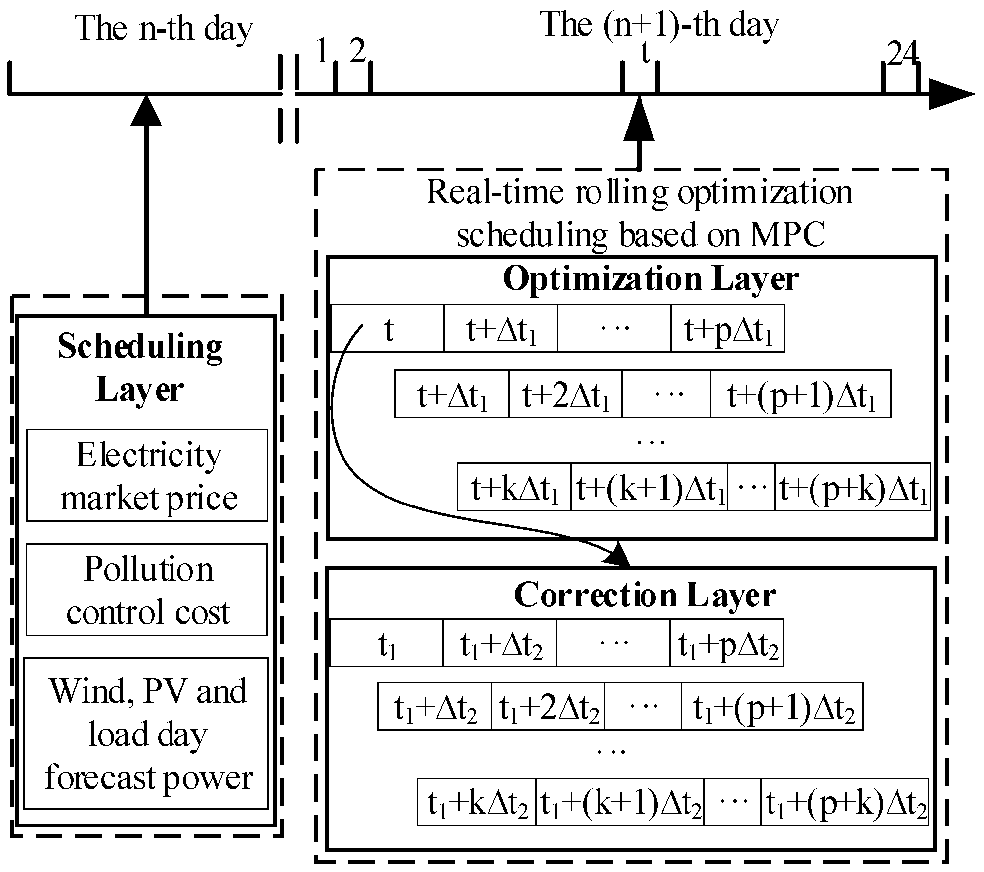
2.1. Three-Tier Coordinated Movement Control Framework

To effectively accommodate intermittent distributed energy sources in microgrids, this paper constructs a three-layer optimization scheduling model across multiple time scales, recognizing that forecasting errors for renewable energy and load decrease as prediction time shortens. The model comprises the first layer, the scheduling layer; the second layer, the optimization layer; and the third layer, the correction layer; as illustrated in Figure 1. The specific coordination and scheduling approach is as follows:

(a)

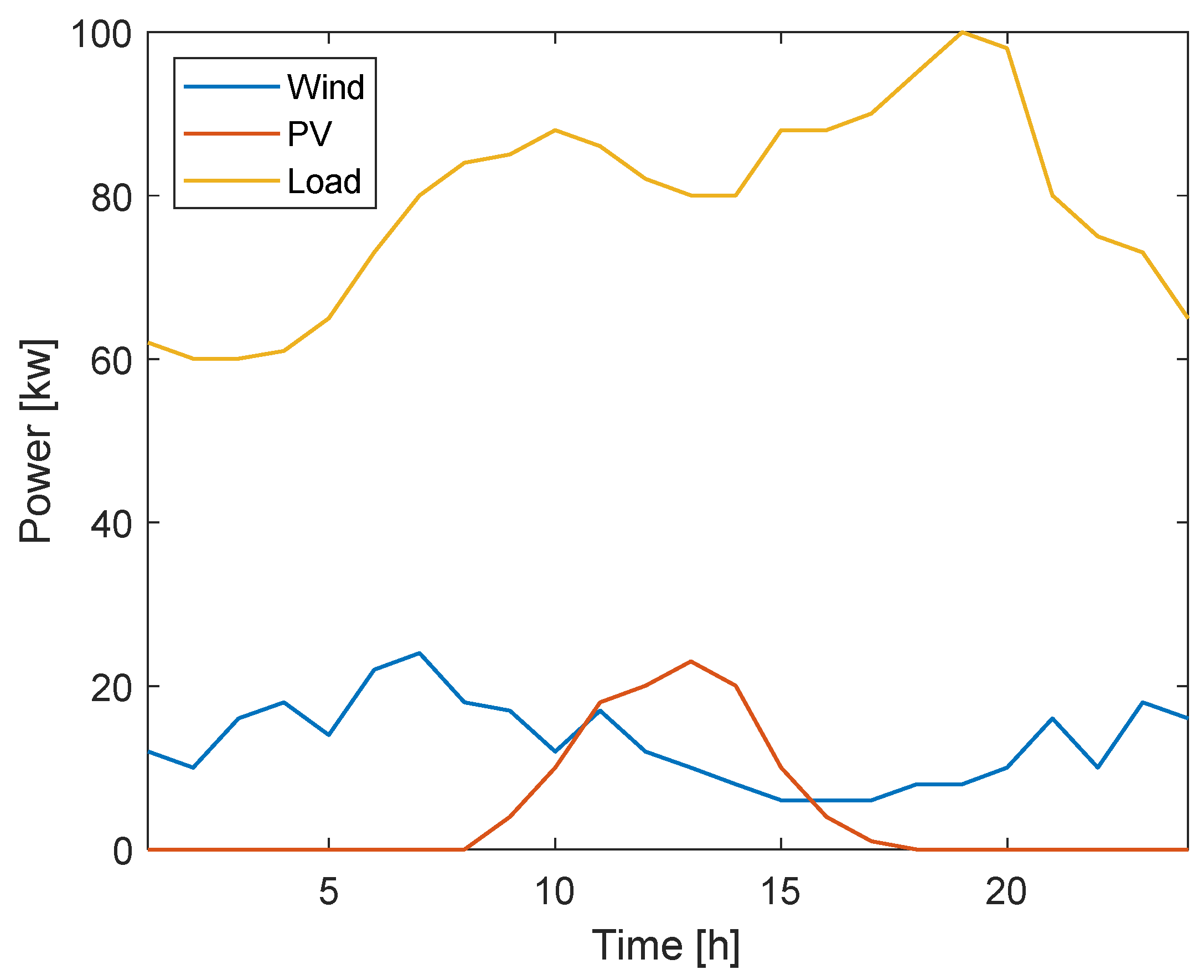
First Layer—Scheduling Layer: This layer operates on a “day-ahead” time scale and is based on forecasts of renewable energy and load demand. A 24 h planning cycle (Δt = 1 h) is defined at the dispatch level, covering the co-optimization of PV, wind turbines, storage (SOC 0.2–0.9), gas turbine, diesel generator, and grid interconnections. It comprehensively considers time-varying electricity prices and environmental management costs, aiming to minimize the system’s economic costs. By optimizing control variables such as micro-source power, charge, and discharge adjustments, and the output ratio of interconnection lines, a generation plan for each hour of the following day is established.

(b)

Second Layer—Optimization Layer: This layer functions on an “intraday” time scale, managing units according to the day-ahead generation plan. The optimization layer uses a 4 h rolling window (Δt = 15 min) to dynamically adjust the control variables: energy storage charging and discharging power, gas turbine, and diesel generator output power. The objective is to minimize tracking errors for the interconnection line power and the state of charge (SOC) of energy storage based on the day-ahead plan, solving for the optimal control sequence for each unit. The power state values of the units, energy storage, and interconnection lines derived from this sequence are then used as initial values for the next time segment in the optimization layer.

(c)

Third Layer—Correction Layer: This layer operates on a “real-time” time scale, using the scheduling values obtained from the optimization layer as a reference for the real-time management of units. The optimization cycle is refined into three periods, with rolling corrections occurring every 5 min. Using an MPC controller, the inputs of the system are gas turbine, diesel generator, and energy storage charging and discharging power. The output is the exchanged power of the contact line and the energy storage system. The objective function is to minimize the input variables by tracking the contact line power and the energy storage SOC day-ahead schedule value. A closed loop system is formed by the difference between the output power and the actual power as a feedback regulation.

Figure 1. Three-layer coordinated scheduling framework.

Figure 1. Three-layer coordinated scheduling framework.

The scheduling layer serves as the foundation for the optimization layer, providing an hourly generation plan. The optimization layer enhances the scheduling layer by significantly reducing the impact of uncertainties present in day-ahead planning. The correction layer is the ultimate goal of the optimization layer; it achieves online real-time control by performing feedback corrections on the optimized reference values based on actual output.

2.2. Construction of Scheduling Layer

The day-ahead optimization scheduling comprehensively considers time-varying electricity prices and pollution control costs. By reasonably planning the operating power of controllable micro-sources, optimizing energy storage charging and discharging, and allocating the power purchase and sale of the microgrid, the objective is to minimize the total cost of the system. The nonlinear features of the optimization model include that time-of-day tariffs have step-segmented function characteristics, pollution costs are quadratically related to power generation, storage charging and discharging efficiencies have asymmetric nonlinear constraints, and grid trading power is affected by threshold effects. Nonlinear terms are processed by introducing mixed integers. The objective function can be expressed as follows:

$$\begin{array}{ll}\min J_{\mathrm{ex}-\mathrm{d}}=& {\displaystyle \sum _{t=1}^T{\displaystyle \sum _{i=1}^N((C_{G\mathrm{i}-f}+C_{G\mathrm{i}-ma}+C_{G\mathrm{i}-pd})\ast P_{Gi}(t))}}\\ & +{\displaystyle \sum _{t=1}^T(C_b\ast P_b(t)+C_g\ast P_g(t)})\end{array}$$

(1)

In this model, J_ex−d represents the total economic cost of optimized scheduling over the total time period T, with N being the number of distributed energy sources. The costs include C_Gi−f, C_Gi−ma, and C_Gi−pd, which represent the fuel, maintenance, and pollution carbon emission costs, respectively, for each generation unit [15]. Additional costs include C_b, the maintenance cost of energy storage, and C_g, the price at which the microgrid buys or sells electricity to the main grid. Power variables such as P_Gi(t) (the power of each distributed energy source at time t), P_b(t) (the charging or discharging power of energy storage at time t), and P_g(t) (the power purchased or sold to the distribution network by the microgrid) are also integral to the model.

The day-ahead optimization scheduling must satisfy the following constraints:

(1)

Power balance constraint

$${\displaystyle \sum _{i=1}^N(P_{Gi}(t)+P_b(t)+P_g}(t))=P_{Load}(t)$$

(2)

Here, N is the total number of time slots, and P_Load(t) represents the load demand power at time t.

(2)

Distributed power constraints

$$P_{Gi-\min }\le P_{Gi}(t)\le P_{Gi-\max }$$

(3)

Here, P_Gi−min and P_Gi−max denote the minimum and maximum output power limits for the i-th distributed energy source, respectively.

(3)

Power climb constraint of distributed power supply

$$\Delta P_{Gi-\min }\le P_{Gi}(t)-P_{G\mathrm{i}}(t-1)\le \Delta P_{Gi-\max }$$

(4)

Here, ΔP_Gi−min and ΔP_Gi−max represent the minimum and maximum ramping power limits for the i-th distributed energy source, respectively.

(4)

Constraints on the transmission power of the tie line

$$P_{g-\min }\le P_g(t)\le P_{g-\max }$$

(5)

Here, P_g−min and P_g−max represent the minimum and maximum allowable transmission power of the interconnection line, respectively.

(5)

Capacity constraint of energy storage unit

The calculation formula for the state of charge is as follows:

$$SOC(t)=\left\{\begin{array}{l}SOC(t-1)-\eta {\displaystyle \frac{P_b(t)\ast \Delta t}{E_b}},P_b(t)\le 0\\ SOC(t-1)-{\displaystyle \frac{1}{\eta }}{\displaystyle \frac{P_b(t)\ast \Delta t}{E_b}},P_b(t)>0\end{array}\right.$$

(6)

Here, SOC(t) denotes the state of charge at time t, η represents the energy storage efficiency, P_b(t) is the charging or discharging power of the energy storage at time t, E_b is the battery capacity, and Δt is the time interval.

The constraints on the state of charge are as follows:

$$SO{C}_{\min }\le SOC(t)\le SO{C}_{\max }$$

(7)

Here, SOC_min and SOC_max represent the minimum and maximum limits of the state of charge capacity, respectively.

(6)

The constraints on the charging and discharging power of energy storage are as follows:

$$-P_{dis-\max }\le P_b(t)\le P_{ch-\max }$$

(8)

Here, P_dis−max and P_ch−max represent the maximum discharging and charging power of the energy storage system, respectively.

2.3. Construction of Optimization Layer and Correction Layer

The correction layer is built on the foundation of the optimization layer; thus, the two layers are integrated together. The scheduling process is illustrated in Figure 2. The optimization layer operates on a 15 min cycle, generating a scheduling plan for the next hour, while the correction layer functions on a 5 min cycle, producing a scheduling plan for the next 15 min. However, only the first value of the control sequence is executed during each cycle, ensuring that a control operation is performed only once per scheduling period to maintain system stability. The optimization layer is primarily responsible for formulating long-term scheduling plans and issuing them to the correction layer as reference values. The correction layer adjusts control variables based on the reference values from the optimization layer and real-time state information, allowing it to respond effectively to uncertainties. There is a feedback mechanism among the correction layer, optimization layer, and real-time status, facilitating updates to the initial state values at each time step.

To achieve effective real-time control and optimization of the microgrid, the optimization layer and correction layer are designed with specific objective functions and constraints. The optimization layer aims to minimize the tracking errors of the interconnection line power and the SOC of the energy storage system based on the day-ahead scheduling plan. This is achieved by formulating the following objective function:

$$\min J_{track}={\displaystyle \sum _{t=1}^N\left({\omega }_{tr1}{‖P_g(t)-P_{g,ref}(t)‖}^2+{\omega }_{tr2}{‖SOC(t)-SO{C}_{ref}(t)‖}^2\right)}$$

(9)

Here, P_g(t) and P_g,ref(t) are the actual and reference interconnection line powers at time t, respectively. SOC(t) and SOC_ref(t) are the actual and reference SOC values at time t, respectively. ω₁ and ω₂ are weighting factors that balance the importance of the two tracking errors.

The constraints for the optimization layer include power balance, distributed power limits, power climb constraints, tie line power limits, energy storage capacity limits, and charging/discharging power limits, as described in Section 2.2. The correction layer further refines the scheduling plan obtained from the optimization layer by conducting rolling corrections every 5 min. The objective function for the correction layer is similar to that of the optimization layer, but with a shorter prediction horizon to accommodate real-time changes.

The key motivation behind the design of these optimization functions is to ensure that the microgrid operates efficiently and stably by closely tracking the planned values while adhering to the operational constraints. This approach helps in reducing the impact of uncertainties from renewable energy sources and load demands.

Hierarchical model predictive control is an optimization framework for dealing with complex large-system control problems by means of hierarchical decomposition strategy, whose core idea is to disassemble the global control objective into multiple interrelated sub-problems, and to achieve overall optimization through the synergy of controllers at different hierarchical levels. In this paper, the input variables of the MPC controller are the power increments of gas turbine, diesel generator, and energy storage charging/discharging; the perturbation variables are the power increments of wind power, photovoltaic, and load demand; the objective function is to track the power of the contact line and the planned value of the storage SOC day-ahead to minimize the input variables; and finally, the difference between the output power and the actual power is used as the feedback regulation to constitute the closed-loop control.

Focusing on the establishment of the MPC rolling optimization scheduling model, the principles of the optimization layer and the correction layer are similar. Below, we will illustrate using the optimization layer as an example, without further elaboration on the correction layer.

Based on the dynamic characteristics of the microgrid, the power balance equation and the iterative equation of the state of charge are utilized. Let the state input vector be defined as x(t) = [P_MT(t), P_DE(t), P_b(t), SOC(t), P_g(t)]^T, the control variable vector as u(t) = [ΔP_MT(t), ΔP_DE(t), ΔP_b(t)]^T, the disturbance input vector as r(t) = [ΔP_WT(t), ΔP_PV(t), ΔP_Load(t)]^T, and the output variable vector as y(t) = [P_g(t), SOC(t)]^T.

Here, P_MT(t) represents the output power of the micro gas turbine, P_DE(t) denotes the output power of the diesel generator, and P_b(t) is the charging or discharging power of the energy storage. ΔP_MT(t), ΔP_DE(t), and ΔP_b(t) are the respective increments for these micro sources. Additionally, ΔP_WT(t), ΔP_PV(t), and ΔP_Load(t) represent the forecasted power increments for wind power, photovoltaic, and load, respectively.

Based on the aforementioned vectors, the following multi-input multi-output (MIMO) state-space model can be established:

$$\mathit{x}(t+\Delta t)=A\ast \mathit{x}(t)+B\ast \mathit{u}(t)+C\ast \mathit{r}(t)$$

(10)

Here, A, B, and C represent the coefficients that satisfy the power balance equation and the iterative equation for the state of charge.

By utilizing the short-term forecast data for renewable energy and load demand, the state equation can be iterated to obtain the predicted state-space model for p steps ahead at a given moment:

$$\mathit{X}(t)=\left[\begin{array}{c}\mathit{x}(t|t)\\ \mathit{x}(t+\Delta t|t)\\ \mathit{x}(t+2\Delta t|t)\\ \begin{array}{c}\dots \\ \mathit{x}(t+p\Delta t|t)\end{array}\end{array}\right]=E\mathit{x}(t|t)+F\left[\begin{array}{c}\mathit{u}(t|t)\\ \mathit{u}(t+\Delta t|t)\\ \mathit{u}(t+2\Delta t|t)\\ \begin{array}{c}\dots \\ \mathit{u}(t+p\Delta t|t)\end{array}\end{array}\right]+G\left[\begin{array}{c}\mathit{r}(t|t)\\ \mathit{r}(t+\Delta t|t)\\ \mathit{r}(t+2\Delta t|t)\\ \begin{array}{c}\dots \\ \mathit{r}(t+p\Delta t|t)\end{array}\end{array}\right]$$

(11)

Here, E, F, and G are matrices that are functions of A, B, and C.

The input variables y(t) are as follows:

$$\mathit{y}(t)=\left[\begin{array}{c}{P}_g(t)\\ SOC(t)\end{array}\right]=\left[\begin{array}{ccccc}0& 0& 0& 0& 1\\ 0& 0& 0& 1& 0\end{array}\right] \cdot {[P_{MT}(t)P_{DE}(t)P_b(t)SOC(t)P_g(t)]}^T=D\cdot \mathit{x}(t)$$

(12)

The output vector Y composed of the output values of y(t) over the forward prediction period of pΔt is expressed as follows:

$$\mathit{Y}={[P_g(t+\Delta t),SOC(t+\Delta t),\dots ,P_g(t+p\Delta t),SOC(t+p\Delta t)]}^T$$

(13)

To mitigate the impact of uncertainties such as renewable energy and load in the day-ahead forecast, let R_d be the target tracking vector composed of the planned line power and SOC over the forward prediction period of pΔt at time t:

$${\mathit{R}}_d={[P_g^{ref}(t+\Delta t),SO{C}^{ref}(t+\Delta t),\dots ,P_g^{ref}(t+p\Delta t),SO{C}^{ref}(t+p\Delta t)]}^T$$

(14)

While tracking the planned line power and SOC, the objective is to minimize the output increments of the controllable units. The objective function and constraints can be established as follows:

$$\left\{\begin{array}{l}\min J_{in-d}={(R_d-Y)}^T{Q}_{err}(R_d-Y)+U^T{Q}_{u}U\\ \mathrm{s}. \mathrm{t}. \Delta P_{Gi-\min }\le P_{Gi}(t)\le \Delta P_{Gi-\max }\\ \hspace{1em} P_{Gi-\min }\le P_{Gi}(t)\le P_{Gi-\max }\\ \hspace{1em} SO{C}_{\min }\le SOC(t)\le SO{C}_{\max }\end{array}\right.$$

(15)

In this context, Q_err and Q_u represent the weight coefficient matrices for the tracking error and the output increments of the units, respectively.

Even after optimization control in the optimization layer, discrepancies between the actual output power and the predicted control values may still exist. These discrepancies can impact grid scheduling and increase the risk of system instability. Therefore, it is necessary to introduce a feedback correction mechanism in the correction layer. By real-time monitoring and dynamic adjustments, this mechanism can partially compensate for prediction errors and improve the accuracy of power forecasts. The core of the feedback correction mechanism is to use the current actual power as the starting point for a new round of rolling optimization, forming a closed-loop control system. The advantage of this approach lies in its ability to continuously correct the predicted values, enhancing the accuracy of power predictions and making them more aligned with actual conditions. This can be expressed as follows:

$$P_0(t+\Delta t)=P_{act}(t+\Delta t)$$

(16)

In this context, P₀(t + Δt) is the initial value of active power output at time t + Δt, while P_act(t + Δt) is the actual active power output measured at time t + Δt after the predicted active output value was issued at time t.

3. Improvement of the Dung Beetle Optimization Algorithm

3.1. The Problem of Traditional DBO Algorithm

The DBO employs different subpopulations executing distinct search methods, enabling efficient exploration and exploitation of the solution space. Compared to conventional optimization methods, this algorithm demonstrates superior performance through enhanced numerical precision, accelerated convergence rates, and improved stability characteristics [16]. However, the algorithm has several shortcomings:

(a)

Lack of Information Exchange: Individuals do not communicate with one another, which makes the algorithm susceptible to becoming trapped in local optima.

(b)

Inflexible Step Size: The absence of adaptive changes in step size during individual position updates leads to an imbalance between global exploration and local exploitation capabilities.

(c)

Random Distribution in Initialization: The overly random distribution of individuals during population initialization results in a limited search range.

(d)

Low Precision in Complex Problems: When confronted with complex problems, the algorithm exhibits low solution accuracy and slow convergence speed.

To resolve these limitations, this study proposes the integration of the Osprey optimization algorithm [17] and introduces an adaptive t-distribution perturbation strategy. A chaotic mapping method is utilized for population initialization, and an adaptive hybrid mutation perturbation is incorporated. This results in the development of the osprey t-adaptation chaotic mutation dung beetle optimizer (OTcmDBO). Below is an explanation of the algorithm improvement process.

3.2. Improvement Process

3.2.1. Improved Population Initialization

Chaotic mapping is a complex dynamic system that combines determinism and unpredictability [18]. By leveraging the characteristics of chaotic mapping, the search performance of intelligent algorithms can be enhanced, helping to avoid local optima and discover better solutions.

Bernoulli mapping, as a typical chaotic mapping method, can be utilized to initialize the positions of dung beetle individuals. It starts by generating a chaotic sequence, which is then used to initialize individual positions, ensuring that the initial population has good coverage and diversity. The expression for Bernoulli mapping is as follows:

$$X_{i+1}=\left\{\begin{array}{ll}{\displaystyle \frac{X_i}{1-\alpha }},& 0\le X_i\le 1-\alpha \\ {\displaystyle \frac{X_i-(1-\alpha )}{\alpha }},& 1-\alpha \le X_i\le 1\end{array}\right.$$

(17)

In this context, the input X_i is a 1 × D dimensional solution vector and the output X_i+1 is the initial solution for the i + 1th dung beetle. Each dung beetle represents one solution, i.e., the output of each unit of the microgrid. X_i represents the initial position of the i-th dung beetle individual, and α is a control parameter where α ∈ (0,1). To achieve better mapping of the population, this paper sets α = 0.518 and X₀ = 0.326.

3.2.2. Improvement of Ball Rolling Behavior

Due to the dung beetle optimization algorithm relying solely on the worst value in its rolling behavior and lacking timely communication with other dung beetles, as well as having multiple parameters, the use of the global exploration strategy of the Osprey optimization algorithm allows for information exchange with the dung ball group during each iteration. This dung ball group corresponds to the fish group in the Osprey algorithm, representing a collection of positions of all rolling dung beetles with better fitness than the current dung beetle position. By randomly checking the position of one dung ball for iteration, the global exploration capability is enhanced. Therefore, the rolling behavior of the dung beetle can be improved by integrating the Osprey optimization algorithm. The position update formula is as follows:

$$x_i(t+1)=x_i(t)+r_1\cdot \left[S{F}_{\mathrm{i}}(t)-I\cdot x_i(t)\right]$$

(18)

where the solution is updated by iteration, and the dung beetle’s updated position is the latest solution. t is the current iteration count, the input x_i(t) represents the position information of the i-th dung beetle at the t-th iteration, SF_i(t) is the dung ball selected by the i-th dung beetle at the t-th iteration, r₁ is a random number in the interval [0, 1], and I takes a value from the set {1, 2}.

After integrating the global exploration strategy of the Osprey algorithm, each individual will communicate with the dung ball group, introducing a guiding mechanism for the movement of the dung beetles, thereby improving the excessive randomness in the beetles’ rolling phase.

3.2.3. Improved Foraging Behavior

In the algorithm, the convergence and diversity may [19], to some extent, contradict each other, and the balance between convergence and diversity is partially controlled by the foraging phase of the dung beetles. In the early stages of the algorithm’s iteration, it is essential to enhance diversity to increase the algorithm’s global search capability and thoroughly explore the solution space. As the iterations progress into the middle and later stages, the focus gradually shifts toward convergence, accelerating the algorithm’s convergence speed. To achieve this, this paper employs an adaptive t-distribution perturbation strategy. The position update expression is as follows:

$$x_i(t+1)=X_i(t)+t(t)\cdot X_i(t)$$

(19)

where the solution is updated by iteration, and the dung beetle’s updated position is the latest solution. t(t) is the adaptive t-distribution function with the population iteration count as the degree of freedom parameter.

By employing the above adaptive t-distribution mutation operator, the optimization performance of the algorithm can be significantly enhanced. However, if it is blindly applied to all individuals in each iteration, it not only increases the computation time of the algorithm but also diminishes its original characteristics. To address this issue, the use of the adaptive t-distribution mutation operator can be adjusted through an adaptive selection probability p, thereby mitigating the impact of this strategy on the algorithm’s optimization capability. The specific formula for the adaptive selection probability is as follows:

$$p={\omega }_1-{\omega }_2\cdot (T_{\max }-t)/T_{\max }$$

(20)

where T_max is the maximum number of iterations, t is the current iteration count, ω₁ is the upper limit of the selection probability, and ω₂ is the range of selection variation. In this study, ω₁ = 0.5 and ω₂ = 0.1 are chosen to achieve optimal adjustment effects [20].

3.2.4. Variation Perturbation to the Optimal Solution

Mutation operators play a vital role in enhancing population diversity and avoiding local minima in intelligent optimization algorithms. Common mutation operators include Cauchy mutation and Gaussian mutation [21]. Cauchy mutation has a wide search range but tends to jump away from the optimal value, while Gaussian mutation performs well in local searches but has weaker global search capabilities, each possessing certain advantages and disadvantages [22]. To overcome the drawbacks of Cauchy and Gaussian mutations, an adaptive hybrid mutation disturbance strategy based on Gaussian–Cauchy is proposed. By applying mutation disturbances to the optimal individuals, intelligent optimization algorithms can improve global search ability while balancing search range and search precision. The specific formula is as follows:

$$H(t)=X_b(t)\ast (1+{\lambda }_1\ast Gauss+{\lambda }_2\ast Cauchy)$$

(21)

Here, the dung beetle’s updated position is the latest solution. H(t) represents the position after disturbance, X_b(t) is the optimal position of individual X at the t-th iteration, λ₁ = t/T_max, where Gauss refers to the Gaussian mutation operator, λ₂ = 1 − t/T_max, and Cauchy represents the Cauchy mutation operator with a value of −1/tan(kπ), where k is a random number in the interval [0, 1]. The weights of the mutation operators λ₁ and λ₂ change linearly with the iteration count, demonstrating adaptability.

3.3. OTcmDBO Performance Testing

To evaluate the performance of the improved algorithm, the OTcmDBO algorithm was compared with the GWO, PSO, SSA, GA-PSO, and DBO algorithms.

Table 1. Test function.

Function	Range	Minimum Value
F1	[−10, 10]	0
F2	[−100, 100]	0
F3	[−5.12, 5.12]	0
F4	[−32, 32]	0
F5	[−65, 65]	1
F6	[−2, 2]	3

presents the ranges and optimal values of some of the test functions in the CEC2017 test function, as expressed in Equation (21).

$$\left\{\begin{array}{l}F1={\displaystyle \sum _{i=1}^n\left|x_i\right|}+{\displaystyle \prod _{i=1}^n\left|x_i\right|}\\ F2=\max \left\{\left|x_i\right|,1\le i\le n\right\}\\ F3={\displaystyle \sum _{i=1}^n\left[x_i^2-10\cos (2\pi x_i)+10\right]}\\ F4=-20\exp \left(-0.2\sqrt{{\displaystyle \frac{1}{n}}{\displaystyle \sum _{i=1}^n{x}_i^2}}\right)-\\ \hspace{1em} \exp \left({\displaystyle \frac{1}{n}}{\displaystyle \sum _{i=1}^n\cos (2\pi x_i)}\right)+20+e\end{array}\right.\left\{\begin{array}{}\\ F5={\left({\displaystyle \frac{1}{500}}+{\displaystyle \sum _{j=1}^{25}\frac{1}{j+{\displaystyle \sum _{i=1}^2{\left(x_i-a_{ij}\right)}^6}}}\right)}^{-1}\\ F6=[1+{\left(x_1+x_2+1\right)}^2(19-14x_1+3x_1^2-14x_2\\ \hspace{1em}\hspace{1em}+6x_1{x}_2+3x_2^2)]\times [30+{\left(2x_1-3x_2\right)}^2\times \\ \hspace{1em}\hspace{1em}\left(18-32x_1+12x_1^2+48x_2-36x_1{x}_2+27x_2^2\right)]\end{array}\right.$$

(22)

The evaluation metrics are the average optimal fitness value (mean) and the standard deviation (standard deviation) from 30 independent repeated experiments, which are used to assess the search accuracy and stability of the algorithm. The formulas are as follows:

$$\left\{\begin{array}{l}M={\displaystyle \frac{1}{N}}{\displaystyle \sum _{i=1}^N{f}_i}\\ std=\sqrt{{\displaystyle \frac{1}{N-1}}{\displaystyle \sum _{i=1}^N{(f_i-M)}^2}}\end{array}\right.$$

(23)

where N is the number of experimental repetitions, and f_i represents the optimal fitness value of the i-th independent run. The values of the evaluation metrics are shown in

Table 2. Evaluation index comparison.

Test Function		F1	F2	F3	F4	F5	F6
OTcmDBO	M	0	0	0	4.44 × 10−16	1.16	3
	Std	0	0	0	0	0.53	2.9 × 10−15
GA-PSO	M	1.89 × 10−48	9.36 × 10−48	0	9.18 × 10−16	10.55	10.98
	Std	1.58 × 10−48	1.05 × 10−47	0	1.23 × 10−15	3.19	11.31
GWO	M	0.02	1.31	32.75	0.02	5.72	3
	Std	0.01	0.55	9.51	0.01	4.93	9.08 × 10−4
PSO	M	24.28	8.31	146.55	5.81	2.74	3.02
	Std	6.88	1.98	47.33	0.58	1.86	0.02
SSA	M	2.48 × 10−21	2.49 × 10−20	0	5.81 × 10−16	7.56	4.8
	Std	1.06 × 10−20	1.11 × 10−19	0	4.01 × 10−16	5.48	6.85
DBO	M	7.49 × 10−10	4.58 × 10−8	0.95	3.89 × 10−10	2.54	3
	Std	3.65 × 10−9	1.71 × 10−7	3.81	1.73 × 10−9	2.26	6.73 × 10−15

, and the convergence curves are illustrated in Figure 3.

From Table 2 and Figure 3, for the unimodal functions F1 and F2, OTcmDBO outperforms other optimization algorithms, achieving the smallest average optimal fitness value and standard deviation without becoming trapped in local optima. For the multimodal functions F3 and F4, both the OTcmDBO and SSA optimization algorithms can achieve optimal solutions, but OTcmDBO demonstrates significantly faster convergence. For the hybrid functions F5 and F6, OTcmDBO shows the best convergence performance in F5 and the fastest convergence speed in F6.

4. Optimization and Solution of a Three-Layer Coordinated Optimal Scheduling Model Based on OTcmDBO

The optimization of the OTcmDBO algorithm for the model is reflected in the economic optimization of the scheduling layer, with the optimal economic cost as the objective function. The model solution is implemented through rolling optimization in the optimization and correction layers, aiming to trace the line power and energy storage state of charge as the objective function, thereby determining the optimal control sequence for controllable units. The inputs are the objective function and constraints, and the outputs are the outputs of each unit of the microgrid. The process of applying this algorithm to model optimization and solution is illustrated in Figure 4, and the specific optimization steps are as follows:

(1)

Input the optimization metric and relevant constraints, initialize the dung beetle population using Equation (16), and calculate the fitness value for each individual, selecting the optimal individual.

(2)

Use the random number Rand from the dung beetle algorithm to determine whether to update the position using Equation (17) or the dancing behavior; Rand is a random number in the interval [0, 1], with the original algorithm set to λ = 0.9.

(3)

After updating the positions of the nurturing ball and the small dung beetles through reproductive and foraging behaviors, compare the new random number Rand with the adaptive selection probability p in Equation (19). If the criteria are met, update the positions of the small dung beetles using Equation (18), and finally, update the positions of the stealing dung beetles to increase diversity.

(4)

Calculate the fitness value and extract the optimal solution. Apply mutation disturbance to the optimal solution using Equation (20) and compute its fitness value, selecting the best solution.

(5)

Check if the algorithm has reached the maximum number of iterations. If not, repeat steps (2)–(5); if yes, end the loop, and the optimal solution represents the optimal output or control sequence for each unit.

Figure 4. Flow chart of OTcmDBO algorithm.

Figure 4. Flow chart of OTcmDBO algorithm.

5. Analysis and Verification of Numerical Examples

5.1. Example Parameter

The data used in this study are sourced from the actual day-ahead forecast values of a microgrid in Shanxi Province, reflecting both general electricity consumption trends and considerable volatility, which partially demonstrates the universality of the proposed model and algorithm. A multi-source microgrid three-layer optimization scheduling model is utilized for case analysis, incorporating micro gas turbines (MT), diesel generators (DE), wind turbines (WT), photovoltaic units (PV), energy storage systems (BESS), and the distribution grid (Grid).

Table 3. Unit parameters.

Name of Parameter	Gas Turbine	Diesel Generator	Wind	PV	Grid
Upper power limit [kW]	30	30	100	50	30
Lower power limit [kW]	3	6	0	0	−30
Upper limit of climbing power [kW/min]	1.5	1.5	0	0	0
Operation and maintenance unit price [EUR/kW·h]	0.0293	0.128	0	0	0

lists the operational parameters and costs of each power source,

Table 4. Discharge coefficient and cost of pollutants.

Pollutant Type	Treatment Cost [EUR/kg]	Pollutant Discharge Coefficient [g/kW·h]
		MT	DE	WT	PV	Grid
CO2	0.023	724	680	0	0	889
SO2	6	0.0036	0.306	0	0	1.8
NOX	8	0.2	10.09	0	0	1.6

details the pollutant emission coefficients and costs, and

Table 5. Energy storage parameters.

Type	Parameter	Value
Storage battery	Maximum capacity [kW·h]	150
	Minimum capacity [kW·h]	5
	Maximum input power [kW]	30
	Initial storage capacity [kW·h]	80
	Maximum power output [kW]	30
	Charge and discharge rate	0.9

outlines the parameters for the energy storage system.

Figure 5 delineates the 24 h prediction profiles of renewable generation (wind/PV) and electrical demand within the microgrid forecasting framework.

5.2. Interpretation of Result

5.2.1. Comparative Analysis of Day-Ahead Scheduling Economy

The OTcmDBO algorithm, DBO algorithm, and SSA algorithm were used to optimize the economic efficiency of day-ahead scheduling. The parameters for all three algorithms were identical: a population size of 100, 300 iterations, and each algorithm undergoing 30 independent trial runs. Figure 6 illustrates the comparative analysis of mean convergence trajectories across the three algorithms. The output of each unit at the optimal economic cost is illustrated in Figure 7.

From Figure 6, the SSA algorithm converges slowly, while the DBO algorithm falls into a local optimum. In contrast, the OTcmDBO algorithm not only demonstrates superior global exploration capability but also converges faster. Additionally, the economic performance improved by 4.3% compared to the optimized DBO algorithm, demonstrating the effectiveness and efficiency of the OTcmDBO algorithm in the economic scheduling optimization of microgrids.

From Figure 7, the microgrid relies mainly on diesel generators to generate electricity in order to meet the load demand. This is due to the comprehensive impact of generation costs, operational and maintenance costs, and environmental protection costs, where the costs and peak electricity prices of the gas turbine are higher than those of the diesel generator (specifically regarding environmental protection costs, as indicated in Table 4, gas turbine systems exhibit superior cost efficiency compared to diesel generators). Additionally, to optimize operational economics, during the off-peak price period from 0 to 6, the wind turbines, photovoltaics, and grid will also charge the energy storage system appropriately, in preparation for subsequent discharges at suitable times. During the peak price period from 17 to 21, where the load demand is high, the microgrid mainly relies on the gas turbine and diesel generator for power supply, while the energy storage system also discharges accordingly.

5.2.2. Intraday Rolling Optimization Scheduling Analysis

For general applicability, we assume that the short-term and long-term predictive power simulations for wind energy, photovoltaic systems, and load are completed by overlaying or normal distribution of the expected output power for the day ahead (which can be predicted using methods such as bidirectional long short-term memory networks, artificial intelligence, etc. [23]). The optimization layer starts every 15 min with a prediction duration of 1 h, performing a total of 96 rolling optimizations; the correction layer starts every 5 min with a prediction duration of 15 min, conducting a total of 288 rolling optimizations.

The output of each unit obtained after the rolling optimization adjustment is shown in Figure 8. The minimization of tracking errors is prioritized in this work, targeting both the microgrid’s interconnection power deviations and the energy storage SOC mismatches, through which the optimal control sequence is systematically derived for each unit. To address the disturbances caused by wind power, photovoltaic systems, and load during the day-ahead scheduling phase, the optimization layer adjusted the day-ahead scheduling plan, resulting in significant improvements. The correction layer then real-time tracks the interconnection power from the optimization layer, making necessary corrections to the scheduling plan to resolve various minor disturbances that occur in practice.

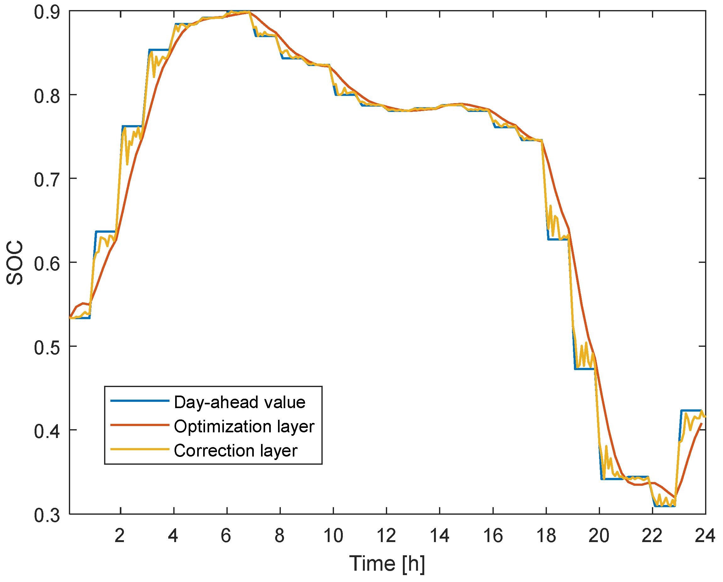
5.2.3. Comparative Analysis of Control Effect

To empirically verify the enhanced operational efficiency of the developed microgrid scheduling framework, a comparison was made between the optimization layer’s tracking of planned values and the correction layer’s tracking of interconnection power from the optimization layer, both with and without optimization. In addition, a comparison was made between the tracking of planned values in the optimization layer and the tracking of storage charging/discharging power states in the correction layer. Figure 9 illustrates the comparison of interconnection power tracking with the large grid, while Figure 10 presents the comparison of SOC tracking.

Figure 9 demonstrates that omitting hierarchical day-ahead optimization leads to marked fluctuations in microgrid interconnection power. These oscillations destabilize grid equilibrium, resulting in suboptimal scheduling controllability. However, by introducing hierarchical scheduling optimization, the fluctuations in interconnection power have been significantly smoothed, allowing it to align closely with the day-ahead planned values. This indicates that hierarchical scheduling optimization can effectively reduce the deviation between actual power output and predicted values, thus improving the controllability and stability of the system. Furthermore, the computational efficiency of hierarchical scheduling optimization is also very high, with a single optimization computation taking only about 0.4 s, which is sufficient to meet online application requirements. This demonstrates that the proposed coordinated optimization scheduling scheme is effective, achieving smooth and controllable scheduling of the microgrid’s connection to the distribution network while ensuring computational efficiency and system stability.

6. Conclusions

An improved dung beetle algorithm-based hierarchical strategy is introduced to address microgrid scheduling challenges. The conclusions derived from theoretical and simulation analyses are summarized as follows:

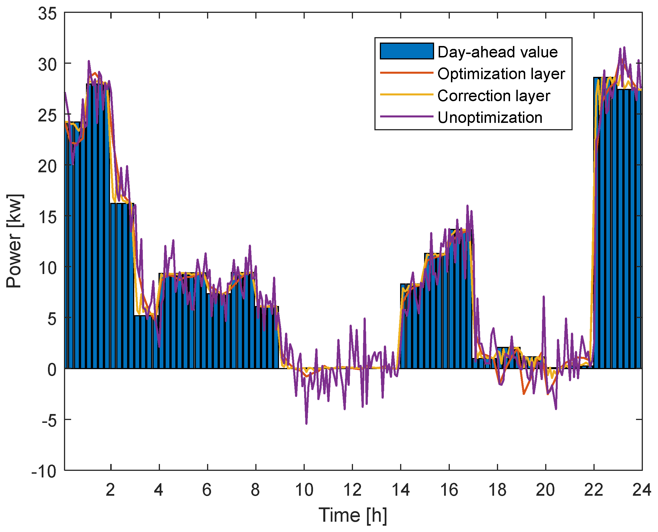
• The proposed three-layer predictive control model effectively improves the scheduling performance of the microgrid, stabilizing and controlling interconnection line power. It also considers time-varying electricity prices and environmental pollution costs, contributing to economic efficiency and sustainable development.
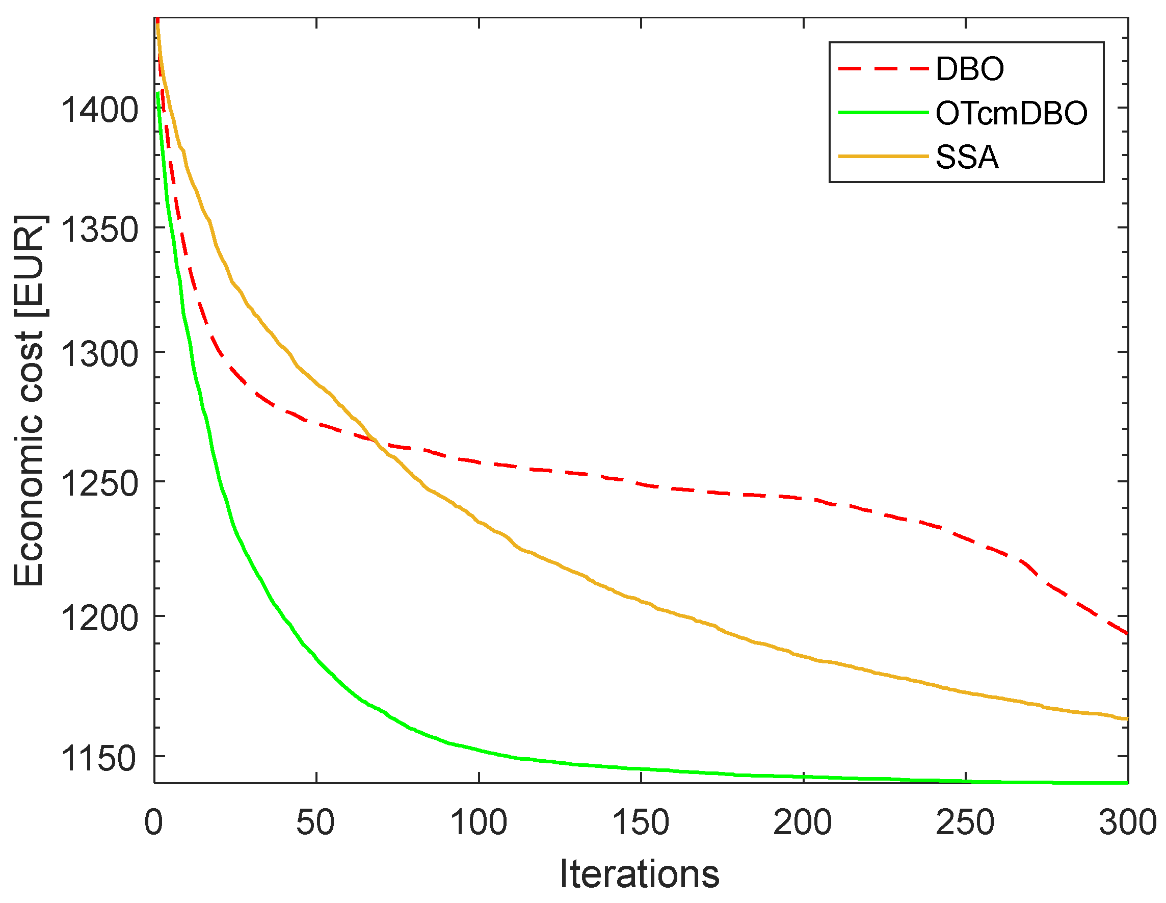
• Improvements to the traditional dung beetle optimizer algorithm, including population initialization, rolling behavior, and foraging behavior, along with mutation perturbations for the optimal solution, were compared through simulation experiments with other optimization algorithms. The results indicate that the OTcmDBO algorithm yields superior optimization results and converges more rapidly.
• The results of this study confirm the applicability of the proposed three-layer predictive control model and OTcmDBO algorithm to addressing renewable energy and load demand uncertainties in microgrids. While the findings demonstrate reductions in operating costs and improvements in volatility management, it is important to acknowledge limitations in the study. These include: (a) simplified assumptions in modeling (e.g., static energy storage parameters and deterministic load profiles); (b) dependence on day-ahead forecasting accuracy, which may degrade under extreme weather conditions; and (c) limited scalability for multi-microgrid collaborative scenarios.

Future research will focus on the following directions. (a) Expanding model adaptability: Validate the framework under more realistic conditions, including dynamic energy storage degradation models, probabilistic load forecasting, and multi-energy coupling scenarios. (b) Algorithm hybridization: Explore the integration of OTcmDBO with deep reinforcement learning to enhance real-time decision-making capabilities in high-dimensional uncertainty environments. (c) Cross-microgrid coordination: Extend the framework to interconnected microgrid clusters for regional energy sharing and ancillary service provision.

References

1. Chu, C.-C.; Wu, Y.-K.; Lian, K.-L.; Liu, J.-H. Guest Editorial Towards Resilient Power Grids Integrated With High-Penetrated Renewable Energy Sources: Challenges, Opportunities, Implementation Strategies, and Future Perspectives. IEEE Trans. Ind. Applicat. 2024, 60, 1960–1962. [Google Scholar] [CrossRef]
2. Rhodes, E.; Scott, W.A.; Jaccard, M. Designing flexible regulations to mitigate climate change: A cross-country comparative policy analysis. Energy Policy 2021, 156, 112419. [Google Scholar] [CrossRef]
3. Hu, J.; Shan, Y.; Yang, Y.; Parisio, A.; Li, Y.; Amjady, N.; Islam, S.; Cheng, K.W.; Guerrero, J.M.; Rodríguez, J. Economic Model Predictive Control for Microgrid Optimization: A Review. IEEE Trans. Smart Grid 2024, 15, 472–484. [Google Scholar] [CrossRef]
4. Babayomi, O.; Zhang, Z.; Dragicevic, T.; Hu, J.; Rodriguez, J. Smart grid evolution: Predictive control of distributed energy resources—A review. Int. J. Electr. Power Energy Syst. 2023, 147, 108812. [Google Scholar] [CrossRef]
5. Zhang, Q.; Chen, X.; Li, G.; Feng, J.; Yang, A. Model Predictive Control Method of Multi-Energy Flow System Considering Wind Power Consumption. IEEE Access 2023, 11, 86697–86710. [Google Scholar] [CrossRef]
6. Hu, Z.; Liu, S.; Luo, W.; Wu, L. Intrusion-Detector-Dependent Distributed Economic Model Predictive Control for Load Frequency Regulation With PEVs Under Cyber Attacks. IEEE Trans. Circuits Syst. I 2021, 68, 3857–3868. [Google Scholar] [CrossRef]
7. Wang, Y.; Liu, C.; Liu, Z.; Wang, T.; Ke, F.; Yang, D.; Zhang, D.; Miao, S. A Hierarchical Cooperative Frequency Regulation Control Strategy of Wind-Storage-Load in a Microgrid Based on Model Prediction. Energies 2023, 16, 1886. [Google Scholar] [CrossRef]
8. He, Y.; Li, Z.; Zhang, J.; Shi, G.; Cao, W. Day-ahead and intraday multi-time scale microgrid scheduling based on light robustness and MPC. Int. J. Electr. Power Energy Syst. 2023, 144, 108546. [Google Scholar] [CrossRef]
9. Zhang, J.; Qin, D.; Ye, Y.; He, Y.; Fu, X.; Yang, J.; Shi, G.; Zhang, H. Multi-Time Scale Economic Scheduling Method Based on Day-Ahead Robust Optimization and Intraday MPC Rolling Optimization for Microgrid. IEEE Access 2021, 9, 140315–140324. [Google Scholar] [CrossRef]
10. Hou, J.; Yu, W.; Xu, Z.; Ge, Q.; Li, Z.; Meng, Y. Multi-time scale optimization scheduling of microgrid considering source and load uncertainty. Electr. Power Syst. Res. 2023, 216, 109037. [Google Scholar] [CrossRef]
11. Zhang, N.; Ren, Q.; Liu, G.; Guo, L.; Li, J. Short-term PV Output Power Forecasting Based on CEEMDAN-AE-GRU. J. Electr. Eng. Technol. 2022, 17, 1183–1194. [Google Scholar] [CrossRef]
12. Fu, S.; Sun, H.; Liu, Z.; Han, H.; Zhang, Y. Model Predictive Control for Nonlinear Systems With Two-Time Scales. IEEE Trans. Automat. Sci. Eng. 2024, 21, 5088–5098. [Google Scholar] [CrossRef]
13. Lin, Y.; Wending, C.; Zhuo, L. Hierarchical Prediction Control Strategy of Active Power for Photovoltaic Cluster. Dianli Xitong Zidonghua/Autom. Electr. Power Syst. 2023, 47, 42–52. [Google Scholar] [CrossRef]
14. Hu, K.; Wang, B.; Cao, S.; Li, W.; Wang, L. A novel model predictive control strategy for multi-time scale optimal scheduling of integrated energy system. Energy Rep. 2022, 8, 7420–7433. [Google Scholar] [CrossRef]
15. Dey, B.; Misra, S.; Marquez, F.P.G. Microgrid system energy management with demand response program for clean and economical operation. Appl. Energy 2023, 334, 120717. [Google Scholar] [CrossRef]
16. Xue, J.; Shen, B. Dung beetle optimizer: A new meta-heuristic algorithm for global optimization. J. Supercomput. 2023, 79, 7305–7336. [Google Scholar] [CrossRef]
17. Dehghani, M.; Trojovský, P. Osprey optimization algorithm: A new bio-inspired metaheuristic algorithm for solving engineering optimization problems. Front. Mech. Eng. 2023, 8, 1126450. [Google Scholar] [CrossRef]
18. Gao, Z.-M.; Zhao, J.; Zhang, Y.-J. Review of chaotic mapping enabled nature-inspired algorithms. Math. Biosci. Eng. 2022, 19, 8215–8258. [Google Scholar] [CrossRef]
19. Aryani, D.R.; Song, H. A Review on Power System Security Issues in the High Renewable Energy Penetration Environment. J. Electr. Eng. Technol. 2024, 19, 4649–4665. [Google Scholar] [CrossRef]
20. Zhang, H.; Huang, Q.; Ma, L.; Zhang, Z. Sparrow search algorithm with adaptive t distribution for multi-objective low-carbon multimodal transportation planning problem with fuzzy demand and fuzzy time. Expert Syst. Appl. 2024, 238, 122042. [Google Scholar] [CrossRef]
21. Zhang, Y.; Liu, L.; He, D. Application of Variable Universe Fuzzy PID Controller Based on ISSA in Bridge Crane Control. Electronics 2024, 13, 3534. [Google Scholar] [CrossRef]
22. Ou, X.; Wu, M.; Pu, Y.; Tu, B.; Zhang, G.; Xu, Z. Cuckoo search algorithm with fuzzy logic and Gauss–Cauchy for minimizing localization error of WSN. Appl. Soft Comput. 2022, 125, 109211. [Google Scholar] [CrossRef]
23. Zhang, J.; Zhang, Q.; Li, G.; Wu, J.; Wang, C.; Li, Z. Hybrid Model for Renewable Energy and Load Forecasting Based on Data Mining and EWT. J. Electr. Eng. Technol. 2022, 17, 1517–1532. [Google Scholar] [CrossRef]
Figure 2. Intraday real-time scheduling process.
Electronics 14 01829 g002
Figure 3. The convergence curve of the test function.
Electronics 14 01829 g003
Figure 5. Wind power, PV, and load power forecast.
Electronics 14 01829 g005
Figure 6. Economic convergence curves of the three algorithms.
Electronics 14 01829 g006
Figure 7. Output of each unit at optimal economic cost.
Electronics 14 01829 g007
Figure 8. The output of each unit in the optimized layer.
Electronics 14 01829 g008
Figure 9. Optimized layer contact line power tracking.
Electronics 14 01829 g009
Figure 10. Optimized layer energy storage SOC tracking.
Electronics 14 01829 g010