Abstract
The constant rise of malicious URLs continues to pose significant threats and challenges in cybersecurity, with attackers increasingly evading classical detection methods like blacklists and heuristic-based systems. While machine learning (ML) techniques such as SVMs and CNNs have improved detection, their accuracy and scalability remain limited for emerging adversarial approaches. Quantum machine learning (QML) is a transformative strategy that relies on quantum computation and high-dimensional feature spaces to potentially overcome classical computational limitations. However, the accuracy of QML models such as QSVM and QCNN for URL detection in comparison to classical models remains unexplored. This study evaluates ML models (SVMs and CNNs) and QML models (QSVMs and QCNNs) on a dataset, employing data preprocessing techniques such as outliers, feature scaling and feature selection with ANOVA and PCA. Quantum models utilized ZZFeatureMap and ZFeatureMap for data encoding, to transfer original data to qubits. The achieved results showed that CNNs outperformed QCNNs and QSVMs outperformed SVMs in the performance evaluation, demonstrating a competitive potential of quantum computing. QML shows promise for cybersecurity, particularly given the QSVM’s kernel advantages, but current hardware limits the QCNN’s practicality. The significance of this research is to contribute to the growing body of knowledge in cybersecurity by providing a comparative analysis of classical and quantum ML models for classifying malicious URLs.
1. Introduction
The development of novel technologies for communication has played a major role in the growing popularity and marketing of organizations in a variety of industries such as finance, retail, health and education. Actually, maintaining a presence on the internet at present is almost a necessity to run a profitable organization, resulting in a constant rise in the significance of the web. However, increasingly advanced methods for attacking and defrauding users have been made possible by technical improvements. Attacks of this type include deceiving individuals into disclosing personal information that could potentially be utilized in stealing money and identities as well as installing malware on a user’s device. These attacks mentioned may be carried out through a broad range of methods like ransomwares, spywares, watering holes, phishing and several more. It is challenging to develop reliable approaches to identify cybersecurity breaches due to the wide range of attacks and the possibilities of newly created attack types. Given the exponential rise in these newly formed security threats, the rapid growth of new technologies and the limited availability of security professionals, the drawbacks of traditional security management become progressively problematic. The dissemination of hacked URLs is a major component of “most attack” strategies or can be the means by which those attacks are carried out [1]. A uniform resource locator or URL (Figure 1) is the worldwide address of files and “other resources on the World Wide Web (www)”, as defined by many research and media outlets. There are two primary parts that comprise a URL; the first part is the protocol identifier, and the second part is the resource name that indicates the domain name and IP address of the resource.
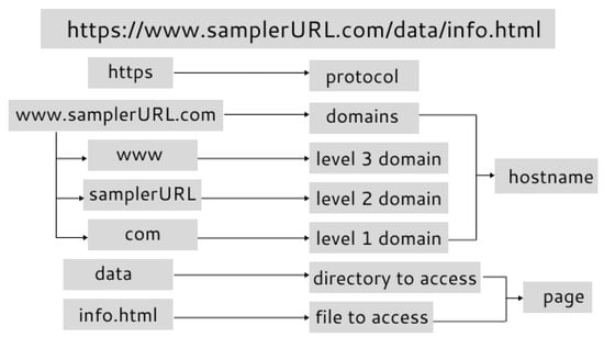
Figure 1.
Structure of the URL.
A malicious URL is a compromised URL because such web addresses are designed to cause harm to a device and its users. Actually, Ref. [2] mentioned “that close to one third of all websites are potentially malicious in nature” which illustrates the common use of malicious URLs in cybercrimes. Malicious URLs can lead to various types of cyber threats including malware, phishing, defacement and other malicious activities, as mentioned before. In malware, users are typically taken to a malicious website through fraudulent URLs where malware may be installed on the device, leading to identity theft, keystroke recording and even corrupting files on the device. Additional examples include computer worms and viruses, ransomware, spyware, keyloggers and the common drive-by downloads that trick users into visiting a malicious website and unintentionally downloading the malware. Ref. [3] reported that “malware continued to lead the Attack Techniques chart with 35.9 percent up from 34.7 percent” in the “2024 Cyber Attacks Statistics”. Meanwhile, in phishing, malicious URLs can be made to appear authentic by utilizing obfuscation methods such as URL shortening or misspelled domain names, for example, “www.g00gle.com” rather than “www.google.com”. In light of this, researchers suggested approaches that may be applied to eradicate or, at the very least, minimize the impacts of such threats brought on by malicious URLs. Traditional detection techniques including blacklisting and heuristic-based approaches were the first to solve such issues until threat actors discovered new ways to evade the system. While several researchers began making tremendous use of cutting-edge approaches given by machine learning (ML), attackers are still employing sophisticated methods to still evade the system. Researchers are now studying quantum computing (QC), a new technology that is still in its earliest stages but has the potential to be extremely powerful and transformative by leveraging quantum computing’s unique characteristics, superposition and entanglement to potentially overcome these limitations. Quantum kernels and quantum circuit models such as QSVMs and QCNNs offer computational advantages by fundamentally changing data processing. The QSVM leverages quantum kernel methods, such as the ZZFeatureMap, to project classical data into high-dimensional quantum feature spaces, enabling the efficient separation of complex patterns that challenge classical SVMs. Similarly, QCNNs apply quantum circuits to extract hierarchical features, though their adaptation to classical data remains constrained by current hardware. Quantum computers can be employed to minimize the time needed for machine learning training and enhance AI’s skills in tackling difficult real-world challenges [4]. Empirical studies highlight QML’s growing role in cybersecurity. The study in [5] showed a 40 percent faster training time using the QSVM for intrusion detection on simulators while achieving a 99 percent accuracy in phishing URL detection using hybrid quantum classical models [6]. However, these advances are tampered with limitations such as a limited number of qubits, as quantum systems require a sufficient amount to handle complex computations. Coherence times used to mark the duration for which qubits maintain a quantum state are often too short for lengthy computations. Additionally, high error rates in quantum operations demand effective error correction methods, which are still in development [4].
To conclude, this research seeks to explore the potential advantages of quantum machine learning in cybersecurity by evaluating its effectiveness in malicious URL classification. By comparing classical ML models (SVMs and CNNs) with their quantum counterparts (QSVMs and QCNNs), this study aims to assess whether quantum computing can provide tangible improvements in accuracy, efficiency and resilience over conventional techniques. The findings of this research will contribute to the ongoing discourse on the applicability of quantum-enhanced models in real-world cybersecurity challenges, providing insights into their viability for threat detection and mitigation.
2. Literature Review
The daily lives of humans are now completely dependent on the internet, but as its use continues to advance, so does the risk of cyberattacks. Malicious URLs, essentially, are one of the primary methods that cybercriminals use to distribute cyberattacks (malware and phishing scams) and compromise user security. In an effort to combat this, researchers continue to investigate the effectiveness of machine learning and explore the potential possibilities of quantum machine learning as quantum computing emerges. This chapter fulfills the first research objective stated in Section 1. The first two types of methods for identifying fraudulent URLs include rules-based and machine learning-based techniques, until the exploration of quantum-based techniques to support classical machine learning models. Figure 2 depicts the taxanomy used to classify reviewed papers. It presents a extensive overview of the explored studies based on the detection of malicious URLs according to rule-based, ML/DL and QML-based techniques.
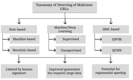
Figure 2.
Taxonomy of malicious URL detection techniques.
2.1. Rules-Based/Traditional Detection Techniques
A variety of approaches for identifying and preventing fraudulent websites and URLs have been developed in order to protect the privacy and security of internet users. Traditionally and popularly, the two approaches developed are the blacklist-based approach and heuristic-based approach.
2.1.1. Blacklist-Based Approach
“A blacklist contains a list of suspicious domains, URLs and IP addresses, which are used to validate if a URL is fraudulent” [7], bringing about the approach of maintaining a database of URLs that have been identified as malicious. Over time, this database is compiled, usually, through “crowd-sourcing solutions like PhishTank” if it is discovered that a certain URL is fraudulent, and cybersecurity firms also take part in curating this database. In regard to how the blacklist approach works, any URL a user is attempting to access is checked against the existing blacklist in the database and access to the URL is prohibited if it is found in the database, alerting the user of the possible threats associated with the URL. Anti-malware and phishing toolbars that are publicly available, such as Google Safe Browsing, employ the blacklist approach extensively [7] because these toolbars keep a list of URLs that are deemed malicious and alert users upon stumbling across on discussed URLs.
Limitations of the Blacklist-Based Approach
A method of blacklisting was proposed by [8] called “PhishNet” for predicting phishing URLs by utilizing the “directory structure, comparable IP addresses and brand name” to identify malicious URLs from current blacklisted URLs. Additionally, Ref. [9] created an approach as part of the categorization process and “compared the domain name and name server” data of newly discovered suspicious URLs to the data of URLs that have been blacklisted. However, there are limitations to blacklist approaches. Considering how thousands of fraudulent websites are created daily, the list is in continual need of an update to reflect the evolving landscape of malicious URLs; [10] consequently demonstrated this theory using fabricated domains where these domains were attached to the blacklist and, after a significant amount of time, around “50–80” percent of the fabricated domains were added after the attack had been executed. In relation to the difficulty of maintaining an exhaustive list, the blacklist-based approach was anticipated to have low false positive rates by several researchers, hence failing against newly generated URLs. Another limitation to the blacklist-based approach involves threat actors employing new IP addresses, subdomains or domains to avoid detection. Hence, Ref. [11] established that there are four different methods of obfuscation, including “Obfuscating the Host with an IP, Obfuscating the Host with another domain, Obfuscating the host with large host names and misspelling”, as all of these methods attempt to conceal the malicious URL in order to camouflage the website’s nefarious intentions. After the URL seems authentic, users access it, and the attack can commence. There is a malicious code inserted into the “JavaScript” that enables this attack to be executed and attackers frequently attempt to conceal the code in order to evade detection by signature-based tools. Threat actors employ a variety of alternative techniques in evading blacklists, including “fast flux that utilizes algorithm creation to develop proxies automatically to host web pages” [12].
2.1.2. Heuristic-Based Approach
A “blacklist of signatures” [13] is completely based on signatures that are employed to establish a link between “the signature of an existing malicious URL” and the newly created URL. The heuristic-based approach is an expansion of the blacklist-based approach, which detects fraudulent websites using a variety of methods including “behavior-based, content-based and signature-based” techniques. This approach entails analyzing the various characteristics and features contained in a URL or web content to identify if it displays any patterns commonly associated with malicious activities; hence, it is proven to possess better “generalization capabilities” as compared to the blacklist-based approach as it may identify and recognize newly generated URLs created to cause cyber harm faster.
- Signature-based Technique: It relies entirely on malicious patterns and signatures of a URL contained in a database. These signatures are derived from the URLs itself, the web content it is pointed to or the payloads delivered by fraudulent websites.
- Behavior-based Technique: The runtime behavior of webpages or applications linked to a URL are monitored and analyzed utilizing behavior-based techniques. This technique involves observing the actions taken by the web content such as file modifications, network traffic patterns, interactions and system calls with several other processes or services.
- Content-based Technique: This technique searches for and identifies potentially harmful activity by analyzing the content of the files or web pages that are associated to a URL.
Limitations of the Heuristic-Based Approach
A heuristic-based approach may instantly detect newly generated fraudulent websites in real-time. However, this approach has its limitations since attackers frequently use pattern shifts and obfuscation tactics to avoid recognizing signatures; hence, it neglects specific attempts that lead to “zero-day exploits” [14]. This approach has a similar drawback to the blacklist-based approach since it can be worked around by utilizing an obfuscation method, including creating a massive number of URLs using an algorithm that can evade both the blacklist and heuristic techniques as both cannot handle large lists due to rapidly changing technologies. Consequently, Ref. [15] mentioned that these techniques were developed especially for a small set of common threats and are not applicable to all varieties of emerging fraudulent websites.
2.2. Machine Learning for Malicious URL Detection
Researchers across a variety of fields such as healthcare, security, banking, privacy, agriculture, insurance, weather forecasting, stock market and several other fields have particularly been interested in machine learning. Cybersecurity researchers over a decade have been utilizing machine learning algorithms and methods for malicious URL detection to overcome the limitations of traditional-based detections. Machine learning methods can effectively learn from vast amounts of data, which enables a faster identification of fraudulent websites that were previously undiscovered. In addition, these methods encompass the ability to learn from past experiences, where self-learning is enabled without requiring human interaction [16]. To overcome the limitations of using rules-based approaches, the global research communities across the world have used a variety of effective ML techniques to address these issues and have made substantial progress in identifying malicious URLs. In regard to detecting malicious URLs, supervised, unsupervised and deep learning are key ML techniques as each of these methods has distinct approaches in identifying such URLs.
2.2.1. Supervised Learning (SL)
SL is the most commonly used CML approach to detecting malicious URLs. It is a kind of ML in which an algorithm can learn from labelled data, where the algorithm is fed with a dataset containing both input and output with, in this case, “benign” and “malicious” labels with a goal to learn and understand the relationships between inputs and outputs so that it can make predictions on new and unseen data. For an ML model to be successful, it is dependent on the quality of training data utilized, as this crucially determines the performance output of the model; hence, it can lead to feature representation, where [13] mentioned the “process” of representing features as two phases that include feature collection and feature preprocessing. This section will discuss the feature representation and the two commonly used SL algorithms, sector vector machines (SVMs) and logistic regression (LR).
Feature Collection
The goal of this step is engineering focused, aiming to gather important information on the URL. This important information is described as features that are obtained from a blacklist of URLs. These features are as follows:
- Lexical Features: “Lexical Features are collected through lexical scanning” [17] derived from the layout and structure of the URL string or name itself, without gaining access to the content of the website or requiring network analysis to be conducted. In summary, it comprises the characteristics of the URL string such as length, hyphens, special characters, number of dots and suspicious keywords present including “update” and “login”. Ref. [13], mentioned that the use of lexical features as a first line of defense in detecting malicious URLs is important due to the possession of a low computational state and reasonable effectiveness.
- Content Features: The content features are extracted directly from the actual web page or a resource that the URL is connected to and can be obtained when the website is visited or downloaded. These webpage contents include HTML and JavaScript codes, embedded links, the presence of iframes, etc. Content features are classified as “heavy weight” due to the requirement of excess information to be extracted, which, in turn, may raise security issues [13]. Although collecting and analyzing the online content is necessary for these features, it can be computationally demanding and frequently yields to a deeper understanding of the page’s nature.
- Network/Host-based Features: “Network features are a union of the domain name system (DNS), network and host features” [17] and these features often require active probing or monitoring of network traffic. These features include WHOIS and DNS information, IP address properties, server location, etc. Ref. [17] further discussed how research has often shown that “legitimate websites” possess additional contents compared to fraudulent sites, and network features can be beneficial in identifying fraudulent sites, which are frequently “hosted by less” reliable “service providers”. Furthermore, these fraudulent websites can be identified using information derived from the DNS, which may be compared with a list of frequently utilized keywords linked to malicious actions.
Feature Preprocessing
This step feeds ML algorithms with raw data on URLs such as “textural description” by means of formatting the data approximately and converting it to a numerical vector. The numerical data can be utilized just as is and textual and lexical contents can be represented using “bag-of words”. The bag-of-words model has been successful in the identification of malicious URLs as “it is a natural extension of applying NLP-based deep learning (DL) models” to the issue [18]; hence, these models are able to draw out the features from unstructured text input for feature extraction. This issue is solved by the convolutional neural network (CNN) algorithm, which will be discussed later.
Support Vector Machine
The SVM is a commonly used SL model for classification or regression. It performs especially well for binary classification problems, which, in this study, means distinguishing between malicious and benign URLs, because it is effective in determining the most suitable border between data points belonging to distinct classes. The main idea behind SVMs is to determine the optimal hyperplane that separates data into different classes with the maximum margin, specifically, the gap between the hyperplane and the closest data points of the distinct classes. The data are efficiently divided into several classes using this hyperplane. In a two-dimensional and three-dimensional space, a hyperplane is a line and plane, respectively, but it becomes a hyperplane in a higher dimension. The SVM is a type of linear classifier, although it can be extended to solve non-linear classification problems. In [6], researchers utilized three different kernels for the SVM model, namely, Sigmoid, RBF and Poly, because the primary principle of these kernels is employed for handling linearly indivisible data by combining the original features in non-linear ways and projecting them onto higher-dimensional space by means of a mapping function ⌀, which, in turn, renders the data “linearly separable”. These kernels were denoted as follows:
- Sigmoid:
- Polynomial of degree k:
- Radial Basis Function (RBF) or Gaussian Kernel:
The SVM with RBF resulted as the second best and Poly kernel the third best after one of the three neural networks also utilized in the study resulted in being the best in analyzing the dataset. However, SVMs have many strengths, but they also have some very noticeable challenges. A research study of SVMs conducted by [19] mentioned that these weaknesses include “algorithmic complexity”, which impacts how long how long it takes a classifier to train on large data sets, developing the best classifiers for multi-classification issues and the “performance of SVMs in imbalanced datasets”.
Logistic Regression
LR [6] is another commonly utilized discriminative model, defined as a “statistical technique” used in modeling the connection between “independent variables and a categorical, usually binary dependent variable”. LR, as an approach, operates by estimating the likelihood that an observation falls into a specific category or group. Depending on the independent variables, it predicts the likelihood that a binary-based variable will have a value of 1 or 0 and does this by utilizing a logistic function. The logistic function converts the result obtained from LR to a number between 0 and 1, which can be utilized to represent the likelihood of falling into a particular category. The logistic function is given as follows:
Authors [20] concentrated on applying LR to detect fraudulent URLs through feature extraction, hence utilizing LR to differentiate benign and malicious URLs, although researchers also utilized several other models such as SVMs, K-nearest neighbors (KNN) and linear discriminant analysis (LDA) to compare and evaluate performance metrics of each model on dataset. Ref. [21] proposed a novelty anti-phishing framework that focuses on the extraction of client-side features exclusively. The approach provides a method that utilizes information discovered in hyperlinks in the website’s source code for the identification of phishing websites. The proposed framework using LR performed the best out of all the algorithms used and, when compared and evaluated with other approaches, gave the best results. Ref. [22] discussed the challenges of using LR, saying that choosing the appropriate variables to include in the LR model is essential for it to be successful. Although it may be tempting to incorporate as many input variables as possible, doing that might reveal misleading associations or dilute “true associations”, which can result in huge standard errors with inaccurate “confidence intervals”.
2.2.2. Unsupervised Learning (UL)
UL occurs when the real label of data is unavailable during the training phase of models. UL methods characterize an anomaly as unusual behavior that, hence, depends on anomaly detection. These algorithms are “clustering and 1-class SVMs” that are applied to anomaly identification in the literature. Unfortunately, it might be challenging to distinguish between “normal behavior” and anomalies, as URLs are “extremely diverse”. Consequently, these methods have not gained much popularity in detecting malicious URLs; however, to increase the performance of studies, various approaches have attempted to combine both SL and UL methods together. For instance, Ref. [23] introduces an “anomaly detection framework for phishing URL detection based on a convolutional autoencoder (CAE)”. Researchers, utilizing only benign URLs, trained the autoencoders to create a URL template and used the properties of the autoencoder to lower “reconstruction performance for unobserved” data, establishing the anomalous score of phishing. The framework went through a comprehensive test on “three real-world datasets” containing “222,541 URLs” and produced the best results, although the framework was limited to exclusively optimizing the characteristics of “character-level features” among the several characteristics that make up URLs.
2.2.3. Deep Learning (DL)
With significant advances in computer vision and natural language processing (NLP), DL has emerged to solve problems in data mining and ML. Specifically, DL is aimed to extract relevant characteristics directly from unstructured or raw input and use these characteristics for classification, which can, in turn, lessen the need for rigorous feature engineering for malicious URL detection and enable the construction of models without domain knowledge. The convolutional neural network (CNN) extracts information from input images by applying mathematical convolutional operators, making it the most popular amongst most deep learning models for image categorization. Although CNNs are traditionally used for image data, they can be adapted to text-based analysis using NLP. As mentioned earlier, bag-of-words have been effective in the detection of malicious URLs; hence, the possibilities of using NLP-based models to detect malicious URLs is made acceptable due to their capacity to extract features from an unstructured text input. For instance, a study called “eXpose”, conducted by [24], used character-level convolutional networks in the application of URL string in an attempt to identify patterns of certain characters in occurrence together. Dissimilar to the earlier methods that mostly depended on bag-of-words, the researcher’s approach failed to observe the crash in the number of characteristics since word encoding was not employed. Despite the failed observation, the approach performed better than that using SVMs on bag-of-words. Another novel approach named “URLNet”, proposed by [25], created a framework to detect malicious URLs, applying convolutions in capturing both the words and characters and several types of information obtained from URLs. By combining character-level and word-level information, there was a significant improvement in the performance of the system. Although the research is innovative, yielding impressive outcomes, its effectiveness in a real-word deployment is yet to be confirmed, as implementing such deep learning methods may hinder some applications.
Challenges with ML Algorithms
Despite that ML algorithms for detecting malicious URLs have made significant progress, their efficiency is hindered by a number of issues not limited to the following:
- High volume and velocity: On the internet, there is a staggering number of URLs created daily, making “real-world URL” a type of large data (big data) that has “high velocity and volume”. In [26], an estimation indicated that 175 new websites are generated every minute, thus creating about 252,000 new websites everyday throughout the world. This big data of URLs necessitates scalable ML solutions capable of analyzing and processing such vast amounts of data in real-time, which traditional ML algorithms may find difficult and computationally exhausting.
- Difficulty in obtaining labels: As discussed earlier, SL algorithms comprise the majority of ML methods utilized in detecting malicious URLs, in which a requirement for labelled data (malicious and benign) to train on is necessary. Labelling URLs as malicious or benign requires either human expertise to label the data or obtaining it through blacklists and whitelists (where data also go through manual labelling). Unfortunately, as compared to the total amount of accessible URLs on the internet, labelled data are in limited amounts and often unavailable. However, there have been strategies to resolve this issue, aiming to maximize the value of limited labelled data, including exploring active learning and semi-supervised learning.
- Concept Drift and Adversarial attacks: In malicious URL detection, techniques and strategies used by threat actors evolve overtime as ML models become efficient in detecting such URLs. The emergence of new threats and supplicated approaches creates a moving target problem for ML models, as it frequently requires the models to be updated and retrained to cope with new threats, which can be computationally overwhelming.
2.3. Quantum Machine Learning for Detecting Malicious URLs
Compared to classical computing, QC processes information in completely different ways by utilizing the ideas of quantum physics. Quantum bits, also called qubits for short, are the fundamental units of QC where, due to superposition, they can simultaneously represent 0 and 1 and can be entangled to work together in complex ways. The main goal of QC is to provide solutions to problems that classical computing cannot solve [27]. In [6], “the state of a qubit over the computational basis , is defined as follows:
where , and , are referred to as state amplitudes, allowing QCs to perform huge calculations simultaneously.
A collection of qubits called registers are used to store and manage quantum information, given as . Qubits are manipulated by quantum gates through unitary transformation of changing the state of qubits, taking advantage of superposition as well as entanglement and the fundamental components of quantum circuits, which are similar to classical logic gates.
2.3.1. Quantum Machine Learning
To improve computing capability and efficiency, QML combines quantum algorithms with classical ML methods. There are improvements in the development of quantum versions of classical algorithms such as QSVMs and QCNNs, which have been studied by researchers and show potential in speeding up certain tasks.
Quantum Sector Vector Machine
The QSVM (Figure 3) is a quantum equivalent to the classical SVM and, when compared, could potentially handle classification problems more quickly or effectively by utilizing the concepts of QC. The main idea of QSVMs is to utilize “quantum algorithms” for both “quantum kernel estimation and linear systems” to map data into high-dimensional quantum space, where data are easier to separate using the quantum hyperplane within the process of utilizing QCs [5,28]. When performing a QSVM classification, the best hyperplane is identified and then represented by “vector w” within the data space. That vector divides the matrix space into two classes that are required. These classes are denoted as follows:
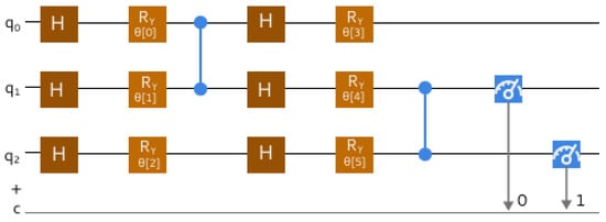
Figure 3.
The QSVM circuit model. Adapted from [5].
mapping to class +1, mapping to class −1, and with hyperplane displacement being denoted as .
Conventional linear algebra algorithms require steps to calculate parameters w and b, which describe the hyperplane given an accuracy of . Additionally, determining the hyperplane that separates, in this instance, falls to reducing the norm while retaining the awareness of . Furthermore, it is straightforward to employ the sample used to train the “correlation matrix of vectors” to construct a separation of hyperplanes.
Quantum Convolutional Neural Network
The initial quantum neural computing network (Figure 4) was proposed by [29], where the author demonstrated how to substitute quantum states with phases and amplitudes for conventional signals entering the neurons and at the neuron’s output; a quantum is likewise created, which is dependent on “the linear superposition” of the input states.
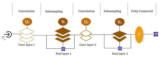
Figure 4.
The QCNN circuit model. Adapted from [5].
For a given dimension, a convolutional layer employs “a single quasi-local unitary in a translationally invariant” way [5]. Consequently, a portion of qubits are examined for sub-sampling, where the results obtained dictate the “unitary rotation ” applied to adjacent qubits, therefore lowering the degree of freedom that leads to non-linearities in QCNN. This process is continuous until the system size is small enough where, with qubits remainders, an entire layer is used as a unitary F. A QCNN for the classification of “N-qubit input state” is represented as parameters and all unitary are initialized during training and gradual optimization until convergence.
2.3.2. Potential of QML in Detecting Malicious URLs
Although vast amounts of data are computed using ML algorithms, quantum-enhanced ML takes advantage of the quantum system for the improvement of computational speed and enhancement of data processing performed by the algorithms. QC technology is one of the emerging techniques that holds potential in ML since it can analyze large datasets instantly and solve optimization problems [30]. Ref. [6] examined the potential use of QML to detect malicious URLs in an effort to increase the tools available to counter phishing threats and compared the findings with those of the classical ML approaches. Their proposed model was developed on the basis of “Deming Cycle or PDCA (Plan, Do, Check, Act)”, where the phases of the research study were done iteratively for both CML and QML. The researchers used a labelled dataset containing all three features (network, content and lexical) and analyzed the dataset with ML models such as LR, DT, SVM and NN. The authors moved on to the QML proposed model, named “SVM/Q-VQC”, where they used the variational quantum classifier (VQC) for training, in which “data coding features (such as ZZFeatureMap, ZFeatureMap and PauliFeatureMap), Ansatz, also known as quantum circuits (such as RealAmplitudes, EfficientSU2 and ExcitationingPreserving), and optimization algorithms (COBYLA (Constrained Optimization By Linear Approximation), GradientDescent (Gradient Descent minimization routine) and SLSQP (Sequential Least Square Programming optimizer))” were iteratively combined to achieve the best results of the classifier, after which both CML and QML results were evaluated and compared.
The primary goal in [27] was to present the idea of QC in the context of detecting malware by evaluating the accuracy of both quantum and classical convolutional models to detect malware in the Android environment, making it “the first attempt to introduce quantum computing in image-based malware detection” so far. The researchers achieved this by collecting a dataset of Android applications that have gone through conversion (converting applications to grayscale images) and using a set of convolutional and quantum models to develop a classifier with the aim of differentiating between malware and trusted applications by taking into consideration Grad-CAM, “to provide explainability in terms of graphical information about the area of the images that influenced the prediction”.
Intrusion detection aimed at comparing basic QML models [5] such as the QSVM and QCNN in understanding their power while handling a large amount of data. Utilizing the same dataset and approach, researchers trained their respective CML models, SVM and CNN, evaluating and comparing the results at the end.
2.3.3. Challenges and Limitations of QML
The advantages of QML over CML have not yet been thoroughly and convincingly proven. Some hybrid QC experimental cases (Table 1) show promise for the “mid-term future”; however, currently, there are just a few particular instances in which some “quantum-inspired” methods have produced little incremental benefits [31]. Consequently, demonstrating the present and prospective benefits of QML techniques is challenging due to the high level of noise in QCs and the limited number of qubits for testing. Despite QML’s potentiality to speed up computations and improve accuracy, QML faces a common limitation in every research study conducted on it, which is a hardware limitation. QC is still in its early stage and the results are still very theoretical. Due to the present constraints on quantum hardware, its application in the realm of cybersecurity is particularly more limited. Classical ML outperformed QML models [6] because CML models have been thoroughly researched and optimized for years and there is an abundance of scholarly materials available on the subject, whilst QML is limited. Ref. [27] also experienced a similar limitation when the quantum models used for the experimentation could not use image dimensions “bigger than 25 × 1”. However, Ref. [5] was not limited due to hardware restrictions, as QML classifiers surpassed classical ML classifiers, showing superiority and a more reduced training time by about two times in the presence of huge datasets utilized in their related research study.

Table 1.
Comparison between CML and QML.
Software limitations can arise due to optimization techniques relying on variational methods, where parameters of quantum circuits are optimized using classical techniques. This can be computationally intensive and may require numerous iterations, especially for complex models specifically.
2.3.4. Gap in Research and Conclusion
Pertaining to the classification of malicious URLs, numerous classical machine learning (CML) models have been developed to enhance the detection process and improve performance rates. However, the exploration of quantum machine learning (QML) models in this domain remains limited due to the emerging nature of quantum computing (QC) and its constraints in hardware and software resources, making it challenging to refine QML models. Based on an extensive review of published research, it appears that [6] may be among the few, if not the only, researchers to have implemented QML for malicious URL classification, utilizing variational quantum classifiers (VQC).
Rather than proposing a novel detection approach, this research aims to expand the existing body of knowledge by conducting a comparative analysis of CML models and their QML counterparts—SVM vs. QSVM and CNN vs. QCNN—to evaluate their effectiveness in accurately identifying malicious URLs. This study not only assesses the feasibility of QML in cybersecurity but also explores its potential applicability across other research domains.
3. Methodology
A mixed approach (Figure 5) of both qualitative and quantitative approaches is taken into consideration. Combining both techniques provides a comprehensive analysis and understanding of the dataset, which is necessary to accomplish the aim of this research. The quality of data utilized crucially determines the performance output of CML and QML models or classifiers as the feature extraction and selection process enables models to train efficiently. The qualitative technique involved a systematic literature review conducted where relevant papers were analyzed, producing detailed information about the datasets, the classifiers used and the outcomes of these papers. The methodology of this research is structured according to testing and comparing CML and QML models for the detection of malicious URLs. This section outlines the approach for this study, focusing on both the theoretical and practical outcomes of the research direction. For a full understanding and assessment of models, both qualitative and quantitative methods are employed, taking into account the legal and ethical considerations addressed to ensure the integrity and societal impact of the research study. The research process is depicted in Figure 5, giving the overview of the research flowchart.
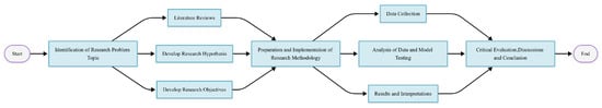
Figure 5.
Research Process for current study.
This study will use secondary data for the purpose of detecting malicious URLs. CQ (classical data with ML algorithms executing on quantum hardware) was used in this study to execute simulations on classical hardware, where classical data is encoded first by related quantum algorithms (see Figure 6). The experimental setup involves setting up the environment and necessary software tools as well as defining the parameters for model training. The experiments were conducted on an Ubuntu virtual machine hosted on a Windows 11 OS (Operating System) laptop in Google Colaboratory (Colab in short) that hosts an open-source project called Jupyter Notebook (https://colab.google/ (accessed on 23 April 2025)). This service offers free access to online computational resources such as GPUs (Graphical Processing Units) for enhancing the graphical performance of the computer and TPUs (Tensor Processing Units) to accelerate handling projects on both CML and QML models. For this experiment, the software libraries and dependencies utilized are as follows:
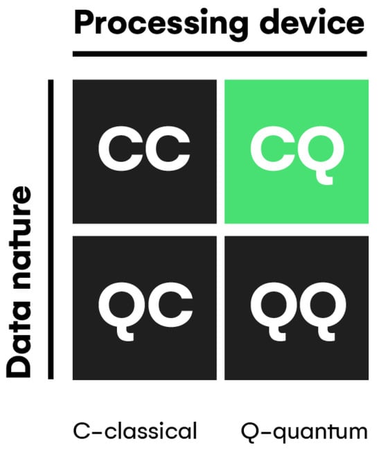
Figure 6.
Classical data on quantum algorithms.
- Python programming language (https://colab.google/articles/py3.10 (accessed on 23 April 2025)) used to develop calculations.
- Numpy, Pandas, Matplotlib, Seaborn, Scikit-learn and Sklearn (https://scikit-learn.org/stable/install.html (accessed on 23 April 2025)).
- IBM’s Qiskit and Qiskit Machine Learning provides the framework structure for developing QML.
- TensorFlow contains the platform structures for developing CML methods.
The calculations and results were obtained on a HP Probook (HP, London, UK) 645 G4 (AMD Ryzen 5 PRO (Ryzen, London, UK) and 20 Gb of RAM).
3.1. Implementation Process
(Algorithm 1) generates a disparity map, giving an overview of the logic and structure used in the implementation process of comparing CML and QML models.
| Algorithm 1: Compute Disparity Map |
 |
3.1.1. Dataset Description
The first step of the implementation process is to obtain an accurate and complete dataset as well as to guarantee that the classifiers perform well on unseen data by having a varied blend of malicious and benign URLs. The dataset [32] is made up of features gathered from various websites, utilized to categorize websites as malicious or benign. Additionally, the dataset contains unprocessed and unstructured HTML pages with JavaScript code, which can be employed as “unstructured data” for ML and DL and were collected by utilizing the MalCrawler tool to crawl the internet in order to find the data. The validation of labels in the dataset was performed with Google Safe Browsing and features were chosen depending on the significance each feature holds regarding how effectively they predicted both benign and malicious webpages in earlier studies conducted. The dataset consists of 1.2 million URLs with 11 main features (Table 2), with the last feature describing whether or not the URL is malicious. The description of features present in the dataset is given in the table below:
Table 2.
Feature descriptions of the dataset.
The dataset contains lexical, content and host-based or network features required in studying malicious websites, as each of these features provides distinct and valuable data that can boost the precision and resilience of detection algorithms.
3.1.2. Data Exploration
This stage aids in choosing the problem-solving strategy of data after an investigation has been conducted to find patterns and anomalies in the data. Before data exploration began, the dataset for this research was 1.2 million, which caused computational inefficiency when processing algorithms or multiple iterations as well as training models and exceeded the memory and storage capacity provided by the computer that the implementation process was conducted on. Consequently, this led to a reduction in the size of the data to be utilized by creating a subset of data containing 5000 instances, which is a well-recognized and supported strategy used in academic research [33]. The stratified sampling technique was used to create the new subset of data because, when working with heterogeneous datasets where several subgroups or strata within the data have unique characteristics whilst maintaining data integrity [34], this sampling technique is very effective.
Handling Missing Values
In the initial stage of exploring data, addressing any missing values in the dataset is vital for preserving the integrity of the dataset, as missing variables may introduce biases and diminish the statistical ability to conduct a thorough analysis. It was established that there were no missing data values in the dataset after a thorough examination. As a result, there was no requirement to impute or drop missing data, serving as a foundation for further exploration.
Descriptive Statistics
Moving on, the newly created dataset continues undergoing data exploration, starting with determining the descriptive statistics for each numerical variable in the dataset. These statistics provided a basic descriptive understanding of the data’s distribution, which included the following:
- Count: the quantity of values that are not missing for every variable, verifying the sample size of each calculation.
- Mean and Median: to evaluate any important differences that might point to skewness by comparing the central tendency measures.
- Standard Deviation and Variance: to assess the distribution of data.
- Minimum, Maximum and Range: to understand the entire range of data distribution.
Visualization of Data Distribution
To complement the descriptive statistics, data were visualized using graphical techniques, including histograms and box plots for numerical attributes and bar plots for categorical attributes (refer to Appendix B for categorical data graphs), to understand the shape of data distribution and capture other data qualities that the descriptive statistics may not have captured. This also aids in detecting skewness, which can be positive or negative, identifying outliers (data points that deviate significantly from the rest of the data) and comparing distribution across groups.
Correlation Analysis
A correlation heatmap visualization Figure 7 was used to understand the relationships between numerical variables and how each variable relates to others in order of identifying multicollinearity (highly correlated) and dependencies, especially for LR classifiers. Pearson’s correlation coefficient, also called PCC, was used for the analysis. PCC is a statistical measure that assesses the direction and strength of a linear relationship between two continuous variables, and [35] indicated that “the complexity of Pearson correlation is linear, making it efficient”. it ranges from −1 to 1 as follows:
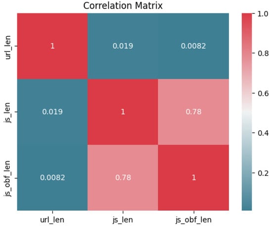
Figure 7.
Correlation plot for numerical features.
- −1 represents a perfect negative linear relationship;
- 0 represents no linear relationship;
- 1 represents a perfect positive linear relationship.
The formula for Pearson’s correlation is as follows:
where and denote the individual sample points and and denote the “mean of all records in features” X and Y, respectively.
3.1.3. Data Preprocessing
This stage ensures that data are clean, transformed and organized before applying the models from CML and QML. Pre-processing was performed through the following stages:
Encoding Categorical Variables
Categorical variables in datasets are frequently required to be converted to numerical formats for ML algorithms. Categorical variables including ‘url’, ‘geo_loc’, ‘tld’, ‘who_is’, ‘https’ and ‘label’ were converted to numerical values using the label encoder, which assigns each category variable a distinct integer. This approach of label encoding is particularly useful when categorical data is ordinal and the category order is significant. The categorical variables of the dataset were successfully converted to numerical, as shown in Figure 8, ensuring that the results will be compatible with any further analysis to be conducted.
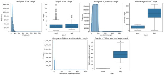
Figure 8.
Uni- variateplots for numerical features.
Handling Outliers
Outliers can significantly skew the results of data analysis, leading to incorrect models and predictions. In the box plot conducted for ‘url_len’, ‘js_len’ and ‘js_obf_len’, the level of outliers where the ‘good’ in the label group is high along with its corresponding label ‘bad’ being low, and vice versa, was observed for each of the individual attributes. These outliers are extreme values that deviate significantly from the rest of the data, potentially affecting the performance of ML models. The capping technique was used to reduce the influence of anomalies by substituting the percentile value for outliers. This technique effectively manages excessive values without eliminating essential data features. The first percentile (0.01) and the 99th percentile (0.99) for the lower and upper caps, respectively, were techniques applied to the columns mentioned above. This result improves data quality and model performance by putting extreme outliers in the data within a reasonable range while preserving most of the original data. It does this by capping all values below the 1st percentile to the 1st percentile value and all values above the 99th percentile to the 99th percentile value. Figure 9 shows a box plot of before capping and after applying capping techniques.
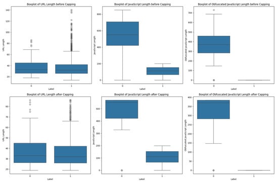
Figure 9.
Handling outliers.
Feature Scaling
Preparing data to be trained by ML models employs the scaling of features, as these models are sensitive to the magnitude of the input features. The feature scaling method utilized in this process is standardization, which modified the data to have zero (0) mean and one (1) standard deviation, as described in the descriptive statistics earlier on. This technique is essentially important especially when working with SVM classifiers. As mentioned, SVMs work by finding an optimal hyperplane that best separates different classes in a dataset, relying on the geometry of the feature space to classify data. When there are different units or scales in features, their variances can significantly affect the performance of SVMs. Standardization ensures that each feature contributes equally to calculations by centering the data while maintaining overall distribution, unlike min–max normalization, which will reduce most of the data into a small interval, ensuring that every component has the same scale but fails to handle outliers adequately. Furthermore, it was proven that standardization seemed to be the most effective scaling strategy for large and medium data sets of models such as SVMs, according to the experimental findings during a comparative analysis identifying when to use standardization and normalization [36].
Feature Selection
To further analyze, principal component analysis (PCA) was used to examine the dataset’s structure in more detail and identify the optimal number of components. PCA is an approach to reduce high dimensionality while maintaining as much variance (covariance of the entire set of patterns) as possible, leading to selecting certain features, if required, which was necessary for the current dataset in use. Following that, to enhance the model’s output performance, it was important to select the most relevant features of the dataset from the results of a scree plot. The analysis of variance (ANOVA) determines the most significant features contributing to the output variance. Theoretically, ANOVA is a collection of statistical methods utilized to identify the most significant features, especially when working with continuous independent variables and categorical dependent variables. It is effective when finding the “difference of means of two or more groups at the same time” [35]. According to [17], the statistical formula of ANOVA is given as follows:
where between groups is represented by (where k is the number of groups) and within groups is represented by (where N is the total number of observations). The application of the ANOVA test on a preprocessed dataset determines the relevance of the input variables and PCA selects the most relevant features [37]. Based on the ANOVA F-value score, the SelectKBest chose the top five features (5-component) with the best characteristics to be ‘tld’, ‘who_is’, ‘https’, ‘js_len’ and ‘js_obf_len’, with ‘label’ set as the target variable, thus reducing dimensionality in the dataset. Figure 10 below displays the scree plot of chosen features as all components capture a variance of 100%, which is sufficient for applications.
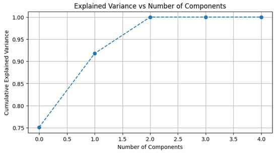
Figure 10.
PCA plot selected features.
Augmentation
The dataset was heavily imbalanced, with the majority class being ‘good’ (non-malicious/benign URLs represented as 1) and the minority class ‘bad’ (malicious URLs represented as 0). Utilizing this dataset to detect malicious URLs can skew the results of the training by becoming biased towards the majority class, thereby leading to an underrepresentation of the minority class and misleading performance metrics. To address this issue, a resampling techniques called oversampling and undersampling were utilized to achieve a balanced dataset. Oversampling randomly duplicates the minority class by replicating the samples in that class and undersampling randomly reduces the majority class samples, hence creating two separate datasets with different numbers of instances but with balanced classes. Instances of datasets undersampling and oversampling were later used in the classification and detection of malicious URLs in CML and QML techniques.
3.1.4. Model Architecture
SVM
Most importantly, SVM algorithms aim in seeking the hyperplane that best separates the classes (malicious versus non-malicious/benign URLs). This study, for parameter tuning, used the linear and RBF (radial basis function) kernel functions during experimentation for SVM classification.
- Linear kernel for linearly separable data.
- RBF kernel for non-linear data by mapping data into high-dimensional space.
The regularization parameter C was used, with values set as [0.1, 1, 10, 100, 1000] on both kernels to choose the right value for balancing bias and variance in the model. In continuation, the coefficient Gamma, a parameter specifically added to the RBF kernel to define the extent of influence for a single training, was set with values [0.001, 0.0001].
CNN
Although the CNN is mostly used for image classification and audio processing, it can be used to categorize numerical data when passed through the right sequence. This study used a two-dimensional CNN (2D-CNN) commonly applied to sequential data, where input from the dataset is reshaped to a tensor and treated as a two-dimensional sequence that can be easily fed to a CNN model. The dataset was converted into a 4D tensor of shape (an array of 3D) with the shape as (batch_size, height, width, channels), where height and width represent the dimensions of the input samples, batch_size is the number of samples in an input batch and channels is the number of input channels, denoted as 1. In building the CNN architecture, also called a ConvNet, each sequence of layers below was used to build a model that best fits the dataset in order to produce good performance in detecting malicious URLs.
- Convolutional Layers: Three 2D matrix convolutional layers were used to extract features from the dataset, for moving across the sequence. The first layer was assigned 32 filters/kernels and the latter two were assigned with 64, with all three layers given a sequence length of (1, 1).
- Activation Functions: The ReLU (rectified linear unit) function was used in this model for its efficiency in handling non-linearity in the network.
- Pooling Layers: A layer of max pooling was added to minimize the size of volume, which speeds up computation to save memory, therefore reducing computational cost and preventing overfitting.
- Flattening: Layer added to convert features from 2D matrix into 1D vector.
- Fully Connected Layers: This layer included two dense layers with activation functions, softmax and relu, to perform classification.
QSVM
QSVMs are quantum extensions of SVMs that provide an effective and natural framework for linear operations with the inclusion of those required for SVM computations. SVMs are best known for using kernels methods, likewise with QSVMs. The fundamental concept of quantum kernel machine learning (QKML) is to utilize quantum feature maps to carry out kernel techniques. A common kernel learning algorithm like the SVM algorithm can be integrated with quantum Kkernels (QKs) or, in addition, be used in a recently generated QK like the QSVC class.
QKs also require the use of quantum states and entanglement to extract and capture more complex relationships in the data. This research for QSVM classification utilized a QK simulator called Fidelity Quantum Kernel with the ZZ Feature Map for data encoding (transferring original data to qubits) and the parameterizing of quantum circuit set to a linear entanglement of both undersampled and oversampled datasets. Plugging QK into a classical method (SVC algorithm), kernel as a callable function and precomputed kernel matrix methods (SVC callable kernel and SVC precomputed kernel matrix) were used, proceeding to utilize the QSVC function to determine which model works better.
- Feature Mapping: ZZFeatureMap with entanglement set as linear. The feature mapping is given by
- Kernel Computation: The kernel computation is defined as
QCNN
This study extensively parameterized classical data classification utilizing QCNN. QCNN, like the classical CNN, processes data by integrating quantum circuits, which can improve the model’s capacity to identify patterns. The QCNN architecture is structurally similar to the classical CNN but replaces each classical operation with its quantum counterpart. Undersampled and oversampled datasets were encoded using the ZFeatureMap and proceeded to define and build Ansatz (including trainable weights), forming a quantum neural network (QNN) circuit.
- Quantum Convolutional Layers: A total of two convolutional layers were used to apply a series of quantum gates defined in the layer function to the quantum state, to effectively extract features in the quantum space.
- Quantum Pooling Layers: A total number of two pooling layers were used from a defined function to reduce the number of qubits by applying controlled measurements or quantum operations whilst still preserving relevant information.
The feature map and Ansatz are combined and plugged into the QNN function alongside the measurement output loss function of trainable weights through backpropagation.
3.1.5. Training and Testing Procedures
Data Splits
The datasets were divided into training and testing sets with a ratio of 80:20 for both the CML and QML models and cross-validated using k-fold (10-fold in the actual program, where CV equals 10) for CML models. This process guarantees that the model is tested on unseen data to determine how effectively it generalizes.
Training Process
- SVM: Grid Search was utilized to find the optimal C and kernel parameters for both undersampled and oversampled datasets.
- CNN: Random search was used to optimize the number of filters, kernel size, and dropout rate, with epochs set at 10. The optimizer used was Adam, and the loss function was set to categorical_crossentropy.
- QSVM: training with SVC callable, SVC precomputed and QSVC functions.
- QCNN: trained the classifier utilizing the COBYLA optimizer often employed for numerical optimization and Pauli-Z expectation values as measurement.
3.1.6. Evaluation Matrix
There are matrix terms that need to be understood, as this allows the visualization of the performance of an algorithm by comparing the predicted class against the actual class. For a confusion matrix, there are four key metrics:
- True Positives: TP, the number of instances correctly predicted as positive (malicious).
- True Negatives: TN, the number of instances correctly predicted as negative (benign).
- False Positives: FP, the number of instances incorrectly predicted as positive when they are actually negative.
- False Negative: FN, the number of instances incorrectly predicted as negative when they are actually positive.
This confusion matrix is now interpreted using accuracy, precision, recall or sensitivity and F-score.
Accuracy: This gives the ratio of correctly predicted instances to the total number of instances (TNI). It is calculated as
Precision: This gives the ratio of correctly predicted positive observations to the total predicted positives. It is calculated as
Recall (Sensitivity): This gives the ratio of correctly predicted positive observations in the actual class. It is calculated as
F-score: This gives the harmonic mean of precision and recall by providing a single metric that balances both precision and recall. It is calculated as
4. Data Analysis and Critical Discussions
4.1. Model Performance
This section provides a detailed analysis of the performance of the SVM, QSVM, CNN and QCNN models used in this experiment and their outcomes.
4.1.1. Data Class Imbalance
These models were evaluated using both undersampling and oversampling techniques to correct the data imbalance of the original dataset as shown in (Figure 11). When classes are not equally represented (skewed distribution) in a dataset, it can cause models to produce biased predictions from labelled classes. This imbalance may result in a model being biased towards predicting the majority class, thereby reducing the ability to detect the minority class, hence producing an ineffective model that can gain good scores for accuracy but not for precision, recall and f scores. Resampling techniques are used to effectively ensure class imbalance is handled, which involves undersampling the majority class and oversampling the majority class.
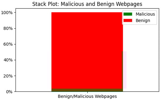
Figure 11.
Class label distribution.
Respectively, the variations of the techniques are random undersampling (RUS) and random oversampling (ROS) (Table 3). In a systematic review conducted by [38] the authors discovered that resampling approaches were used in “156 out of 527” papers or “29.6” percent of all articles to solve data imbalance issues in a minimum of 12 fields. Additionally, Ref. [39] used 104 datasets for the comparison and evaluation of 85 oversampling strategies. Both studies demonstrated how much research has been conducted in the current literature on the potentiality of resampling addressing problems from class imbalance. The competence of each resampling technique is dependent on “the imbalance ratio between the class target variable” and its operational principle. For instance, when applied to slightly imbalanced data, oversampling is seen as an effective technique compared to undersampling, which is more effective when applied to highly imbalanced data [40]. However, having this theory in mind, when comparing the overall output performance of the models in Table 4 and Table 5, it is clearly seen that oversampling the minority class generated better results than undersampling the majority class, hence disproving the theory.
Table 3.
The comparison of resampling techniques utilized.
Table 4.
Performance metrics for undersampling models.
Table 5.
Performance metrics for oversampling models.
Table 6 shows the time taken to train and test both RUS and ROS. It is evident and safe to say that RUS has a decreased training and testing time of predictive models as compared to ROS, which has relatively increased training and testing times of predictive models. Ref. [40] further discussed that training time may cause underfitting in RUS due to shorter training times and overfitting in ROS due to longer training times. Overfitting occurs when an ML model learns the training data excessively well due to longer training times; as a result, it overfits and captures detail or noise that does not generalize well to unseen data. This occurrence usually happens when too many parameters are used relative to the amount of training data. Meanwhile, underfitting occurs when ML models have insufficient data and time in the training process, hence leading to a poor performance on both training and testing data. To overcome overfitting and underfitting, k-fold cross validation and epochs were used. Cross validation was set to 10, meaning that the 10-fold cross-validation divided each dataset into 10 parts. The model trained on nine parts and tested on the 10th part and repeated the process 10 times, with each part taking a turn as the validation set. Epochs were also set to 10, where the model processed every sample in the training set once and the model’s weights were updated accordingly until it reached the 10th epoch.
Table 6.
Training and testing time for undersampling and oversampling models.
4.1.2. Performance Analysis
This section analyzes the table and graphs to discuss which model performs best overall.
SVM
SVM with a linear kernel and an RBF kernel was applied to both undersampled and oversampled datasets.
- SVM Linear Kernel
SVM with a linear kernel was applied to the undersampled dataset (Figure 12); the model was able to correctly classify 97.87 percent of the instances, with a perfect precision score, which indicates no false positives, and a high recall, which suggests that the minority class instances (being malicious/bad/0) were correctly identified. Given that the data most likely had a linear separability after undersampling, referring to a situation in which the lower complexity of the data enabled the SVM model to quickly identify the optimal separating hyperplane, the linear kernel in this situation was made more suitable.
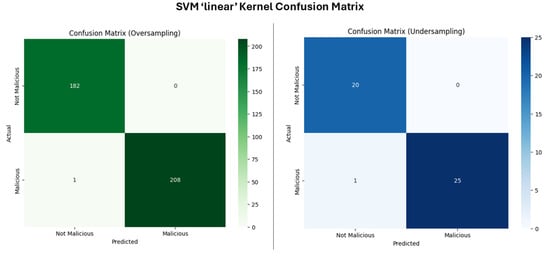
Figure 12.
Confusion matrix for SVM linear.
When the linear kernel was applied to the oversampled dataset, the SVM linear kernel model continued to perform well in accuracy but with a near perfect precision and recall, suggesting most of the majority (being benign/good/1) class instances were correctly identified. The model maintained high accuracy in classifying both classes correctly, with zero false positives and one false negative. The near-perfect outcome demonstrates that the linear kernel was an appropriate fit for the oversampled data, where the insertion of synthetic minority class samples did not significantly alter the decision boundary.
- SVM RBF Kernel
The RBF kernel is commonly known for handling non-linear relationships within the data, hence making it suitable for more complex datasets where linear separation is not feasible. For the undersampled dataset (Figure 13), there is a slightly lower accuracy and recall when compared to the linear kernel, which implies that while the RBF kernel was able to model the decision boundary effectively, it may seem overfitted to the undersampled dataset. Non-linear kernels, such as the RBF in SVMs, frequently carry this risk, especially when the dataset is reduced, because the model may become “too finely tuned” to the limited examples [41]. The higher number of false negatives compared to the linear kernel implies that the RBF model was slightly less effective at identifying all instances of the malicious class.
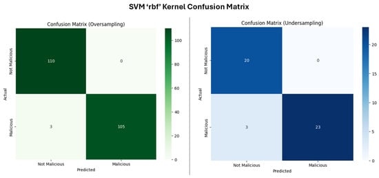
Figure 13.
Confusion matrix for SVM RBF.
For the oversampled dataset, the RBF kernel displayed improved general output performance in comparison to the undersampled dataset but not with the linear kernel oversampled dataset as it had higher false negatives, failing to identify the malicious instances. The significant improvement for the undersampled dataset is attributed to the additional data provided by the oversampling technique, which allowed the kernel to better generalize the decision boundary without overfitting.
QSVM
The focus of this section was to utilize a QML technique called fidelity quantum kernel (FQK) methods applied on classical data. The process of feature map where a “parametrized quantum evolution (usually parametrized quantum circuit)” is utilized in FQK techniques to encode a classical data “point in a quantum state” [42]. The objective of the encoding for classical kernel techniques is to facilitate data analysis. Ref. [41] further discussed that a paired measure of similarity using the encoded points of data (i.e., “the fidelity of two encoded quantum states”) provides the kernel function, hence the paired similarities “between input data points” make up the kernel matrix. Afterwards, the FQK can then be applied to classification utilizing classical kernel machines like SVM. ZZFeatureMap encoded the data to correlate the number of qubits and number of features in the classical dataset used to compute the kernel, measuring the similarity between data points; then, the QSVM uses this quantum kernel to separate data points into different classes just like the classical kernels in SVM. The advantage of utilizing ZZFeatureMap is to construct a highly expressive and non-linear feature space where data points that are not linearly separable in the original space may become linearly separable [28], hence leading to a better classification performance, especially on classical datasets, to comprehend patterns. (Figure 14) shows the feature map obtained for this study.
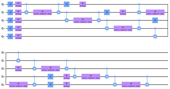
Figure 14.
ZZFeatureMap circuit for QSVM.
For the first two implementations for QSVM, the FQK was connected to the classical kernel method known as the SVC algorithm, which allows the algorithm to define a custom kernel by rendering the kernel available as a callable function (QSVM CK) and employing the kernel as a precomputed kernel matrix (QSVM PK), hence using the kernel.evaluate function in the algorithm. The later implementation used a variation of SVC called the QSVC function that accepts the FQK as input rather than evaluating it.
- SVC Callable Kernel
The QSVM CK (Figure 15) achieved a perfect score on all measures in both undersampled and oversampled datasets, demonstrating an outstanding performance. This further indicates that the ZZFeature map allowed an ideal separation of classes and the FQK was highly effective in capturing relevant features of the data even with undersampling.
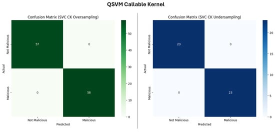
Figure 15.
Confusion matrix for QSVM CK.
- SVC Precomputed Kernel
Similar to QSVM CK, QSVM PK (Figure 16) achieved a perfect classification in both undersampled and oversampled datasets, with high TPs and TNs.
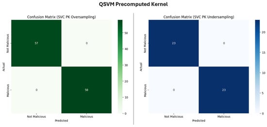
Figure 16.
Confusion matrix for QSVM PK.
- QSVC Function
Similar to QSVM CK and QSVM PK, the QSVC (Figure 17) also achieved a perfect classification in both undersampled and oversampled datasets, with also high TPs and TNs.
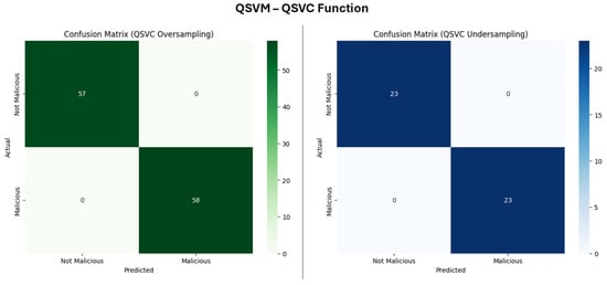
Figure 17.
Confusion matrix for QSVM Func.
CNN
The CNN model, when applied to the undersampled dataset, demonstrated a near perfect performance, though not one as perfect as the previously mentioned models. The CNN model (Figure 18) achieved an accuracy of 91.30 percent, indicating that it correctly classified over 91 percent of the instances. The precision of 95.83 percent suggests that the model wrongly made a false positive prediction (flagging one benign class as malicious) and recall of 88.46 percent shows that model failed to detect three malicious instances.
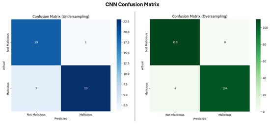
Figure 18.
Confusion matrix for CNN.
Looking at the oversampled dataset result, the performance of the CNN slightly improved with an accuracy of 99.90 percent and precision of 100 percent, indicating that the model correctly classified nearly all instances without a false positive prediction but still failed in detecting four malicious instances. However, (Figure 19) suggests that the CNN model learned effectively after the numerical dataset was reshaped to satisfy the input sequence of the CNN.
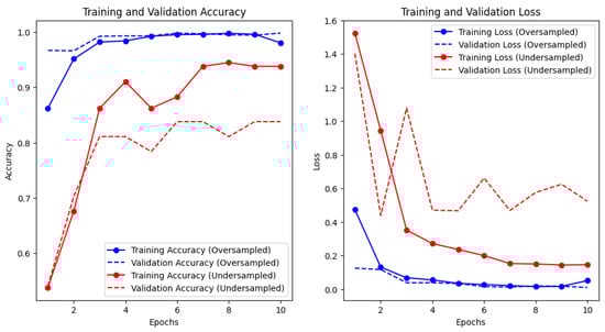
Figure 19.
Training and validation for accuracy and loss in CNN.
The oversampled dataset shows a more consistent performance between training and validation, which indicates a better generalization, with the high and stable accuracy suggesting that the model was learning the patterns well without overfitting. In contrast to the oversampled dataset, the undersampled dataset shows a gap in training and validation accuracy, where the gap indicates a sign that the model might be overfitting to the training data, especially since the training accuracy is higher than the validation accuracy. (Figure 19) shows a good learning curve where both training and validation loss decrease and stabilize with minimal difference between the two, hence indicating that the model was well trained and likely to generalize well to new data. The undersampled dataset, in the same manner as the left plot, showed a larger and more erratic gap between training and validation loss, with validation fluctuating and decreasing as consistently, thereby suggesting that the model is learning the training data well but struggling to generalize to unseen data, likely due to the model being trained on fewer instances, so it did not see enough variation to learn general patterns in the study.
QCNN
Similarly to QSVM, datasets in QCNN were encoded by applying ZFeatureMap, designed to process input data to quantum states in QNN. [6] experimented using ZFeatureMap (Figure 20) and the COBYLA optimizer, which significantly reduced the training time of training data. ZFeatureMap with the combination of a parametrized circuit (Ansatz) and an optimizer yielded a promising result when compared to other feature maps used in the experiment to detect malicious URLs using VQC. In the QCNN model, the EstimatorQNN was used in the model to process the quantum states through a series of two quantum convolutions and pooling. The NeuralNetworkClassifier operates on the features extracted by the quantum layer through the EstimatorQNN and makes the final decision-making layer by taking the quantum-processed data and applying it to a classical learning algorithm to classify data points. This overall approach uses quantum circuits for feature extraction and classical networks for classification.
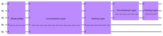
Figure 20.
ZFeatureMap circuit of model in QCNN.
The QCNN model on the undersampled dataset achieved a moderate performance (Figure 21) where recall rate indicates that the model was fairly effective at identifying the malicious class; however, it wrongly flagged five benign instances as malicious and the model failed to detect two malicious instances and classified the two instances as benign. Similarly to with the oversampled dataset, the model wrongly flagged 13 benign instances as malicious and also failed to detect four malicious instances, classifying them as benign.
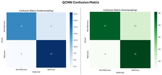
Figure 21.
Confusion matrix for QCNN.
However, Figure 22 below shows that the process of tuning the parameters of the quantum circuits to minimize a loss function related to the classification accuracy was successful due to the convergence displayed in the plot. This indicated that although the model did not achieve promising results, the model learned the effective way to represent and classify the input data.
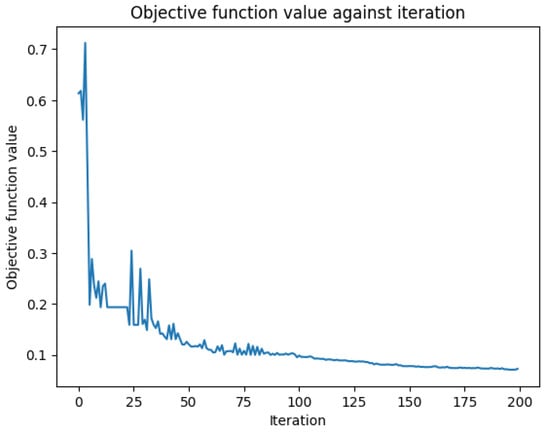
Figure 22.
Loss function in QCNN.
4.2. Comparison of CML and QML Models
The experimental results demonstrated clear performance differences between the quantum-enhanced and classical machine learning models in detecting malicious URLs. The QSVM consistently outperformed the SVM in both undersampled and oversampled datasets, with perfect scores in accuracy, precision and recall. This superior performance can be attributed to the QSVM’s fundamental quantum mechanical advantages. Unlike classical SVM kernels, which operate in limited feature spaces, the QSVM utilizes quantum feature mapping (specifically the ZZFeatureMap) to project the input data into an exponentially higher dimension. Classical SVM kernels might overlook complex non-linear and subtle feature interactions, but quantum-enhanced features enable the model to identify and leverage them. With the quantum entanglement properties built into the circuit design, complex relationships between seemingly unrelated URL characteristics such as ‘js_obf_len’ and ‘tld’ domain patterns can be captured by QSVM, while CML models might treat them as independent features. In contrast, the comparison between the CNN and QCNN revealed a different performance dynamic, with the CNN outperforming the QCNN in this experiment, especially in the oversampled dataset, particularly when the CNN obtained an accuracy of 99.90 percent versus the QCNN obtaining 85.22 percent. CNNs, while originally designed for image processing, can be effectively adapted for sequential and numerical data through appropriate tensor reshaping. The CNN’s multi-layer hierarchical structure enables it to learn representations of URL features ranging from lexical patterns to combinations of network and content characteristics. The presence of established optimization methods and widely understood architectures adds to the model’s performance. Meanwhile, the performance of the QCNN may be attributed to quantum neural networks primarily designed and optimized for image-like structures that can be naturally stored in qubits, making it unsuitable for the numerical data used in this experiment. Additionally, the field of quantum deep learning is still developing effective training methodologies and their practical application tasks require further research. Figure 23 and Figure 24 present a performance evaluation for the models.
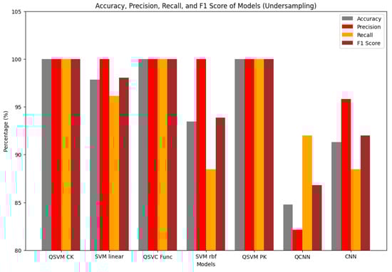
Figure 23.
Performance comparison for all models in the undersampled dataset.
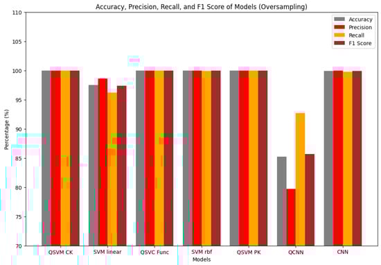
Figure 24.
Performance comparison for all models in the oversampled dataset.
4.3. Challenges Faced on Models
Whenever it comes to practical applications in cybersecurity, particularly related to detecting malicious URLs, speed and accuracy are crucial, hence the need for computational efficiency in assessing the practicality of ML models. CML models demonstrated a much faster time in both training and testing times compared to QML models, as shown in Table 6. The QSVM achieved perfect classification. However, its implementation faces practical limitations due to current quantum hardware constraints, operating only on simulators rather than actual quantum processors. The QCNN demonstrated potential but faced significant theoretical and practical limitations as it is designed for quantum data structures and, therefore, struggles with classical numerical data processing. The field also lacks mature training methodologies possessing current quantum hardware restrictions. CML models currently hold an advantage because CML models have been thoroughly researched and optimized for years, with an abundance of practical experimentation on this subject and many other fields. However, as quantum computing advances, the gap in computational efficiency is expected to be narrowed, potentially giving QML models an edge in future applications, especially given the results obtained from the QSVM.
5. Conclusions and Future Work
This study has provided a comprehensive analysis of malicious URL detection through both classical and quantum machine learning (QML) techniques. A thorough review of traditional detection strategies set the foundation for an in-depth comparative study of supervised, unsupervised and deep learning methodologies. Additionally, the study explored the emerging domain of QML and evaluated its potential to enhance cybersecurity. Methodologically, both quantitative and qualitative approaches were employed, ensuring the dataset was pre-processed to maintain the integrity and validity of each model’s performance. The comparative analysis revealed critical insights into the current strengths and limitations of both classical and quantum learning models. While classical machine learning (CML) models such as support vector machines (SVMs) and convolutional neural networks (CNNs) remain effective for practical applications, quantum models, particularly quantum SVMs (QSVMs), demonstrated substantial promise in advancing cybersecurity methodologies.
5.1. Unexpected Findings
One of the most unexpected discoveries in this study was the perfect performance of the QSVM, achieving accuracy, recall and precision across all classification types using both undersampled and oversampled datasets. Although previous research has suggested that QML models have the potential to surpass classical counterparts, the exceptional results obtained in this study were unanticipated, given the current limitations of quantum computing (QC), particularly in hardware and software capabilities.
Additionally, the study yielded insights into the performance of the CNN and the QCNN on numerical datasets. While the CNN successfully adapted to the reshaped numerical dataset by leveraging multi-dimensional tensor transformations, the QCNN struggled to classify non-image data effectively. This suggests that classical CNN models may still hold an advantage in handling structured numerical datasets, whereas QCNNs require further refinement.
5.2. Theoretical and Practical Implications
The findings from this research contribute to the growing body of evidence supporting QML’s potential to outperform CML in specific tasks. The superior performance of QSVM reinforces the expressiveness of quantum feature spaces, demonstrating that quantum kernels may provide a more powerful alternative to classical kernels. This aligns with foundational QC principles, particularly the advantages of quantum entanglement and parallelism in handling complex computational problems.
From a practical perspective, the demonstrated efficacy of QSVM carries significant implications for cybersecurity. If quantum computing infrastructure stabilizes and becomes more accessible, QSVM could be integrated into real-world applications for detecting and mitigating cyber threats. This underscores the necessity of continued investment in quantum hardware development, particularly in extending quantum coherence times, reducing error rates and increasing qubit counts to fully harness QML’s capabilities.
5.3. Challenges and Limitations
Despite the promising results, this study faced several challenges and limitations. One primary limitation was dataset augmentation, which, although useful for addressing class imbalance, posed the risk of introducing erroneous patterns that could lead to overfitting. Additionally, computational constraints posed a significant hurdle during the experimental phase. The study relied on Google Colab, which had limitations in handling extended training times for oversampled datasets. To mitigate this, a fraction of the dataset was used—one ninth (1/9) for SVM linear and one seventeenth (1/17) for QSVM and QCNN—to reduce the training time and avoid runtime errors. This study used quantum simulators (which are not real quantum hardware), which do not suffer from noise, but in real-world deployments, studies show that noise would introduce errors in calculations, reducing model accuracy.
5.4. Ethical Considerations for Quantum Computing in Cyber Security
Quantum computing has the potential to significantly improve defensive cybersecurity measures, such as breaking existing encryption (Shor’s algorithm) or enhancing threat detection through QML. Malicious actors, state-sponsored hackers or cybercriminal groups, on the other hand, could use these capabilities to their advantage. Policymakers and researchers must balance innovation with safeguards to prevent quantum computing from becoming a destabilizing force in cyber warfare. Secondly, QML may enable hyper-efficient data analysis, increasing intrusion detection while creating privacy concerns. Governments or corporations with quantum computing capability may use it to conduct mass surveillance under the pretense of cybersecurity, analyzing encrypted communications or behavioral patterns on unprecedented scales. Ethical frameworks must control quantum-enhanced surveillance to prevent abuses of power while also assuring compliance with data protection rules such as GDPR. Additionally, QML models are fundamentally less accessible than classical algorithms due to their reliance on quantum superposition and entanglement. If a quantum model falsely flags a benign URL as malicious or fails to detect a real threat, tracing the decision-making process is difficult. This “black box” problem raises ethical concerns about accountability, particularly in high-stakes cybersecurity applications where errors could lead to financial losses or infrastructure failures. Developing explainable quantum AI frameworks is critical for maintaining trust and transparency.
5.5. Future Work
Future research should aim to address these computational constraints by leveraging more advanced quantum computing resources to test on larger and more complex datasets. Further exploration into alternative quantum algorithms, feature maps, kernels and optimization techniques could enhance the efficiency of binary and multi-class classification for malicious URL detection. Researchers should systematically investigate novel quantum feature mapping techniques beyond the current ZZFeatureMap approach. Moreover, considering the performance gap between CNNs and QCNNs, future studies could investigate transforming numerical datasets into grayscale images and training them with advanced CNN architectures such as GoogleNet and ResNet50, which have shown success in complex classification tasks. Such advancements will be instrumental in refining quantum-based cybersecurity solutions and expanding their applicability across various domains.
Author Contributions
U.B.C.: Conceptualization, Resources, Writing—review and editing, Supervision, Funding acquisition. L.E.: Methodology, Validation, Formal analysis, Investigation, Data curation, Writing—original draft. H.J.: Visualization, Supervision, Project administration. All authors have read and agreed to the published version of the manuscript.
Funding
This research received no specific grant from any funding agency in the public, commercial or not-for-profit sectors.
Informed Consent Statement
All authors give consent for the publication of identifiable details, which can include photograph(s) and/or videos and/or case history and/or details within the text to be published in the above journal and article.
Data Availability Statement
The data that support the findings of this study are available from the corresponding author, Umair B. Chaudhry, upon reasonable request.
Conflicts of Interest
All authors declare that they have no conflicts of interest.
References
- Hong, J. The State of Phishing Attacks. Commun. ACM 2012, 55, 74–81. [Google Scholar] [CrossRef]
- Liang, B.; Huang, J.; Liu, F.; Wang, D.; Dong, D.; Liang, Z. Malicious Web Pages Detection Based on Abnormal Visibility Recognition. In Proceedings of the 2009 International Conference on E-Business and Information System Security, Wuhan, China, 23–24 May 2009. [Google Scholar]
- HACKMAGEDDON. 2024 Cyber Attacks Statistics–HACKMAGEDDON. Available online: https://www.hackmageddon.com/category/security/cyber-attacks-statistics/ (accessed on 25 June 2024).
- Kar, A.K.; He, W.; Payton, F.C.; Grover, V.; Al-Busaidi, A.S.; Dwivedi, Y.K. How Could Quantum Computing Shape Information Systems Research–An Editorial Perspective and Future Research Directions. Int. J. Inf. Manag. 2025, 80, 102776. [Google Scholar] [CrossRef]
- Kalinin, M.; Krundyshev, V. Security Intrusion Detection Using Quantum Machine Learning Techniques. J. Comput. Virol. Hacking Tech. 2023, 19, 125–136. [Google Scholar] [CrossRef]
- Reyes-Dorta, N.; Caballero-Gil, P.; Rosa-Remedios, C. Detection of Malicious URLs Using Machine Learning. Wirel. Netw. 2024, 30, 7543–7560. [Google Scholar] [CrossRef]
- Aljofey, A.; Jiang, Q.; Rasool, A.; Chen, H.; Liu, W.; Qu, Q.; Wang, Y. An Effective Detection Approach for Phishing Websites Using URL and HTML Features. Sci. Rep. 2022, 12, 8842. [Google Scholar] [CrossRef]
- Prakash, P.; Kumar, M.; Rao Kompella, R.; Gupta, M. PhishNet: Predictive Blacklisting to Detect Phishing Attacks. In Proceedings of the 2010 Proceedings-IEEE INFOCOM, San Diego, CA, USA, 14–19 March 2010. [Google Scholar] [CrossRef]
- Felegyhazi, M.; Kreibich, C.; Paxson, V. On the Potential of Proactive Domain Blacklisting. LEET 2010, 10, 6. [Google Scholar]
- Sheng, S.; Wardman, B.; Cranor, L.; Hong, J.; Zhang, C. An Empirical Analysis of Phishing Blacklists. In Proceedings of the 6th Conference on Email and Anti-Spam (CEAS’09), Mountain View, CA, USA, 16–17 July 2009. [Google Scholar]
- Garera, S.; Provos, N.; Chew, M.; Rubin, A. A Framework for Detection and Measurement of Phishing Attacks. In Proceedings of the 2007 ACM Workshop on Recurring Malcode, Alexandria, VA, USA, 2 November 2007. [Google Scholar]
- Li, S.; Huang, T.; Qin, Z.; Zhang, F.; Chang, Y. Domain Generation Algorithms Detection through Deep Neural Network and Ensemble. In Proceedings of the Companion Proceedings of the 2019 World Wide Web Conference, San Francisco, CA, USA, 13–17 May 2019; ACM: New York, NY, USA, 2019; pp. 189–196. [Google Scholar]
- Sahoo, D.; Liu, C.; Hoi, S.C.H. Malicious URL Detection Using Machine Learning: A Survey. arXiv 2017, arXiv:1701.07179. [Google Scholar] [CrossRef]
- Saiful, M.; Mamun, I.; Rathore, M.A.; Lashkari, A.H.; Stakhanova, N.; Ghorbani, A.A. Detecting Malicious URLs Using Lexical Analysis. In Network and System Security: 10th International Conference, NSS 2016, Taipei, Taiwan, 28–30 September 2016; Springer: Berlin/Heidelberg, Germany, 2016. [Google Scholar] [CrossRef]
- Hu, Z.; Yuan, Z. A Review of Data-driven Approaches for Malicious Website Detection. In Proceedings of the 2023 7th Asian Conference on Artificial Intelligence Technology (ACAIT), Quzhou, China, 10–12 November 2023. [Google Scholar]
- Aljabri, M.; Altamimi, H.S.; Albelali, S.A.; Al-Harbi, M.; Alhuraib, H.T.; Alotaibi, N.K.; Alahmadi, A.A.; Al Haidari, F.; Mohammad, R.M.A.; Salah, K. Detecting Malicious URLs Using Machine Learning Techniques: Review and Research Directions. IEEE Access 2022, 10, 121395–121417. [Google Scholar] [CrossRef]
- Aljabri, M.; Alhaidari, F.; Mohammad, R.M.A.; Samiha, M.; Alhamed, D.H.; Altamimi, H.S.; Chrouf, S.M.B. An Assessment of Lexical Network and Content-Based Features for Detecting Malicious URLs Using Machine Learning and Deep Learning Models. Comput. Intell. Neurosci. 2022, 2022, 3241216. [Google Scholar] [CrossRef]
- Alfouzan, N.A.; Narmatha, C. A Systematic Approach for Malware URL Recognition. In Proceedings of the 2022 2nd International Conference on Computing and Information Technology (ICCIT 2022), Tabuk, Saudi Arabia, 25–27 January 2022; Institute of Electrical and Electronics Engineers Inc.: New York, NY, USA, 2022; pp. 325–329. [Google Scholar] [CrossRef]
- Cervantes, J.; Garcia-Lamont, F.; Rodríguez-Mazahua, L.; Lopez, A. A Comprehensive Survey on Support Vector Machine Classification: Applications, Challenges, and Trends. Neurocomputing 2020, 408, 189–215. [Google Scholar] [CrossRef]
- Chiramdasu, R.; Srivastava, G.; Bhattacharya, S.; Reddy, P.K.; Gadekallu, T.R. Malicious URL Detection Using Logistic Regression. In Proceedings of the 2021 IEEE International Conference on Omni-Layer Intelligent Systems (COINS 2021), Barcelona, Spain, 23–25 August 2021; Institute of Electrical and Electronics Engineers Inc.: New York, NY, USA, 2021. [Google Scholar] [CrossRef]
- Jain, A.K.; Gupta, B.B. A Machine Learning Based Approach for Phishing Detection Using Hyperlinks Information. J. Ambient Intell. Humaniz. Comput. 2019, 10, 2015–2028. [Google Scholar] [CrossRef]
- Ranganathan, P.; Pramesh, C.; Aggarwal, R. Common Pitfalls in Statistical Analysis: Logistic Regression. Perspect. Clin. Res. 2017, 8, 148. [Google Scholar] [CrossRef] [PubMed]
- Bu, S.J.; Cho, S.B. Deep Character-Level Anomaly Detection Based on a Convolutional Autoencoder for Zero-Day Phishing URL Detection. Electronics 2021, 10, 1492. [Google Scholar] [CrossRef]
- Saxe, J.; Berlin, K. eXpose: A Character-Level Convolutional Neural Network with Embeddings for Detecting Malicious URLs File Paths and Registry Keys. arXiv 2017, arXiv:1702.08568. [Google Scholar]
- Le, H.; Pham, Q.; Sahoo, D.; Hoi, S.C.H. URLNet: Learning a URL Representation with Deep Learning for Malicious URL Detection. arXiv 2018, arXiv:1802.03162. [Google Scholar]
- Siteefy. How Many Websites Are There in the World? (2024)-Siteefy. Available online: https://siteefy.com/how-many-websites-are-there/ (accessed on 15 July 2024).
- Mercaldo, F.; Ciaramella, G.; Iadarola, G.; Storto, M.; Martinelli, F.; Santone, A. Towards Explainable Quantum Machine Learning for Mobile Malware Detection and Classification †. Appl. Sci. 2022, 12, 12025. [Google Scholar] [CrossRef]
- Power, L.; Guha, K. Feature Importance and Explainability in Quantum Machine Learning. arXiv 2024, arXiv:2405.08917. [Google Scholar]
- Kak, S. On Quantum Neural Computing. Inf. Sci. 1995, 83, 143–160. [Google Scholar] [CrossRef]
- Li, Z.; Liu, X.; Xu, N.; Du, J. Experimental Realization of Quantum Artificial Intelligence. Phys. Rev. Lett. 2014, 114, 140504. [Google Scholar] [CrossRef]
- Mancilla, J.; Pere, C. A Preprocessing Perspective for Quantum Machine Learning Classification Advantage in Finance Using NISQ Algorithms. Entropy 2022, 24, 1656. [Google Scholar] [CrossRef]
- Singh, A.K. Malicious and Benign Webpages Dataset. Data Brief 2020, 32, 106304. [Google Scholar] [CrossRef] [PubMed]
- Gao, K.; Khoshgoftaar, T.M.; Napolitano, A. Combining Feature Subset Selection and Data Sampling for Coping with Highly Imbalanced Software Data. In Proceedings of the 27th International Conference on Software Engineering and Knowledge Engineering, St. Louis, MO, USA, 15–21 May 2005. [Google Scholar] [CrossRef]
- Sadaiyandi, J.; Arumugam, P.; Sangaiah, A.K.; Zhang, C. Stratified Sampling-Based Deep Learning Approach to Increase Prediction Accuracy of Unbalanced Dataset. Electronics 2023, 12, 4423. [Google Scholar] [CrossRef]
- Ahsan, M.; Gomes, R.; Chowdhury, M.M.; Nygard, K.E. Enhancing Machine Learning Prediction in Cybersecurity Using Dynamic Feature Selector. J. Cybersecur. Priv. 2021, 1, 199–218. [Google Scholar] [CrossRef]
- Sujon, K.M.; Hassan, R.B.; Towshi, Z.T.; Othman, M.A.; Samad, M.A.; Choi, K. When to Use Standardization and Normalization: Empirical Evidence from Machine Learning Models and XAI. IEEE Access 2024, 12, 135300–135314. [Google Scholar] [CrossRef]
- Sri Preethaa, K.R.; Munisamy, S.D.; Rajendran, A.; Muthuramalingam, A.; Natarajan, Y.; Abdi, A. Novel ANOVA-Statistic-Reduced Deep Fully Connected Neural Network for the Damage Grade Prediction of Post-Earthquake Buildings. Sensors 2023, 23, 6439. [Google Scholar] [CrossRef]
- Guo, H.; Li, Y.; Shang, J.; Gu, M.; Huang, Y.; Gong, B. Learning from Class-imbalanced Data: Review of Methods and Applications. Expert Syst. Appl. 2017, 73, 220–239. [Google Scholar] [CrossRef]
- Kovács, G. An Empirical Comparison and Evaluation of Minority Oversampling Techniques on a Large Number of Imbalanced Datasets. Appl. Soft Comput. 2019, 83, 105662. [Google Scholar] [CrossRef]
- Wongvorachan, T.; He, S.; Bulut, O. A Comparison of Undersampling Oversampling and SMOTE Methods for Dealing with Imbalanced Classification in Educational Data Mining. Information 2023, 14, 54. [Google Scholar] [CrossRef]
- Koziarski, M. Radial-Based Undersampling for Imbalanced Data Classification. Pattern Recognit. 2020, 102, 107262. [Google Scholar] [CrossRef]
- Slattery, L.; Shaydulin, R.; Chakrabarti, S.; Pistoia, M.; Khairy, S.; Wild, S.M. Numerical Evidence Against Advantage with Quantum Fidelity Kernels on Classical Data. Phys. Rev. A 2023, 107, 062417. [Google Scholar] [CrossRef]
Disclaimer/Publisher’s Note: The statements, opinions and data contained in all publications are solely those of the individual author(s) and contributor(s) and not of MDPI and/or the editor(s). MDPI and/or the editor(s) disclaim responsibility for any injury to people or property resulting from any ideas, methods, instructions or products referred to in the content. |
© 2025 by the authors. Licensee MDPI, Basel, Switzerland. This article is an open access article distributed under the terms and conditions of the Creative Commons Attribution (CC BY) license (https://creativecommons.org/licenses/by/4.0/).