Learning-Enabled Robust Control of Thermoacoustic Oscillations

Abstract

This work addresses the learning-enabled robust control of thermoacoustic systems under uncertainties and unknown disturbances. A widely recognized thermoacoustic system model is considered, incorporating monopole-like actuators and sensor arrays for demonstration. The model is reformulated into a set of ordinary differential equations (ODEs) suitable for control design. The learning-enabled control law is derived by minimizing a cost function that reflects the target closed-loop error dynamics using a gradient descent method. The closed-loop system stability is established through a pseudolinear system approach. The learning-enabled control law effectively mitigates the unwanted effects of uncertainties and disturbances. The controller performance is validated using a combustion system model featuring two modes and two actuators.

1. Introduction

Unwanted large-amplitude pressure oscillations in combustion systems can lead to significant performance deterioration. Such self-excited combustion oscillations represent a major challenge for aero-engine manufacturers [1,2,3]. To stabilize otherwise unstable thermoacoustic systems, two main approaches exist: passive and active control.

Passive control methods involve system redesign, such as altering the heat source position or using acoustic dampers and liners [4,5,6,7,8]. While passive approaches are straightforward, they lack adaptability to changing operating conditions. In contrast, active control methods dynamically adjust to variations in system behavior [9,10,11]. These methods typically employ a closed-loop feedback control configuration, where controllers regulate actuators based on sensor measurements. Actuation techniques often involve acoustic field modulation using a sound source that can be modeled as a movable piston [12,13], or adjusting the rate of unsteady heat release with a secondary fuel injector [14,15]. A comprehensive overview of thermoacoustic systems and active control techniques can be found in [9,10,16,17,18,19].

Common linear controllers can be employed to stabilize the system by ensuring the exponential decay of the dominant eigenmodes. However, non-orthogonal eigenmodes can cause mode coupling, where controlling one mode inadvertently excites others, leading to control failure [20]. To counteract this, strict dissipativity is enforced to control the transient growth [21]. While empirical control design approaches have been used in the past, recent attention has shifted toward robust and adaptive control techniques. Our prior work [22] introduced an observer-based sliding mode control method that achieved asymptotic regulation of thermoacoustic oscillations, provided that no significant parametric uncertainty or unmodeled nonlinearities were present. However, handling uncertainties, disturbances, and noise remains a persistent challenge in control design.

The emergence of advanced mathematical techniques has facilitated the modeling and analysis of complex dynamic systems prone to uncertainties, disturbances, and noise. The increasing availability of powerful microprocessors, alongside the demand for improved performance, have encouraged control engineers to develop robust control algorithms. A widely used robust control method is the sliding mode control (SMC) method, which relies on high controller gains to ensure disturbance rejection. However, traditional SMC methods suffer from undesirable chattering effects [23]. To address this, modified versions such as learning-based SMC [24] and neuro-adaptive SMC [25] have been proposed. Another promising alternative is learning-based model predictive control [26]. Among the learning-based methods, neural network (NN)-based controllers have gained popularity, with variants including NN-based online learning [27] and adaptive control [28,29]. Other approaches combine fuzzy neural networks with proportional-derivative controllers (FNN+PD) [30]. Feedback linearization control (FLC) is another common method; however, its performance deteriorates under uncertainties and disturbances, leading to non-converging closed-loop errors [31]. To address this issue, FLC with integral action has been introduced to guarantee steady-state error convergence. Several learning-based enhancements to FLC have also been proposed [32]. In [32], an artificial NN with a nonlinear auto-regressive moving average (ARMA) model was developed to enable learning of nonlinear system inputs. A dynamic linearization method was introduced for discrete-time nonlinear systems in [33], while ref. [34] proposed a gradient-descent-based learning gain and disturbance observer for nonlinear systems. Despite their advantages in handling uncertainties and disturbances, real-time implementation of these methods remains challenging due to high computational demands. To mitigate this, ref. [35] extended the fundamental principles from [36,37] to design simple learning (SL)-based trajectory tracking controllers in specific classes of systems. This SL-based method designs common feedforward control laws via nominal models while employing gradient-descent techniques to minimize the desired closed-loop error function and adaptively estimate disturbances and control gains. Additionally, ref. [38] implemented a machine-learning-based approach to address challenges arising from uncertainties and disturbances in the control design for autonomous solar panel cleaning systems.

In this paper, we propose a learning-enabled nonlinear control approach for mitigating self-sustained oscillations in Rijke-type systems under uncertainties and unknown disturbances. A widely recognized thermoacoustic model is utilized, incorporating monopole-like actuators and sensor arrays for demonstration. The model is reformulated in the form of ordinary differential equations (ODEs) suitable for control design. The learning-enabled control law is derived by minimizing a cost function that reflects the target closed-loop error dynamics using a gradient descent method. The stability of the closed-loop nonlinear system is established through a pseudolinear system approach. The learning-enabled control law effectively mitigates the adverse effects of disturbances and uncertainties. The controller performance is validated using a combustion system model featuring two modes and two actuators. Simulation results are included to illustrate the closed-loop stability achieved by the proposed control law.

2. Materials and Methods

2.1. Thermoacoustic System Model

The thermoacoustic system under consideration is structured as a horizontal Rijke-type thermoacoustic duct, which incorporates multiple actuators (refer to Figure 1). The essential physical variables that will be referenced in the following formulations are outlined in

Table 1. Physical variables.

Variable	Symbol
Duct length	$L_0$
Hot wire location	${\tilde{x}}_f$
Hot wire length	w
Hot wire width	$D_0$
Hot wire temperature	$T_w$
Actuator location	${\tilde{x}}_a$
Mean flow speed	$v_0$
Mean flow density	${\rho }_0$
Mean flow temperature	$T_0$
Mean flow pressure	$p_0$
Mean flow sound speed	$c_0=\sqrt{\gamma R{T}_0}$
Mean flow Mach number	$M_0=v_0/c_0$
Specific heat capacity	$c_v$
Adiabatic index	$\gamma$
Gas constant	R

. In our analysis, we pay particular attention to the acoustic perturbations superimposed on the mean flow. The variables representing perturbation velocity, perturbation pressure, distance, and time in their dimensional forms are denoted as $\tilde{v}$, $\tilde{p}$, $\tilde{x}$, and $\tilde{t}$, respectively. This concise representation facilitates a more comprehensive understanding of the dynamics involved in the thermoacoustic processes under investigation.

Assume that there are $K\ge 1$ actuators positioned at ${\tilde{x}}_{ak}$. Let ${\tilde{u}}_{ak}$ represent the control actuation signals available, with $k=1,\dots ,K$. As illustrated in Figure 1, the actuators are modeled as moving pistons. The rate of heat release at the heater location ${\tilde{x}}_f$ is denoted by ${\tilde{\dot{Q}}}_s$. The energy equation and momentum equation for the perturbations are expressed in dimensional form as follows:

$$\begin{array}{c}{\displaystyle \frac{\partial \tilde{p}}{\partial \tilde{t}}}+\zeta {\displaystyle \frac{c_0}{L_0}}\tilde{p}+\gamma p_0{\displaystyle \frac{\partial \tilde{v}}{\partial \tilde{x}}}=(\gamma -1){\tilde{\dot{Q}}}_s\tilde{\delta }(\tilde{x}-{\tilde{x}}_f)+\gamma \sum _{k=1}^K{\alpha }_{ak}{\tilde{u}}_{ak}\tilde{\delta }(\tilde{x}-{\tilde{x}}_{ak}),\end{array}$$

(1)

$$\begin{array}{c}{\rho }_0{\displaystyle \frac{\partial \tilde{v}}{\partial \tilde{t}}}+{\displaystyle \frac{\partial \tilde{p}}{\partial \tilde{x}}}=0.\end{array}$$

(2)

Let us define a set of nondimensional variables for better clarity and analysis as follows:

$$v={\displaystyle \frac{\tilde{v}}{v_0}},p={\displaystyle \frac{\tilde{p}}{\gamma M_0{p}_0}},x={\displaystyle \frac{\tilde{x}}{L_0}},t={\displaystyle \frac{\tilde{t}{c}_0}{L_0}},$$

$$\dot{Q_s}={\displaystyle \frac{{\tilde{\dot{Q}}}_s}{\gamma p_0{v}_0}},u_{ak}={\displaystyle \frac{{\tilde{u}}_{ak}}{\gamma p_0{v}_0}},{\displaystyle \frac{\delta (x-x_f)}{L_0}}=\tilde{\delta }(\tilde{x}-{\tilde{x}}_f).$$

The nondimensional equations can be formulated as follows:

$$\begin{array}{c}{\displaystyle \frac{\partial p}{\partial t}}+\zeta p+{\displaystyle \frac{\partial v}{\partial x}}=(\gamma -1){\dot{Q}}_s\delta (x-x_f)+\gamma \sum _{k=1}^K{\alpha }_{ak}{u}_{ak}\delta (x-x_{ak}),\end{array}$$

(3)

$$\begin{array}{c}{\displaystyle \frac{\partial v}{\partial t}}+{\displaystyle \frac{\partial p}{\partial x}}=0.\end{array}$$

(4)

Here, t and x represent the nondimensional time and position, respectively. The function $v(x,t)$ denotes the nondimensional velocity, while $p(x,t)$ signifies the nondimensional acoustic pressure. The product $\zeta p$ accounts for losses due to friction and thermo-viscous damping, with $\zeta$ representing a damping coefficient. Furthermore, ${\alpha }_{ak}\in \mathbb{R}$ corresponds to the ratio of the actuator cross-sectional area $S_{ak}\in \mathbb{R}$ of the $k^{th}$ actuator to the total duct cross-sectional area S, such that ${\alpha }_{ak}=S_{ak}/S$ for $k=1,\dots ,K$. The heat release rate ${\dot{Q}}_s\in \mathbb{R}$ in nondimensional form is expressed as [12]

$${\dot{Q}}_s=\mathcal{K}\left[\sqrt{\mid {\displaystyle \frac{1}{3}}+v_f(t-\tau )\mid }-\sqrt{{\displaystyle \frac{1}{3}}}\right],$$

(5)

where

$$\mathcal{K}={\displaystyle \frac{2w(T_w-{\overline{T}}_0)}{\sqrt{3u_0}S\gamma p_0}}\sqrt{\pi \lambda c_v{\rho }_0{\displaystyle \frac{D_0}{2}}}.$$

(6)

In Equation (5), $\tau \in \mathbb{R}$ denotes a nondimensional time delay, which represents the interval between the moment the perturbation occurs in the oncoming velocity and the moment when the associated heat release is experienced. The specific values for these parameters related to the thermoacoustic model discussed here are given in Table 2 of Section 3 of this paper. We assume that the gas is perfect, inviscid, and non-conductive. It must be noted that Equations (1)–(6) are standard equations for Rijke-type thermoacoustic systems [12,13,21,39].

The velocity v and acoustic pressure p within the duct can be expressed as a superposition of the duct’s natural modes as

$$\begin{array}{cc}\hfill v(x,t)& =\sum _{j=1}^{N}cos\left(j\pi x\right){\eta }_j\left(t\right),\hfill \end{array}$$

(7)

$$\begin{array}{cc}\hfill p(x,t)& =-\sum _{j=1}^N{\displaystyle \frac{sin\left(j\pi x\right)}{j\pi }}{\dot{\eta }}_j\left(t\right),\hfill \end{array}$$

(8)

where N is the number of modes included in the discretized model.

The actuation signal $u_{ak}\in \mathbb{R}$ of the $k^{th}$ actuator can now be written as [40]

$$u_{ak}={\mathcal{R}}_{k}v\left(x_{ak}\right)+{\mathcal{S}}_{k}p\left(x_{ak}\right),$$

(9)

Let us denote the dimensionless control parameters associated with the actuators as ${\mathcal{R}}_k$ and ${\mathcal{S}}_k$, where ${\mathcal{R}}_k,{\mathcal{S}}_k\in \mathbb{R}$. By applying the expressions provided in Equations (4)–(8), we derive the discretized governing equations, which are formulated as follows:

$$\begin{array}{c}{\displaystyle \frac{{\ddot{\eta }}_j}{j\pi }}+j\pi {\eta }_j+{\zeta }_j{\displaystyle \frac{{\dot{\eta }}_j}{j\pi }}=-2(\gamma -1){\dot{Q}}_s(x_f,t-\tau )sin\left(j\pi x_f\right)\\ -2\gamma \sum _{k=1}^K{\alpha }_{ak}{u}_a(x_{ak},t)sin\left(j\pi x_{ak}\right).\end{array}$$

(10)

where the system damping is accounted for through the damping parameters ${\zeta }_j$ for $j=1,\dots ,N$, which correspond to the system modes [41,42]. In this paper, we assume that both the pressure p and the spatial derivative of velocity ${\displaystyle \frac{\partial v}{\partial x}}$ are zero at the ends of the duct, allowing us to neglect acoustical energy dissipation at the duct boundaries. Furthermore, we consider the acoustic waves to be planar, which means that there is no dissipation of acoustic energy within the viscous and thermal boundary layers at the duct walls. This approach aligns with a widely accepted model [41], building on the developments presented in [42].

2.2. Mathematical Model

Let $\eta \left(t\right)\triangleq {\left[{\eta }_1\left(t\right),{\eta }_2\left(t\right),\cdots ,{\eta }_N\left(t\right)\right]}^T$ represent the vector of modal variables. We define the vectors $\varphi \left(x\right)$ and $\psi \left(x\right)$ as follows:

$$\begin{array}{c}\varphi \left(x\right)={\left[sin\left(\pi x\right),sin\left(2\pi x\right),\cdots ,sin\left(N\pi x\right)\right]}^T,\\ \psi \left(x\right)={\left[cos\left(\pi x\right),cos\left(2\pi x\right),\cdots ,cos\left(N\pi x\right)\right]}^T.\end{array}$$

Assuming that the condition $\mid u_f(t-\tau )\mid <1/3$ holds, the heat release rate may be approximated by

$${\dot{Q}}_s(x_f,t-\tau )\approx {\displaystyle \frac{\sqrt{3}\mathcal{K}}{2}}{\psi }_f^T\eta (t-\tau ),$$

where ${\psi }_f=\psi \left(x_f\right)$.

Following a derivation method analogous to that detailed in [21], the dynamical equation of the duct’s natural modes can be expressed as

$$\begin{array}{c}M\ddot{\eta }+\left(D_d-\left(\gamma -1\right)\mathcal{K}\sqrt{3}\tau M^{-1}{\varphi }_f{\psi }_f^T\right)\dot{\eta }+\left(W+\left(\gamma -1\right)\mathcal{K}\sqrt{3}{M}^{-1}{\varphi }_f{\psi }_f^T\right)\eta \\ +h\left(\eta ,\dot{\eta }\right)+{\tau }_d\left(t\right)=Bu.\end{array}$$

(11)

In Equation (11), the matrices M, $D_d$, and W belong to ${\mathbb{R}}^{N\times N}$ and are diagonal constant coefficient matrices, with M being positive definite by definition. The term $h\left(\eta ,\dot{\eta }\right)\in {\mathbb{R}}^N$ represents modeling uncertainties (which can be assumed to be negligible), and ${\tau }_d\left(t\right)\in {\mathbb{R}}^N$ signifies a time-varying external disturbance (which is unknown). To advance the control development in subsequent analyses, we can reformulate the dynamic equation from (11) as follows:

$$M\ddot{\eta }+C\dot{\eta }+G\eta +w\left(t\right)=Bu,$$

(12)

where the constant matrices C, $G\in {\mathbb{R}}^{N\times N}$ are defined as

$$\begin{array}{ccc}\hfill C& =& D_d-\left(\gamma -1\right)\mathcal{K}\sqrt{3}\tau M^{-1}{\varphi }_f{\psi }_f^T,\hfill \\ \hfill G& =& W+\left(\gamma -1\right)\mathcal{K}\sqrt{3}{M}^{-1}{\varphi }_f{\psi }_f^T,\hfill \end{array}$$

and $w\left(t\right)$ represents a lumped disturbance vector that comprises modeling uncertainties and the external disturbances, which can be expressed as

$$w\left(t\right)=h\left(\eta ,\dot{\eta }\right)+{\tau }_d\left(t\right).$$

(13)

In Equation (12), the constant control input gain matrix $B\in {\mathbb{R}}^{N\times N}$ is determined through the following relationship:

$$\begin{array}{c}Bu=-2\gamma \left[\sum _{k=1}^K{\alpha }_{ak}{\mathcal{R}}_k{M}^{-1}\varphi \left(x_{ak}\right){\psi }^T\left(x_{ak}\right)\right]\eta \\ +2\gamma \left[\sum _{k=1}^K{\alpha }_{ak}{\mathcal{S}}_k{M}^{-1}\varphi \left(x_{ak}\right){\varphi }^T\left(x_{ak}\right)M\right]\dot{\eta },\end{array}$$

(14)

where $u\left(t\right)\triangleq {\left[u_1\left(t\right),u_2\left(t\right),\dots ,u_N\left(t\right)\right]}^T\in {\mathbb{R}}^N$ is considered an auxiliary control signal. For the determination of the actual control signals ${\mathcal{R}}_k$ and ${\mathcal{S}}_k$ in Equation (14), the reader is directed to [21].

2.3. Control Design

The primary objective of this study is to mitigate the transient growth of acoustical energy. To achieve this aim, a robust nonlinear control methodology that is based on simple learning principles has been developed. This approach has been demonstrated to effectively regulate the pertinent modes to zero, thereby rigorously achieving the control objective.

$$∥\eta \left(t\right)∥,∥\dot{\eta }\left(t\right)∥\to 0.$$

Let us define the state vector z as $z={[z_1^T,z_2^T]}^T={[{\eta }^T,{\dot{\eta }}^T]}^T$. Under this formulation, the equation presented in (12) can be reformulated into a state-space representation as

$$\begin{array}{cc}\hfill & {\dot{z}}_1=z_2,\hfill \end{array}$$

(15)

$$\begin{array}{cc}\hfill & {\dot{z}}_2=f\left(z\right)+g\left(z\right)u+d\left(t\right),\hfill \end{array}$$

(16)

where

$$f\left(z\right)=-M^{-1}\left(G{z}_1+C{z}_2\right),g\left(z\right)=M^{-1}B,d\left(t\right)=-M^{-1}w\left(t\right).$$

(17)

Here, $d\left(t\right)\in {\mathbb{R}}^N$ denotes a lumped disturbance vector that encapsulates the uncertainties of the model and the external perturbations. The primary objective of the control design process is to formulate a control input $u\in {\mathbb{R}}^N$ that ensures the regulation of the system modes to zero.

Assumption 1. 

The unknown disturbance vector $d\left(t\right)$ satisfies the following conditions:

$$∥d\left(t\right)∥\le \xi ,\forall t\ge 0,∥\dot{d}\left(t\right)∥\approx 0,$$

(18)

where $\xi \in {\mathbb{R}}^{+}$ is a known constant.

Let us consider control input as follows:

$$u=g^{-1}\left(z\right)\left(-f\left(z\right)-K_1{z}_1-K_2{z}_2-\widehat{d}\right).$$

(19)

where $K_1$ and $K_2$ are $N\times N$ gain matrices that are positive definite, and $\widehat{d}\in {\mathbb{R}}^N$ denotes the vector of estimated disturbance. For the sake of simplifying the subsequent developments in this paper, we will adopt the notations $K_1=k_1{I}_N$ and $K_2=k_2{I}_N$, where $k_1$ and $k_2$ are positive gains. Here, $I_N$ represents the $N\times N$ identity matrix. Consequently, Equation (19) can be reformulated as follows:

$$u=g^{-1}\left(z\right)\left(-f\left(z\right)-k_1{z}_1-k_2{z}_2-\widehat{d}\right).$$

(20)

The dynamics of the closed-loop system can then be expressed as

$$\begin{array}{cc}\hfill & {\dot{z}}_1=z_2,\hfill \end{array}$$

(21)

$$\begin{array}{cc}\hfill & {\dot{z}}_2=-k_1{z}_1-k_2{z}_2+d-\widehat{d}.\hfill \end{array}$$

(22)

This formulation provides a structured representation of the system’s behavior under the influence of the proposed control strategy.

2.3.1. Update Rules

Let $k_d={[k_{1d},k_{2d}]}^T$ represent the desired gain vector in our analysis. We will examine the specified desired closed-loop dynamics, which serve as the foundation for our control strategy. Define

$$c(z,k_d)={\dot{z}}_2+k_{2d}{z}_2+k_{1d}{z}_1.$$

(23)

The rules for updating are formulated by applying a gradient descent technique to reduce the cost function and are expressed as follows:

$$C={\displaystyle \frac{1}{2}}{c}^T(z,k_d)c(z,k_d).$$

(24)

The formula for adjusting the controller gains (i.e., the update rule) is provided by

$$\begin{array}{cc}\hfill {\dot{k}}_i& =-{\alpha }_i{\displaystyle \frac{\partial C}{\partial k_i}}\hfill \\ \hfill & =-{\alpha }_i{c}^T(z,k_d){\displaystyle \frac{\partial c}{\partial k_i}}\hfill \\ \hfill & ={\alpha }_i{c}^T(z,k_d)z_i,i=1,2,\hfill \end{array}$$

(25)

where ${\alpha }_i>0,i=1,2$ denote the controller gains’ learning rates. Likewise, the disturbance estimate can be updated by applying the following rule:

$$\begin{array}{cc}\hfill \dot{\widehat{d}}& =-{\alpha }_{\widehat{d}}{\displaystyle \frac{\partial C}{\partial \widehat{d}}}\hfill \\ \hfill & =-{\alpha }_{\widehat{d}}{c}^T(z,k_d){\displaystyle \frac{\partial c}{\partial \widehat{d}}}\hfill \\ \hfill & ={\alpha }_{\widehat{d}}c(z,k_d),\hfill \end{array}$$

(26)

where we utilize the learning rate ${\alpha }_{\widehat{d}}$ to refine the disturbance estimate $\widehat{d}$. The updates to both the controller gains and disturbance estimates continue iteratively until the cost function achieves convergence, approaching a value of zero (i.e., $C(z,k_d)\to 0$).

2.3.2. Stability Analysis

Let us express the closed-loop error dynamics in a modified form as follows:

$${\ddot{z}}_1+k_2{\dot{z}}_1+k_1{z}_1-\widehat{d}+d=0.$$

(27)

Since it is assumed that the disturbance $d\left(t\right)$ exhibits an average rate of zero, we can proceed by differentiating Equation (27) with respect to time while maintaining the condition that $\dot{d}\left(t\right)=0$. This leads us to derive the following result:

$${\stackrel{⃛}{z}}_1+k_2{\ddot{z}}_1+(k_1+{\dot{k}}_2){\dot{z}}_1+{\dot{k}}_1{z}_1-\dot{\widehat{d}}=0.$$

(28)

By incorporating the corresponding expressions for ${\dot{k}}_i$ and $\dot{\widehat{d}}$ into Equation (28), we derive the following equation:

$${\stackrel{⃛}{z}}_1+k_2{\ddot{z}}_1+k_1{\dot{z}}_1+\left({\alpha }_1{c}^T(z,k_d)z_1\right)z_1+\left({\alpha }_2{c}^T(z,k_d){\dot{z}}_1\right){\dot{z}}_1+{\alpha }_{\widehat{d}}c(z,k_d)=0.$$

(29)

Proposition 1. 

Consider the closed-loop error system given by (29). Assume that the parameters $k_i,k_{id},i=1,2$, and ${\alpha }_{\widehat{d}}$ are selected such that the following condition holds:

$$\left(k_2+{\alpha }_{\widehat{d}}\right)\left(k_1+{\alpha }_{\widehat{d}}{k}_{2d}\right)>k_{1d}{\alpha }_{\widehat{d}}.$$

(30)

Then, the closed-loop error system is asymptotically stable.

Proof. 

By applying the formula for $c(z,k_d)$ provided in Equation (23), we derive

$${\stackrel{⃛}{z}}_1+A_1\left(\xi \right){\ddot{z}}_1+A_2\left(\xi \right){\dot{z}}_1+A_3\left(\xi \right)z_1=0,$$

(31)

where $\xi ={\left[z_1^T{\dot{z}}_1^T{\ddot{z}}_1^T\right]}^T$ is the state and

$$\begin{array}{cc}& A_1=\left(k_2+{\alpha }_{\widehat{d}}\right)I_N+{\alpha }_1{z}_1{z}_1^T+{\alpha }_2{\dot{z}}_1{\dot{z}}_1^T,\hfill \\ & A_2=\left(k_1+{\alpha }_{\widehat{d}}{k}_{2d}\right)I_N+k_{2d}\left({\alpha }_1{z}_1{z}_1^T+{\alpha }_2{\dot{z}}_1{\dot{z}}_1^T\right),\hfill \\ & A_3=k_{1d}\left({\alpha }_{\widehat{d}}{I}_N+{\alpha }_1{z}_1{z}_1^T+{\alpha }_2{\dot{z}}_1{\dot{z}}_1^T\right).\hfill \end{array}$$

(32)

Equation (29) is expressed in a pseudolinear format. A stability analysis will be conducted using the Routh–Hurwitz criterion. It is evident that, for all values of $\xi$, the matrices $A_i\left(\xi \right),i=1,2,3$ are positive definite. The characteristic equation associated with $A_i\left(0\right)$, $i=1,2,3$ is represented by

$$\left[s^3+\left(k_2+{\alpha }_{\widehat{d}}\right)s^2+\left(k_1+{\alpha }_{\widehat{d}}{k}_{2d}\right)s+k_{1d}{\alpha }_{\widehat{d}}\right]I_n=0.$$

(33)

Condition (30) ensures that all the roots of the characteristic Equation (33) lie in the open left-half plane. Thus, by the Routh–Hurwitz criterion, the closed-loop error system given by (29) is asymptotically stable. □

In the subsequent analysis, the parameters $k_i,k_{id},i=1,2$, and ${\alpha }_{\widehat{d}}$ will be selected to ensure that the stability condition in Equation (30) is met.

3. Results

Several computer simulations were conducted, where we considered the number of modes and actuators to both be two (i.e., $N=K=2$) in all cases except one (see Section 3.4)—where we considered the number of modes and actuators to both be three (i.e., $N=K=3$) for demonstrating the scalability of the developed controller—to illustrate the effectiveness of the developed control method described by Equations (20)–(26). All the simulations employ the dynamics outlined in (11) for a system characterized by two/three modes. The list of all the physical parameters is detailed in

Table 2. List of all the physical parameters used in the computer simulation.

Parameter	Value	Unit	Parameter	Value	Unit
$\rho$	$1.025$	kg/m3	$\lambda$	$0.0328$	W/m · K
$c_v$	719	J/kg · K	$\gamma$	$1.4$	-
$L_0$	1	m	$L_w$	$2.5$	m
c	344	m/s	$u_0$	$0.3$	m/s
$T_0$	295	K	$T_w$	1680	K
$d_w$	$0.5\times {10}^{-3}$	m	S	$1.56\times {10}^{-3}$	m
$P_0$	$8.69\times {10}^4$	Pa	${\alpha }_{a_1}$	$0.01$	-
${\zeta }_1$	$0.0440$	-	${\alpha }_{a_2}$	$0.01$	-
${\zeta }_2$	$0.1657$	-	${\zeta }_3$	$0.3669$	-

.

The initial conditions for the modal coordinates were set as ${\eta }_1\left(0\right)=1$, ${\eta }_2\left(0\right)=0.8$, and ${\eta }_3\left(0\right)=0.6$. The initial values for the pressure and velocity parameters at the heat source location are $p(x_f,0)=0$ and $u(x_f,0)=-0.1646$ for $x_f=0.7$; the adaptive parameter estimates were initialized to zero.

For simulations, the following control gains were used to achieve the target closed-loop error dynamics:

$$k_{1d}=1.1,k_{2d}=1.5.$$

The initial values and learning rates for the controller are provided below:

$$\begin{array}{cc}\hfill & k_1\left(0\right)=1,k_2\left(0\right)=1,\hfill \\ \hfill & {\alpha }_1=1.5,{\alpha }_2=1.2.\hfill \end{array}$$

Additionally, the initial conditions for the disturbances are as follows:

$$d_1\left(0\right)=0,d_2\left(0\right)=0,d_3\left(0\right)=0,{\alpha }_{\widehat{d}}=1.5.$$

Figure 2 illustrates the open-loop system without any control actuation.

3.1. Case 1

The results of simulation for the closed loop are depicted in Figure 3 and Figure 4.

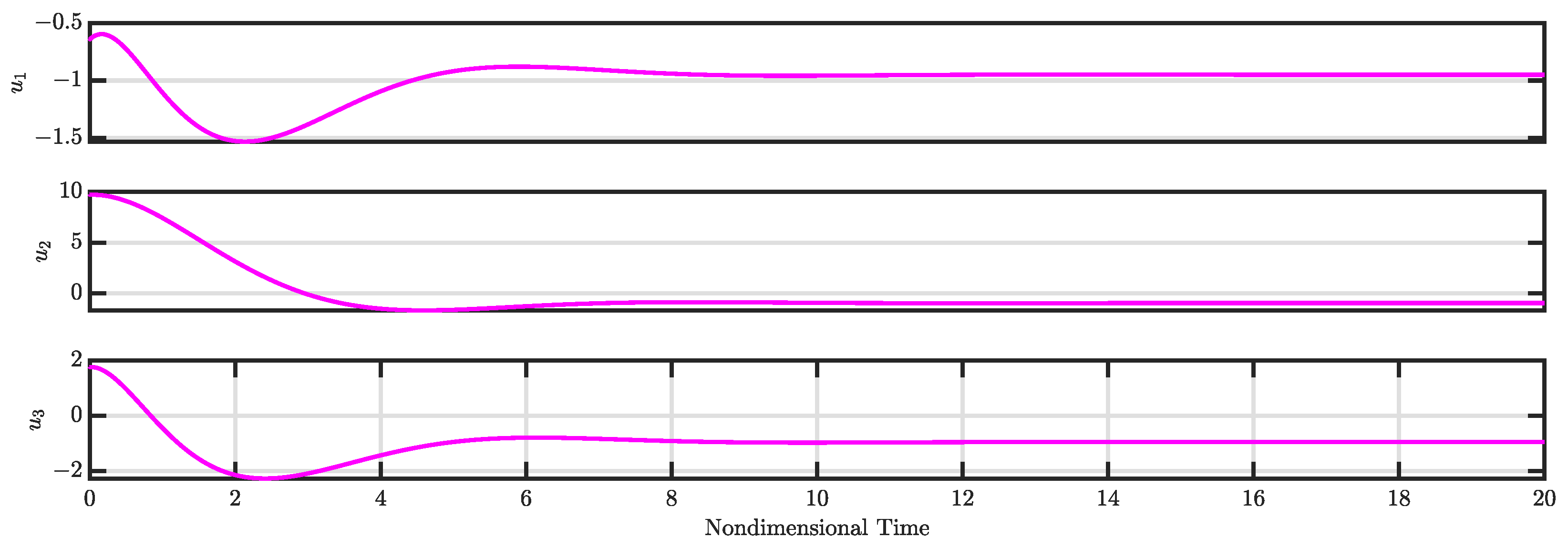
Figure 3 presents the time evolution of the modes ${\eta }_1\left(t\right)$ and ${\eta }_2\left(t\right)$ under closed-loop controller operation, while Figure 4 displays the commanded control signals.

Throughout the closed-loop operation, the control actuation stays within acceptable limits. The results clearly demonstrate the effectiveness of the proposed robust nonlinear control law in driving the states to zero.

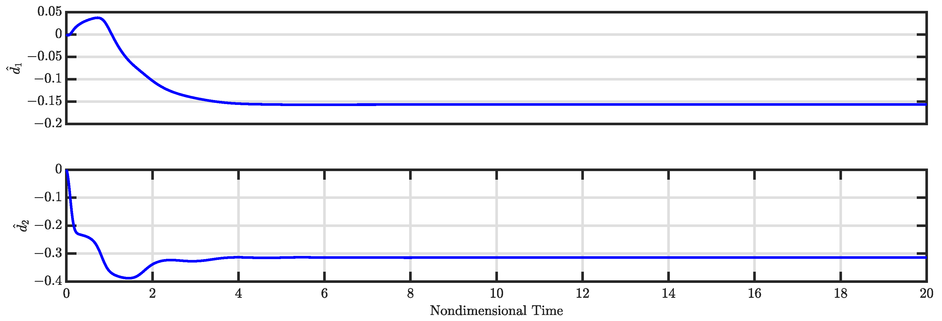
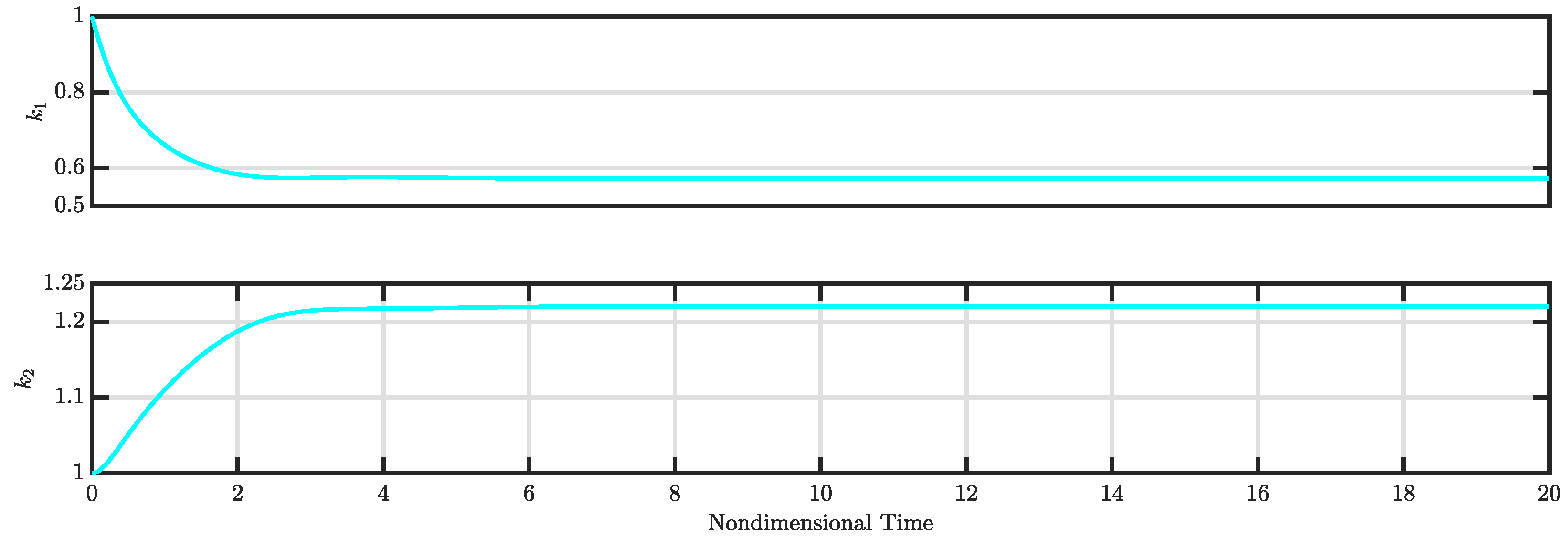
The calculated control gains (i.e., $k_1$ and $k_2$) along with the estimated disturbances (i.e., ${\widehat{d}}_1$ and ${\widehat{d}}_2$) for the controlled system are illustrated in Figure 5 and Figure 6, respectively. Figure 5 indicates that both control gains $k_1$ and $k_2$ converge to specific values, leading to a stable controlled system. Meanwhile, Figure 6 demonstrates that the estimated disturbances are effectively compensated, highlighting the capability of the nonlinear controller to estimate and mitigate these disturbances.

3.2. Case 2

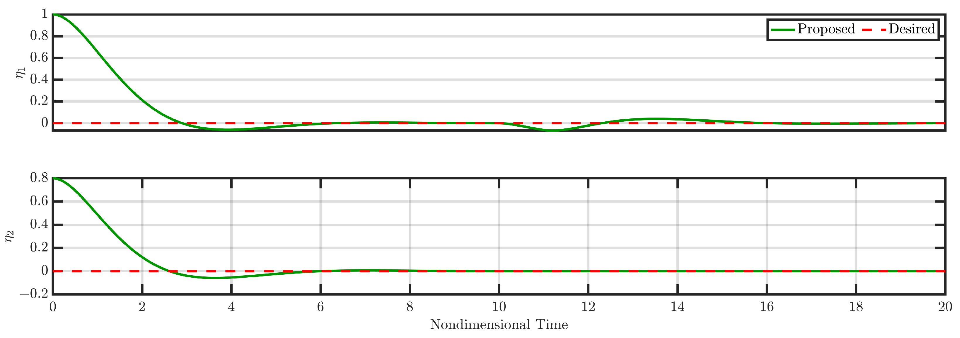
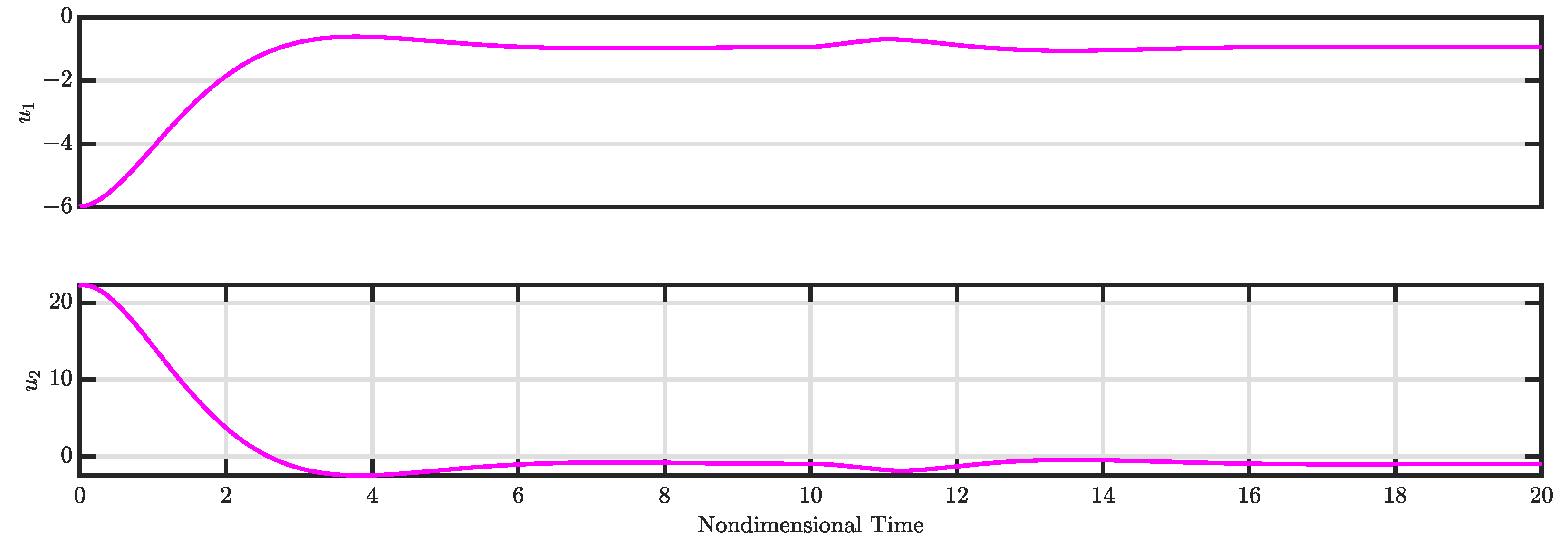
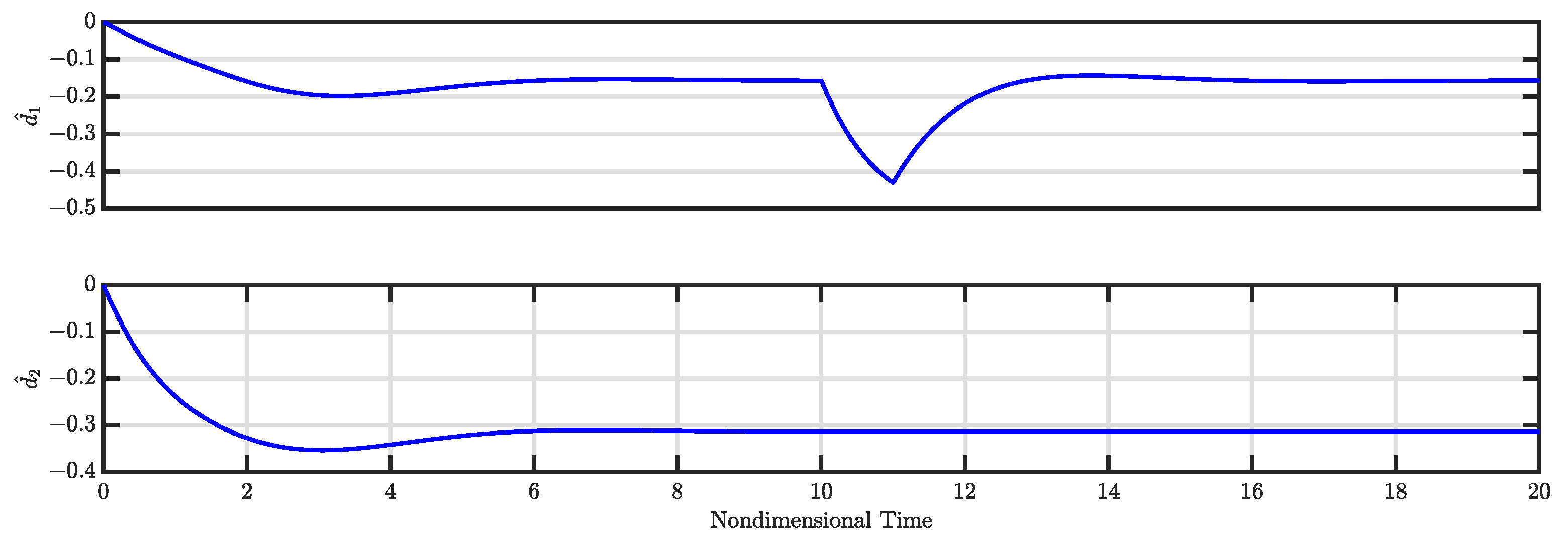
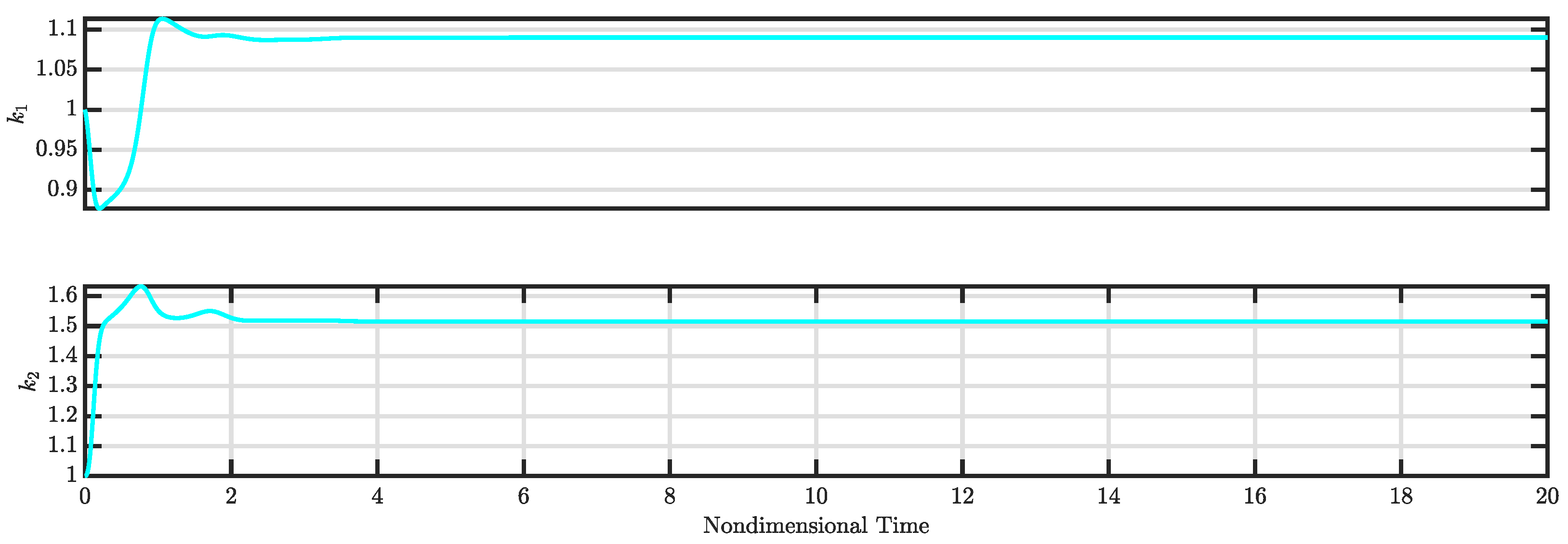
To study the robustness of the developed controller under large external disturbances, we applied an external large disturbance in the range of [10–11] seconds. The results of simulation for the closed loop are depicted in Figure 7 and Figure 8.

Figure 7 presents the time evolution of the modes ${\eta }_1\left(t\right)$ and ${\eta }_2\left(t\right)$ under closed-loop controller operation, while Figure 8 displays the commanded control signals.

Throughout the closed-loop operation, the control actuation stays within acceptable limits. The results clearly demonstrate the effectiveness of the proposed robust nonlinear control law in driving the states to zero.

The calculated control gains (i.e., $k_1$ and $k_2$) along with the estimated disturbances (i.e., ${\widehat{d}}_1$ and ${\widehat{d}}_2$) for the controlled system are illustrated in Figure 9 and Figure 10, respectively. Figure 9 indicates that both control gains $k_1$ and $k_2$ converge to specific values, leading to a stable controlled system. Meanwhile, Figure 10 demonstrates that the estimated disturbances are effectively compensated, highlighting the capability of the nonlinear controller to estimate and mitigate these disturbances.

3.3. Case 3

To study the robustness of the developed controller under system uncertainties (e.g., modeling errors, etc.), in our controller design for this case, we considered the system matrix $\widehat{M}=M\pm \%25$, which would result in the other two system matrices (i.e., C and G) being uncertain as well. The results of simulation for the closed loop are depicted in Figure 11 and Figure 12.

Figure 11 presents the time evolution of the modes ${\eta }_1\left(t\right)$ and ${\eta }_2\left(t\right)$ under closed-loop controller operation, while Figure 12 displays the commanded control signals.

Throughout the closed-loop operation, the control actuation stays within acceptable limits. The results clearly demonstrate the effectiveness of the proposed robust nonlinear control law in driving the states to zero.

The calculated control gains (i.e., $k_1$ and $k_2$) along with the estimated disturbances (i.e., ${\widehat{d}}_1$ and ${\widehat{d}}_2$) for the controlled system are illustrated in Figure 13 and Figure 14, respectively. Figure 13 indicates that both control gains $k_1$ and $k_2$ converge to specific values, leading to a stable controlled system. Meanwhile, Figure 14 demonstrates that the estimated disturbances are effectively compensated, highlighting the capability of the nonlinear controller to estimate and mitigate these disturbances.

3.4. Case 4

To study the scalability of the developed controller to higher-order systems, we considered the number of modes and actuators to both be three (i.e., $N=K=3$). The results of simulation for the closed loop are depicted in Figure 15 and Figure 16.

Figure 15 presents the time evolution of modes ${\eta }_1\left(t\right)$, ${\eta }_2\left(t\right)$, and ${\eta }_3\left(t\right)$ under closed-loop controller operation, while Figure 16 displays the commanded control signals.

Throughout the closed-loop operation, the control actuation stays within acceptable limits. The results clearly demonstrate the effectiveness of the proposed robust nonlinear control law in driving the states to zero.

The calculated control gains (i.e., $k_1$ and $k_2$) along with the estimated disturbances (i.e., ${\widehat{d}}_1$, ${\widehat{d}}_2$, and ${\widehat{d}}_3$) for the controlled system are illustrated in Figure 17 and Figure 18, respectively. Figure 17 indicates that both control gains $k_1$ and $k_2$ converge to specific values, leading to a stable controlled system. Meanwhile, Figure 18 demonstrates that the estimated disturbances are effectively compensated, highlighting the capability of the nonlinear controller to estimate and mitigate these disturbances.

4. Conclusions

This paper presents a robust controller based on simple learning techniques, designed to asymptotically stabilize thermoacoustic oscillations in a Rijke-type system amidst unknown disturbances and model uncertainties. The model is initially framed in a standard nonlinear control system format. A robust nonlinear controller has been developed to address the unmodeled nonlinearities and disturbances. The effectiveness of the nonlinear controller is demonstrated, achieving asymptotic stabilization of an uncertain multi-mode thermoacoustic system. The computer simulation results showcase the proposed control law’s effectiveness.

References

1. Kim, K.T.; Hochgreb, S. Measurements of triggering and transient growth in a model lean-premixed gas turbine combustor. Combust. Flame 2012, 159, 1215–1227. [Google Scholar] [CrossRef]
2. Lazik, W.; Doerr, T.; Bake, S.; vd Bank, R.; Rackwitz, L. Development of lean-burn low-NOx combustion technology at Rolls-Royce Deutschland. In Proceedings of the Turbo Expo: Power for Land, Sea, and Air, Berlin, Germany, 9–13 June 2008; Volume 43130, pp. 797–807. [Google Scholar]
3. Semlitsch, B.; Hynes, T.; Langella, I.; Swaminathan, N.; Dowling, A.P. Entropy and vorticity wave generation in realistic gas turbine combustors. J. Propuls. Power 2019, 35, 839–849. [Google Scholar] [CrossRef]
4. Richards, G.A.; Straub, D.L.; Robey, E.H. Passive control of combustion dynamics in stationary gas turbines. J. Propuls. Power 2003, 19, 795–810. [Google Scholar] [CrossRef]
5. Gysling, D.L.; Copeland, G.S.; McCormick, D.C.; Proscia, W.M. Combustion system damping augmentation with Helmholtz resonator. J. Eng. Gas Turbines Power 2000, 122, 269–274. [Google Scholar] [CrossRef]
6. Zhao, D.; Morgans, A.S. Tuned passive control of combustion instabilities using multiple Helmholtz resonators. J. Sound Vib. 2009, 320, 744–757. [Google Scholar] [CrossRef]
7. Eldredge, J.D.; Dowling, A.P. The absorption of axial acoustic wave by a perforated liner with bias flow. J. Fluid Mech. 2003, 485, 307–335. [Google Scholar] [CrossRef]
8. Zhong, Z.; Zhao, D. Time-domain characterizaton of the acoustic damping of a perforated liner with bias flow. J. Acoust. Soc. Am. 2012, 132, 271–281. [Google Scholar] [CrossRef]
9. McManus, K.; Poinsot, T.; Candel, S.M. A review of active control of combustion instabilities. Prog. Energy Combust. Sci. 1993, 19, 1–29. [Google Scholar] [CrossRef]
10. Dowling, A.P.; Morgans, A.S. Feedback control of combustion oscillations. Annu. Rev. Fluid Mech. 2005, 37, 151–182. [Google Scholar] [CrossRef]
11. Olgac, N.; Zalluhoglu, U.; Kammer, A.S. A new perspective in designing delayed feedback control for thermoacoustic instabilities (TAI). Combust. Sci. Technol. 2015, 187, 697–720. [Google Scholar] [CrossRef]
12. Heckl, M.A. Active control of the noise from a Rijke tube. J. Sound Vib. 1988, 124, 117–133. [Google Scholar] [CrossRef]
13. Zhao, D.; Chow, Z. Thermoacoustic instability of a laminar premixed flame in Rijke tube with a hydrodynamic region. J. Sound Vib. 2013, 332, 3419–3437. [Google Scholar] [CrossRef]
14. Seume, J.; Vortmeyer, N.; Krause, W.; Hermann, J.; Hantschk, C.C.; Zangl, P.; Gleis, S.; Vortmeyer, D.; Orthmann, A. Application of active combustion instability control to a heavy duty gas turbine. J. Eng. Gas Turbines Power 1998, 120, 721–726. [Google Scholar] [CrossRef]
15. Sattinger, S.S.; Neumeier, Y.; Nabi, A.; Zinn, B.T.; Amos, D.J.; Darling, D.D. Sub-scale demonstration of the active feedback control of gas turbine combustion instability. Trans. ASME 2000, 262, 262–268. [Google Scholar] [CrossRef]
16. Mondal, S.; Chattopadhyay, A.; Mukhopadhyay, A.; Ray, A. Transfer learning of deep neural networks for predicting thermoacoustic instabilities in combustion systems. Energy AI 2021, 5, 10085. [Google Scholar] [CrossRef]
17. Xie, M.; Zhao, X.; Zhao, D.; Fu, J.; Shelton, C.; Semlitsch, B. Predicting bifurcation and amplitude death characteristics of thermoacoustic instabilities from PINNs-derived van der Pol oscillators. J. Fluid Mech. 2024, 998, A46. [Google Scholar] [CrossRef]
18. Zhao, D.; Lu, Z.; Ahao, H.; Li, X.Y.; Wang, B.; Liu, P. A review of active control approaches in stabilizing combustion systems in aerospace industry. Prog. Aerosp. Sci. 2018, 97, 35–60. [Google Scholar] [CrossRef]
19. Campos-Delgado, D.U.; Zhou, K.; Allgood, D.; Acharya, S. Active control of combustion instabilities using model-based controllers. Combust. Sci. Technol. 2003, 175, 27–53. [Google Scholar] [CrossRef]
20. Annaswamy, A.M.; Fleifil, M.; Hathout, J.P.; Ghoniem, A.F. Impact of linear coupling on the design of active controllers for thermoacoustic instability. Combust. Sci. Technol. 1997, 128, 131–180. [Google Scholar] [CrossRef]
21. Hervas, J.R.; Zhao, D.; Reyhanoglu, M. Nonlinear feedback control of self-sustained thermoacoustic oscillations. Aerosp. Sci. Technol. 2015, 41, 209–215. [Google Scholar] [CrossRef]
22. Hervas, J.R.; Reyhanoglu, M.; MacKunis, W. Sliding mode control of Rijke-type thermoacoustic systems. In Proceedings of the IEEE Workshop on Recent Advances in Sliding Modes (RASM), Istanbul, Turkey, 9–11 April 2015; pp. 1–6. [Google Scholar]
23. Edwards, C.; Spurgeon, S.K. Sliding Mode Control. Theory and Applications; Taylor and Francis: Abingdon, Thames, UK, 1998. [Google Scholar]
24. Kayacan, E. Sliding mode learning control of uncertain nonlinear systems with Lyapunov stability analysis. Trans. Inst. Meas. Control 2019, 41, 1750–1760. [Google Scholar] [CrossRef]
25. Topalov, A.V.; Kaynak, O. Online learning in adaptive neurocontrol schemes with a sliding mode algorithm. IEEE Trans. Syst. Man, Cybern. Part B (Cybern.) 2001, 31, 445–450. [Google Scholar] [CrossRef] [PubMed]
26. Kayacan, E.; Kayacan, E.; Ramon, H.; Saeys, W. Learning in centralized nonlinear model predictive control: Application to an autonomous tractor-trailer system. IEEE Trans. Control Syst. Technol. 2014, 23, 197–205. [Google Scholar] [CrossRef]
27. Kocer, B.B.; Tjahjowidodo, T.; Seet, G.G.L. Centralized predictive ceiling interaction control of quadrotor VTOL UAV. Aerosp. Sci. Technol. 2018, 76, 455–465. [Google Scholar] [CrossRef]
28. Fu, C.; Hong, W.; Lu, H.; Zhang, L.; Guo, X.; Tian, Y. Adaptive robust backstepping attitude control for a multi-rotor unmanned aerial vehicle with time-varying output constraints. Aerosp. Sci. Technol. 2018, 78, 593–603. [Google Scholar] [CrossRef]
29. Wu, B.; Wu, J.; He, W.; Tang, G.; Zhao, Z. Adaptive neural control for an uncertain 2-DOF helicopter system with unknown control direction and actuator faults. Mathematics 2022, 10, 4342. [Google Scholar] [CrossRef]
30. Xu, Z.; Li, W.; Wang, Y. Robust learning control for shipborne manipulator with fuzzy neural network. Front. Neurorobotics 2019, 13, 11. [Google Scholar] [CrossRef] [PubMed]
31. Kayacan, E.; Fossen, T.I. Feedback linearization control for systems with mismatched uncertainties via disturbance observers. Asian J. Control 2019, 21, 1064–1076. [Google Scholar] [CrossRef]
32. Şahin, S. Learning feedback linearization using artificial neural networks. Neural Process. Lett. 2016, 44, 625–637. [Google Scholar] [CrossRef]
33. Chi, R.; Hou, Z.; Huang, B.; Jin, S. A unified data-driven design framework of optimality-based generalized iterative learning control. Comput. Chem. Eng. 2015, 77, 10–23. [Google Scholar] [CrossRef]
34. You, S.; Son, Y.S.; Gui, Y.; Kim, W. Gradient-descent-based learning gain for backstepping controller and disturbance observer of nonlinear systems. IEEE Access 2023, 11, 2743–2753. [Google Scholar] [CrossRef]
35. Reyhanoglu, M.; Jafari, M. A simple learning approach for robust tracking control of a class of dynamical systems. Electronics 2023, 12, 2026. [Google Scholar] [CrossRef]
36. Jafari, M.; Reyhanoglu, M.; Kozhabek, Z. Simple learning-based robust nonlinear control of an electric pump for liquid-propellant rocket engines. Electronics 2023, 12, 3527. [Google Scholar] [CrossRef]
37. Reyhanoglu, M.; Jafari, M.; Rehan, M. Simple learning-based robust trajectory tracking control of a 2-DOF helicopter system. Electronics 2022, 11, 2075. [Google Scholar] [CrossRef]
38. Hajiahmadi, F.; Jafari, M.; Reyhanoglu, M. Machine learning-based control of autonomous vehicles for solar panel cleaning systems in agricultural solar farms. AgriEngineering 2024, 6, 1417–1435. [Google Scholar] [CrossRef]
39. Epperlein, J.P.; Bamieh, B.; Astrom, K.J. Thermoacoustics and the Rijke tube: Experiments, identification, and modeling. IEEE Control Syst. Mag. 2015, 35, 57–77. [Google Scholar]
40. Fleifil, M.; Hathout, J.P.; Annaswamy, A.M.; Ghoniem, A.F. The origin of secondary peaks with active control of thermoacoustic instability. Combust. Sci. Technol. 1998, 133, 227–265. [Google Scholar] [CrossRef]
41. Juniper, M.P. Triggering in the horizontal rijke tube: Non-normality, transient growth and bypass transition. J. Fluid Mech. 2011, 667, 272–308. [Google Scholar] [CrossRef]
42. Matveev, K.I.; Culick, F.C. A model for combustion instability involving vortex shedding. Combust. Sci. Technol. 2003, 185, 1059–1083. [Google Scholar] [CrossRef]
Figure 1. A depiction of the thermoacoustic system.
Electronics 14 01771 g001
Figure 2. Responses of η 1 and η 2 (open loop). Dashed red line shows the zero line and the solid green line shows the system’s open-loop response.
Electronics 14 01771 g002
Figure 3. Responses of η 1 and η 2 (closed loop) for Case 1 (see Section 3.1).
Electronics 14 01771 g003
Figure 4. Control inputs u 1 and u 2 for Case 1 (see Section 3.1).
Electronics 14 01771 g004
Figure 5. k 1 and k 2 for Case 1 (see Section 3.1).
Electronics 14 01771 g005
Figure 6. d 1 ^ and d 2 ^ for Case 1 (see Section 3.1).
Electronics 14 01771 g006
Figure 7. Responses of η 1 and η 2 (closed loop) for Case 2 (see Section 3.2).
Electronics 14 01771 g007
Figure 8. Control inputs u 1 and u 2 for Case 2 (see Section 3.2).
Electronics 14 01771 g008
Figure 9. k 1 and k 2 for Case 2 (see Section 3.2).
Electronics 14 01771 g009
Figure 10. d 1 ^ and d 2 ^ for Case 2 (see Section 3.2).
Electronics 14 01771 g010
Figure 11. Responses of η 1 and η 2 (closed loop) for Case 3 (see Section 3.3).
Electronics 14 01771 g011
Figure 12. Control inputs u 1 and u 2 for Case 3 (see Section 3.3).
Electronics 14 01771 g012
Figure 13. k 1 and k 2 for Case 3 (see Section 3.3).
Electronics 14 01771 g013
Figure 14. d 1 ^ and d 2 ^ for Case 3 (see Section 3.3).
Electronics 14 01771 g014
Figure 15. Responses of η 1 , η 2 , and η 3 (closed loop) for Case 4 (see Section 3.4).
Electronics 14 01771 g015
Figure 16. Control inputs u 1 , u 2 , and u 3 for Case 4 (see Section 3.4).
Electronics 14 01771 g016
Figure 17. k 1 and k 2 for Case 4 (see Section 3.4).
Electronics 14 01771 g017
Figure 18. d 1 ^ , d 2 ^ , and d 3 ^ for Case 4 (see Section 3.4).
Electronics 14 01771 g018