


Research on Distributed Smart Home Energy Management Strategies Based on Non-Intrusive Load Monitoring (NILM)

Abstract
1. Introduction
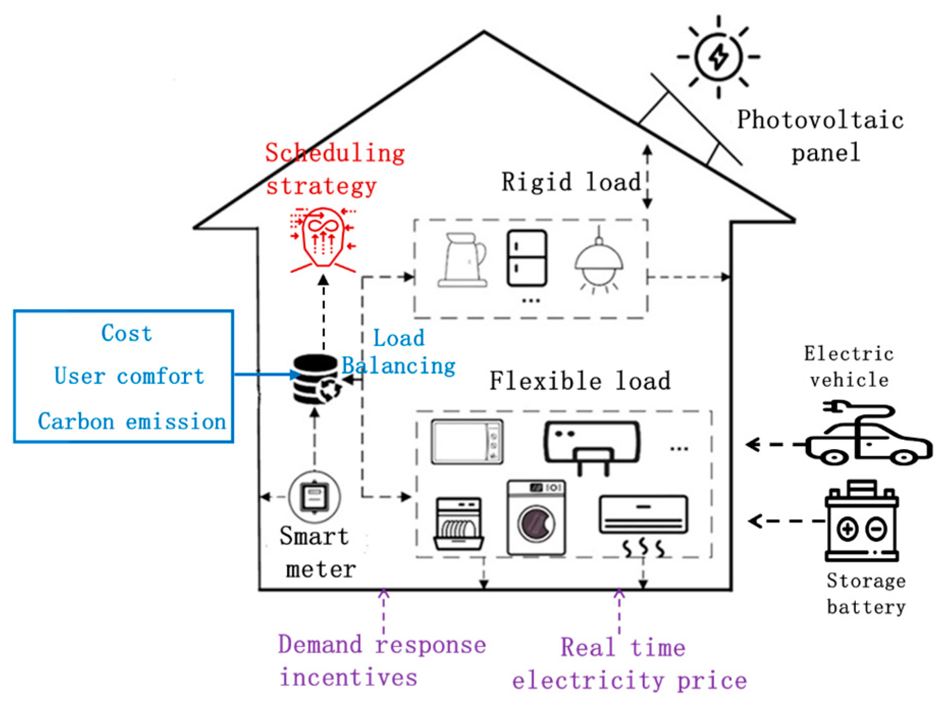
2. Smart Home Energy Management
2.1. Home Energy Management
2.2. Household Load Model
- Power-adjustable load: These loads have adjustable power output through step control, such as air conditioners, water heaters, and lighting. The energy consumption of these devices can be controlled by adjusting their power levels. The model is expressed as
- Time-adjustable load: These loads, such as washing machines and dishwashers, can have their operating times adjusted. Once started, they must complete their entire work cycle without interruption. The model is
- Power-time adjustable load: Power-time loads are time-variable and interruptible loads, such as electric vehicles and other new energy transportation tools. Due to their flexible adjustability, they are a primary target for demand-side response scheduling. In a sense, they can be considered a form of energy storage without the discharge process. Power-time loads can be modeled using a power-time function, where both the power and time of operation are adjustable and can be interrupted within a certain time period. Charging an electric vehicle or a battery is a common example, where the charging power can be adjusted or interrupted during a time period, and the charging process is considered a variable time window. The model can be expressed as follows:
- Temperature-controlled adjustable load: These are loads whose operation is influenced by temperature constraints, with their operating status depending on indoor and outdoor temperatures, set temperature values, and the thermal properties of the building. The indoor temperature setting is determined based on user demand within a given time period. When required, the indoor temperature should remain within the upper and lower bounds of the specified value. The mathematical model for air conditioners and water heaters is typically represented by a discrete thermal dynamic model as shown:
2.3. DR Incentives
- Time-of-Use Pricing
- DR Compensation
2.4. User Comfort
- Time Comfort
- Temperature Comfort
2.5. Carbon Emissions and Carbon Consumption
2.6. Load Balancing
- 1.
- Let represent the system load at the -th moment and represent the average system load over time periods. The system load dispersion can be defined as the standard deviation of the system load.
- 2.
- The baseline flatness calculation is calculated as
- 3.
- Let represent the flexible load in the -th period. The correlation or matching degree between the control variable and system load fluctuations can be calculated as
- 4.
- Finally, the flatness index can be calculated as
3. SHEM Based on Mixed-Integer Linear Programming
3.1. Objective Function
3.2. Calculation of Efficacy Coefficients
- (1)
- For the economic optimization objective Z, T, , the calculation method for its efficacy coefficient is
- (2)
- For the comfort optimization objective , which consists of time comfort and temperature comfort, the efficiency coefficient calculation method is
- (3)
- The calculation method for the efficiency coefficient of the flatness optimization objective H is
3.3. Mixed-Integer Linear Programming
- Branching: The original problem is decomposed into several subproblems (subnodes); each subproblem reduces the solution space by adding additional constraints (e.g., fixing the integer values of variables).
- Bounding: By solving the relaxed version of the subproblem (e.g., linear programming relaxation), upper and lower bounds are calculated. These bounds are used to prune branches that cannot contain the optimal solution, thereby reducing the computational effort.
- Create the root node corresponding to the original MILP problem.
- Set the global upper bound (UB) and the lower bound (LB).
- Perform linear programming relaxation on the current node (ignoring integer constraints) to solve the relaxed problem:
- If the relaxed problem has no feasible solution, prune this branch; otherwise, obtain the relaxed solution and its objective value .
- Optimality Pruning: If the relaxed solution satisfies the integer constraints, update the global upper bound as min (,UB) and record this solution.
- Bounding Pruning: If ≥ UB, it means that this branch cannot produce a better solution, so prune this branch. Otherwise, update LB = max ().
- Subproblem 1:
- Subproblem 2:
- Use depth-first search (DFS) to select the next node to process from the queue. DFS is a tree/graph traversal or search strategy that prioritizes exploring along one branch as deeply as possible until a leaf node is reached or no further progress is possible. In branch and bound, DFS processes the most recently generated subnodes first, quickly delving deeper into the tree, potentially finding feasible solutions early, which can update the global upper bound and trigger pruning, thus reducing the exploration of subsequent invalid branches.
- All branches have been pruned or processed.
- The difference between the global UB and LB is smaller than the preset threshold ϵ = 10−4.
3.4. Hybrid Genetic Branch-and-Bound Algorithm
- Encode the integer variables of MILP into gene sequences.
- Randomly generate O individuals (O = 50), calculate the fitness value of each individual, and record the optimal solution .
- Let the global upper bound be the initial optimal solution UB = and the lower bound LB = .
- Add the original MILP problem as the root node to the active node queue, and prioritize the queue by LP relaxation value.
- Perform linear programming relaxation on the current node (ignoring integer constraints) to solve the relaxed problem.
- If the relaxed problem has no feasible solution, prune this branch; otherwise, obtain the relaxed solution and its objective value .
- Optimality Pruning: If the relaxed solution satisfies the integer constraints, update the global upper bound as min (,UB), and record this solution.
- Bounding Pruning: If ≥ UB, it means that this branch cannot produce a better solution, so prune this branch. Otherwise, update LB = max ().
- Subproblem 1:
- Subproblem 2:
- Trigger Conditions:
- Process K = 50 branch and bound nodes;
- No update to the global UB for T = 10 consecutive iterations;
- LP relaxation solution is close to integrality (e.g., fractional variables have values near 0 or 1).
- Genetic Operations:
- Crossover: Combine the current best solution xi with the rounded integer solution to round() to generate offspring.
- Mutation: Apply random perturbations (e.g., flipping binary variables or adjusting integer values) to offspring while ensuring constraint satisfaction.
- Selection: Retain the top p = 20 individuals with the highest fitness (i.e., lowest objective value f(x)).
- Update Upper Bound:
- Dynamic Pruning:
- All branches have been pruned or processed.
- The difference between the global UB and LB is smaller than the preset threshold ϵ = 10−4.
3.5. Constraints
3.5.1. Balance Constraints
3.5.2. Load Operation Constraints
- Operating Time Range: The device must start within the allowed operating time window, for example, prioritizing operation during off-peak hours with lower electricity rates.
- Optimal Comfort Time Window: The load should operate primarily within the user’s desired time window, such as having the dishwasher automatically run after dinner.
- Minimum/Maximum Power Limits:
- Minimum/Maximum Capacity Limits:
- Load Distribution Balance: These loads should operate primarily during periods with low electricity rates and low grid load to flatten the peak demand and fill the valley periods.
- Temperature range for adjustment: For air conditioning, the cooling temperature cannot fall below a set lower limit, and in heating mode, it cannot exceed a set upper limit. For water heaters, the minimum water temperature must meet household needs.
- Optimal temperature comfort range: The temperature should ideally be maintained within the user’s most comfortable range, such as keeping air conditioning between 24–26 °C and water heaters between 45–55 °C, balancing both comfort and energy efficiency.
- Dynamic adjustment mechanism: The system adjusts the operation strategy based on environmental temperature, load status, and electricity prices. For example, the air conditioning temperature setpoint can be raised during peak times to reduce energy consumption.
4. Example Analysis
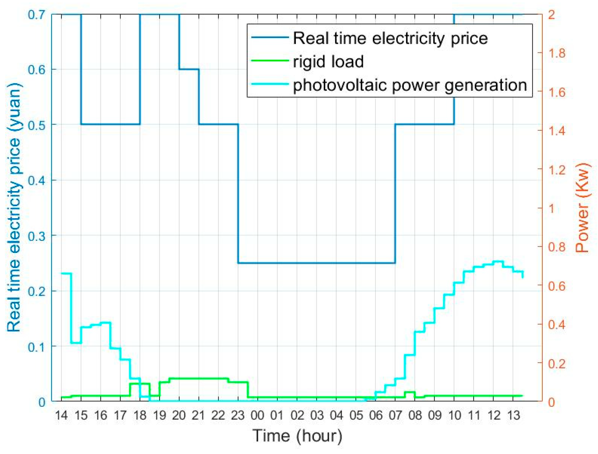
4.1. Parameter Settings
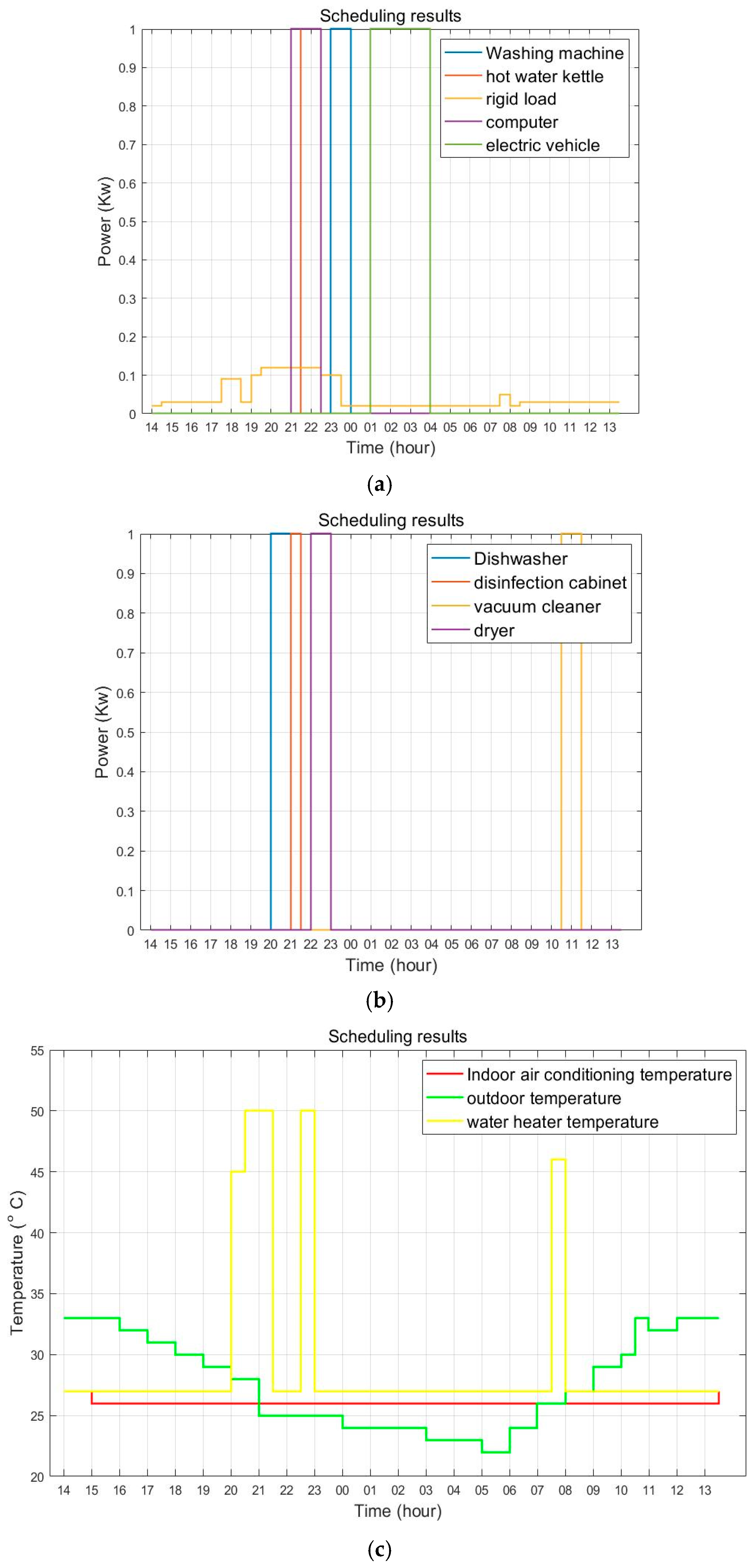
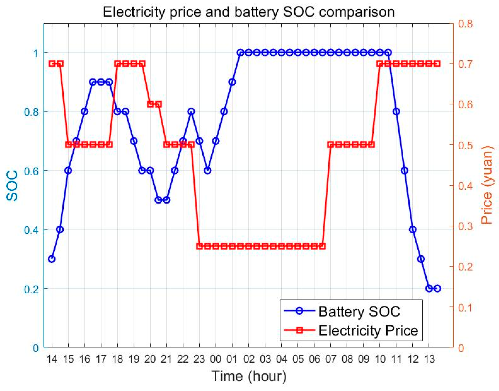
4.2. Simulation and Result Analysis
- Scenario 1: Only electricity cost is considered, while user comfort is not taken into account.
- Scenario 2: A comprehensive consideration of electricity cost, user comfort, load curve flatness, and carbon consumption.
5. Conclusions
Author Contributions
Funding
Data Availability Statement
Conflicts of Interest
References
- Mischos, S.; Dalagdi, E.; Vrakas, D. Intelligent energy management systems: A review. Artif. Intell. Rev. 2023, 56, 11635–11674. [Google Scholar] [CrossRef]
- Li, J.; Zhou, Z. Distributed energy management and optimization analysis in smart grids. Electron. Technol. 2024, 53, 286–287. [Google Scholar]
- Ajao, A.; Luo, J.; Liang, Z.; Alsafasfeh, Q.H.; Su, W. Intelligent home energy management system for distributed renewable generators, dispatchable residential loads, and distributed energy storage devices. In Proceedings of the 8th International Renewable Energy Congress (IREC), Amman, Jordan, 21–23 March 2017; pp. 1–6. [Google Scholar] [CrossRef]
- Kwon, K.; Lee, S.; Kim, S. AI-Based Home Energy Management System Considering Energy Efficiency and Resident Satisfaction. IEEE Internet Things J. 2022, 9, 1608–1621. [Google Scholar] [CrossRef]
- Yang, Q.; Wang, H. Privacy-Preserving Transactive Energy Management for IoT-Aided Smart Homes via Blockchain. arXiv 2021, arXiv:2101.03840. [Google Scholar] [CrossRef]
- Dong, X.; Shao, X.; Guan, R. Cost optimization problem of home energy management system based on particle swarm algorithm. Comput. Knowl. Technol. 2021, 17, 122–124. [Google Scholar] [CrossRef]
- Ruan, B.J. Energy Optimization Scheduling Method for Home Hybrid Power Supply System Considering Real-Time Electricity Prices. Ph.D. Thesis, Zhejiang University, Hangzhou, China, 2015. [Google Scholar]
- Yin, Z.D.; Lin, Z.; Li, D.Z. Intelligent home energy management strategy based on hybrid particle swarm optimization algorithm. J. North China Electr. Power Univ. (Nat. Sci. Ed.) 2018, 45, 25–33. [Google Scholar]
- Zhang, T.; Zhao, Q.; Chen, Z.; Wang, R.; Xing, Q.; Tian, J. Hierarchical optimization strategy for home energy management based on deep reinforcement learning. Autom. Electr. Power Syst. 2021, 45, 149–158. [Google Scholar]
- Zhang, K.J.; Ding, G.F.; Wen, M.; Hui, H.; Ding, Y.; He, M. Optimization scheduling technology and market mechanism design of virtual power plants: A review. Compr. Smart Energy 2022, 44, 60–72. [Google Scholar]
- Wei, G.; Chi, M.; Liu, Z.W.; Ge, M.; Li, C.; Liu, X. Deep reinforcement learning for real-time energy management in smart home. IEEE Syst. J. 2023, 17, 2489–2499. [Google Scholar] [CrossRef]
- Ye, Y.J.; Wang, H.Y.; Tang, Y. Optimal autonomous energy management strategy for residents based on deep reinforcement learning. Autom. Electr. Power Syst. 2022, 46, 110–119. [Google Scholar]
- Ma, Y.; Chen, X.; Wang, L.; Yang, J. Study on smart home energy management system based on artificial intelligence. J. Sens. 2021, 2021, 9101453. [Google Scholar] [CrossRef]
- Navesi, R.B.; Naghibi, A.F.; Zafarani, H.; Tahami, H.; Pirouzi, S. Reliable operation of reconfigurable smart distribution network with real-time pricing-based demand response. Electr. Power Syst. Res. 2025, 241, 111341. [Google Scholar] [CrossRef]
- Hu, R.; Zhou, K.; Yin, H. Reinforcement learning model for incentive-based integrated demand response considering demand-side coupling. Energy 2024, 308, 132997. [Google Scholar] [CrossRef]
- Dey, B.; Sharma, G.; Bokoro, P.N.; Dutta, S. An intelligent incentive-based demand response program for exhaustive environment-constrained techno-economic analysis of microgrid systems. Sci. Rep. 2025, 15, 894. [Google Scholar] [CrossRef] [PubMed]
- Ikram, A.I.; Ullah, A.; Datta, D.; Islam, A.; Ahmed, T. Optimizing energy consumption in smart homes: Load scheduling approaches. IET Power Electron. 2024, 17, 2656–2668. [Google Scholar] [CrossRef]
- Akram, A.; Abbas, S.; Khan, M.; Athar, A.; Ghazal, T.; Al Hamadi, H. Smart energy management system using machine learning. Comput. Mater. Contin. 2024, 78, 959–973. [Google Scholar] [CrossRef]
- Youssef, H.; Kamel, S.; Hassan, M.H.; Yu, J.; Safaraliev, M. A smart home energy management approach incorporating an enhanced northern goshawk optimizer to enhance user comfort, minimize costs, and promote efficient energy consumption. Int. J. Hydrogen Energy 2024, 49, 644–658. [Google Scholar] [CrossRef]
- Youssef, H.; Kamel, S.; Hassan, M.H.; Nasrat, L.; Jurado, F. An improved bald eagle search optimization algorithm for optimal home energy management systems. Soft Comput. 2024, 28, 1367–1390. [Google Scholar] [CrossRef]
- Wu, H.C.; Wang, C.; Zuo, Y.L.; Chen, Y.J.; Liu, K. Home energy system optimization based on time-of-use pricing and real-time control strategy for batteries. Power Syst. Prot. Control. 2019, 47, 23–30. [Google Scholar] [CrossRef]
- Yang, Y. A review of the carbon emission factor method’s application to power system accounting. Appl. Comput. Eng. 2023, 26, 120–125. [Google Scholar] [CrossRef]

| Abbreviations | Meanings |
|---|---|
| SHEM | Smart home energy management |
| NILM | Non-intrusive load monitoring |
| AI | Artificial intelligence |
| IoT | Internet of Things |
| MILP | Mixed-integer linear programming |
| GA | Genetic algorithm |
| DR | Demand response |
| Time-of-use pricing | |
| State of charge | |
| Photovoltaic | |
| RTP | Real-time pricing |
| EV | Electric vehicle |
| B&B | Branch and bound |
| LP | Linear programming |
| MDP | Markov decision process |
| LSTM | Long short-term memory |
| HVAC | Heating, ventilation, and air conditioning |
| CNY | Chinese yuan |
| Appliance Name | Power (kW) | Operating Window | Required Operating Duration (h) | Minimum Continuous Operating Duration (h) |
|---|---|---|---|---|
| Washing Machine | 0.5 | 12:00–22:00 | 1 | 1 |
| Kettle | 1.5 | 18:00–07:00 | 0.5 | 0.5 |
| Vacuum Cleaner | 1.0 | 08:00–12:00 | 1 | 1 |
| Dishwasher | 0.5 | 19:00–02:00 | 1 | 1 |
| Disinfection Cabinet | 0.3 | 19:00–07:00 | 0.5 | 0.5 |
| Tumble Dryer | 1.5 | 19:00–07:00 | 1 | 1 |
| Electric Car | 3.0 | 18:00–06:00 | 3 | 1 |
| Computer | 0.15 | 19:00–24:00 | 1.5 | 1 |
| Air Conditioner | 2.0 | All day | - | - |
| Water Heater | 2.5 | 07:00–00:00 | - | - |
| Symbols | Meanings |
|---|---|
| Prigid (t) | Power of the rigid load at time t |
| Prated(t) | Rated power of the load at time t |
| Padjustable (t) | Power-adjustable load |
| Pflexible (t) | Power-time adjustable load |
| SOC (t) | State of charge of the battery at time t |
| Time comfort of device i at time t | |
| Temperature comfort of device i at time t | |
| Carbon emission factor | |
| Electricity cost of the load excluding photovoltaic output | |
| Electricity price at time t | |
| Photovoltaic power generation | |
| Quantified flatness of the net load curve | |
| Total incentive subsidy from demand response | |
| Total carbon emission cost for one period | |
| Carbon emissions (or carbon consumption) at period t | |
| Room thermal capacity | |
| Relaxed solution | |
| UB | Upper bound |
| LB | Lower bound |
| DR | Demand response |
| Charging efficiencies | |
| Discharging efficiencies |
| Metrics | Methods of Efficacy Coefficients | Linear Weighting Method | ||
|---|---|---|---|---|
| Before Optimization | After Optimization | Before Optimization | After Optimization | |
| Flexible load electricity fee | 3.94 | 2.776 | 3.94 | 2.481 |
| Flatness of load curve | 1.23 | 1.84 | 1.23 | 1.46 |
| Carbon consumption | 1.418 | 0.994 | 1.418 | 0.883 |
| User comfort | 1 | 0.95 | 1 | 0.61 |
| Metrics | Scenario 1 | Scenario 2 | ||||
|---|---|---|---|---|---|---|
| GA | MILP | MILP +GA | GA | MILP | MILP +GA | |
| Flexible load electricity fee | 1.904 | 1.316 | 1.422 | 3.446 | 2.912 | 2.776 |
| Flatness of load curve | 1.049 | 1.274 | 1.315 | 1.54 | 1.71 | 1.84 |
| Carbon consumption | 0.669 | 0.571 | 0.476 | 1.214 | 1.133 | 0.994 |
| User comfort | 0.149 | 0.207 | 0.243 | 0.78 | 0.87 | 0.95 |
| Time (s) | 3346.8 | 139.74 | 3547.6 | 3538.1 | 141.54 | 3661.3 |
Disclaimer/Publisher’s Note: The statements, opinions and data contained in all publications are solely those of the individual author(s) and contributor(s) and not of MDPI and/or the editor(s). MDPI and/or the editor(s) disclaim responsibility for any injury to people or property resulting from any ideas, methods, instructions or products referred to in the content. |
© 2025 by the authors. Licensee MDPI, Basel, Switzerland. This article is an open access article distributed under the terms and conditions of the Creative Commons Attribution (CC BY) license (https://creativecommons.org/licenses/by/4.0/).
Share and Cite
Liu, S.; Xie, Z.; Hu, Z. Research on Distributed Smart Home Energy Management Strategies Based on Non-Intrusive Load Monitoring (NILM). Electronics 2025, 14, 1719. https://doi.org/10.3390/electronics14091719
Liu S, Xie Z, Hu Z. Research on Distributed Smart Home Energy Management Strategies Based on Non-Intrusive Load Monitoring (NILM). Electronics. 2025; 14(9):1719. https://doi.org/10.3390/electronics14091719
Chicago/Turabian StyleLiu, Siqi, Zhiyuan Xie, and Zhengwei Hu. 2025. "Research on Distributed Smart Home Energy Management Strategies Based on Non-Intrusive Load Monitoring (NILM)" Electronics 14, no. 9: 1719. https://doi.org/10.3390/electronics14091719
APA StyleLiu, S., Xie, Z., & Hu, Z. (2025). Research on Distributed Smart Home Energy Management Strategies Based on Non-Intrusive Load Monitoring (NILM). Electronics, 14(9), 1719. https://doi.org/10.3390/electronics14091719