Ultra-Lightweight and Highly Efficient Pruned Binarised Neural Networks for Intrusion Detection in In-Vehicle Networks

Abstract

With the rapid evolution toward autonomous vehicles, securing in-vehicle communications is more critical than ever. The widely used Controller Area Network (CAN) protocol lacks built-in security, leaving vehicles vulnerable to cyberattacks. Although machine learning-based Intrusion Detection Systems (IDSs) can achieve high detection accuracy, their heavy computational and power demands often limit real-world deployment. In this paper, we present an optimised IDS based on a Binarised Neural Network (BNN) that employs network pruning to eliminate redundant parameters, achieving up to a 91.07% reduction with only a 0.1% accuracy loss. The proposed approach incorporates a two-stage Coarse-to-Fine (C2F) framework, efficiently filtering normal traffic in the initial stage to minimise unnecessary processing. To assess its practical feasibility, we implement and compare the pruned IDS across CPU, GPU, and FPGA platforms. The experimental results indicate that, with the same model structure, the FPGA-based solution outperforms GPU and CPU implementations by up to 3.7× and 2.4× in speed, while achieving up to 7.4× and 3.8× greater energy efficiency, respectively. Among cutting-edge BNN-based IDSs, our ultra-lightweight FPGA-based C2F approach achieves the fastest average inference speed, showing a 3.3× to 12× improvement, while also outperforming them in accuracy and average F1 score, highlighting its potential for low-power, high-performance vehicle security.

1. Introduction

As vehicles evolve toward self-driving technology, security has become a growing concern. Modern vehicles rely on multiple sensors, actuators, and Electronic Control Units (ECUs) to enable intelligent features. Communication among ECUs is crucial to ensuring that each component operates synchronously. The Controller Area Network (CAN) is a common in-vehicle network due to its affordability, lightweight design, and resilience to noise. However, CAN lacks built-in security mechanisms, leaving it vulnerable to malicious nodes injecting unauthorised messages. Researchers have demonstrated that these vulnerabilities can be exploited via the On-Board Diagnostics (OBD-II) port [1] or through wireless communication systems [2,3]. Such attacks could mislead drivers with false information or even grant attackers control over critical vehicle functions, posing significant safety risks [4].

To enhance vehicle security, some studies have proposed adding a security layer to the CAN protocol, such as incorporating authentication [5,6] and encryption [7]. However, these methods introduce additional overhead and decrease communication speed. As an alternative, researchers have explored Intrusion Detection Systems (IDSs), which monitor in-vehicle network traffic to detect and identify malicious messages [8]. Unlike protocol modifications, IDSs preserve CAN bandwidth and require no changes to existing ECUs, making them a more practical and widely applicable solution.

Machine learning (ML) techniques have been widely adopted to develop effective IDSs [9]. In spite of their high accuracy, ML-based IDSs often involve significant computational operations, resulting in long detection latencies and high power consumption. To make them suitable for resource-constrained environments, such as electronic systems in vehicles, ML optimisation techniques such as quantisation [10,11] can be applied before deploying IDS models on hardware. In its most extreme form, quantisation reduces ML models to 1-bit precision, resulting in binarised neural networks (BNNs) [12]. BNNs require 32× less memory than conventional 32-bit floating-point models of similar structure. Additionally, Multiply–Accumulate (MAC) operations are replaced with XNOR operations followed by a popcount, significantly reducing computational complexity. These advantages make BNN-based IDSs highly efficient, lightweight, and well-suited for real-time execution in automotive security applications. However, there remains significant potential to further optimise the cost, performance, and energy efficiency of IDS methods without compromising accuracy. Recent works exploring the use of BNNs for IDSs [13,14,15,16] overlook additional network-optimisation techniques, such as network pruning, that could further improve efficiency and reduce the resource utilisation of BNN-based IDSs.

In this paper, we optimise a BNN-based IDS using network pruning, a technique that eliminates unimportant or redundant parameters to improve efficiency. The proposed BNN-based IDS builds on our previous works [15,16,17], utilising the two-stage Coarse-to-Fine (C2F) model. The first stage is responsible for detecting potential attacks, while the second stage classifies the detected attacks into specific attack types. This approach reduces inference time, as the second stage is only triggered when an attack is detected by the lightweight first-stage model. Furthermore, to identify the most suitable deployment hardware, we implement and evaluate the pruned models on various platforms, including CPU, GPU, and FPGA, comparing their power consumption and inference time.

The main contributions of this paper are summarised as follows:

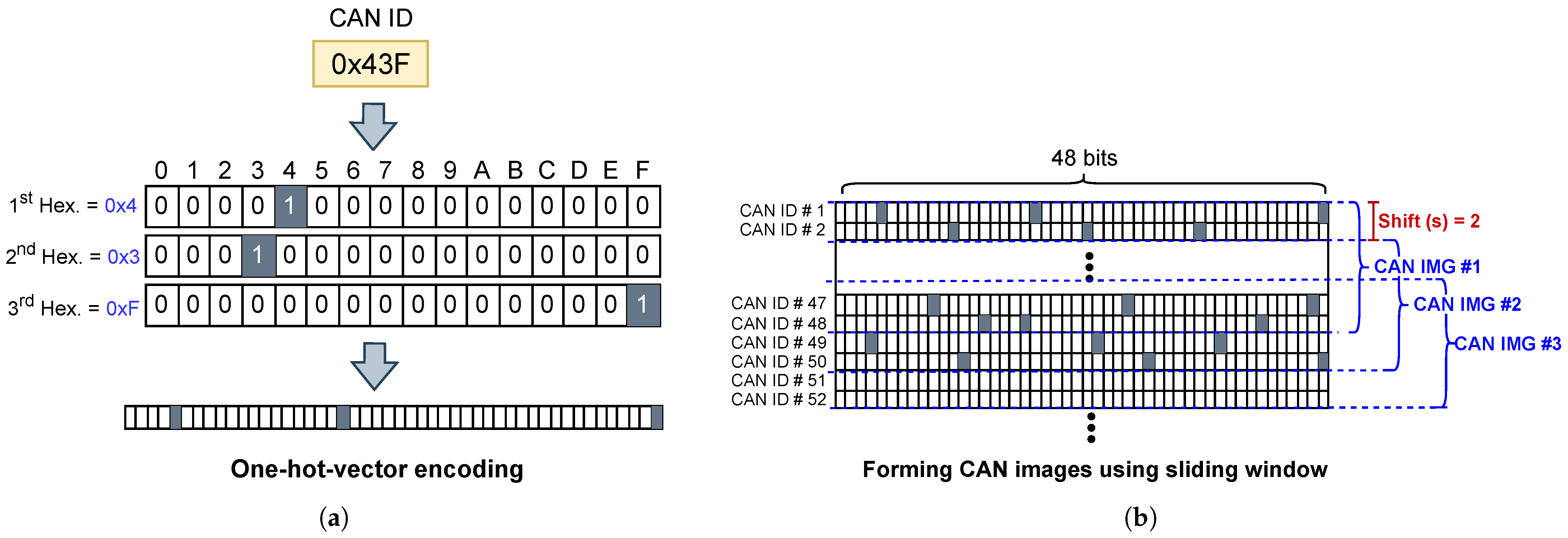
• A sliding-window technique is implemented during CAN message encoding to increase the amount of data. This technique improves detection accuracy by up to 0.66%, as demonstrated through experiments on three datasets extracted from different vehicles.
• A proposed network pruning process is applied to BNN-based IDS models trained on these three datasets. The pruned models achieve up to 91.07% parameter reduction while maintaining near-identical accuracy, with only a 0.01% drop.
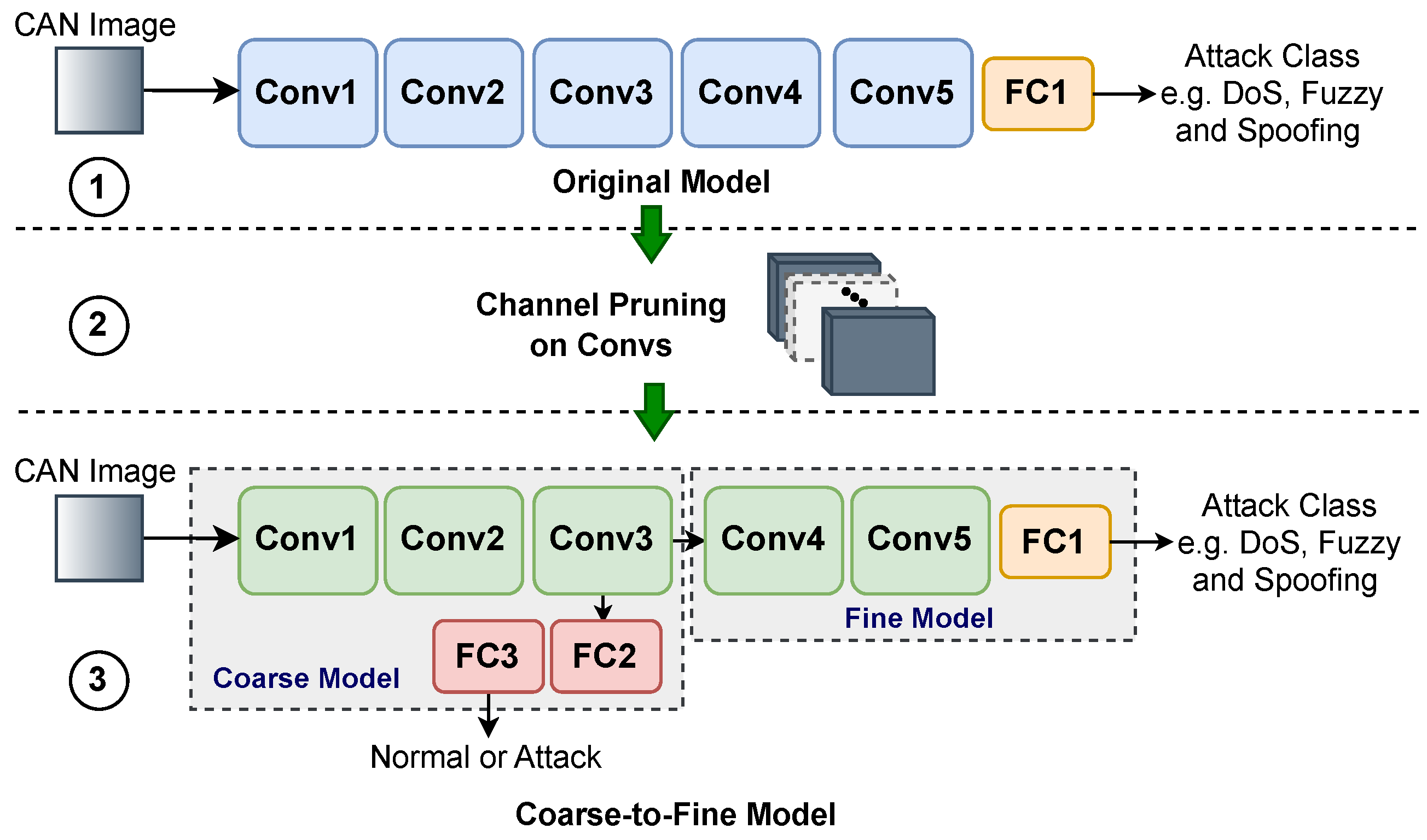
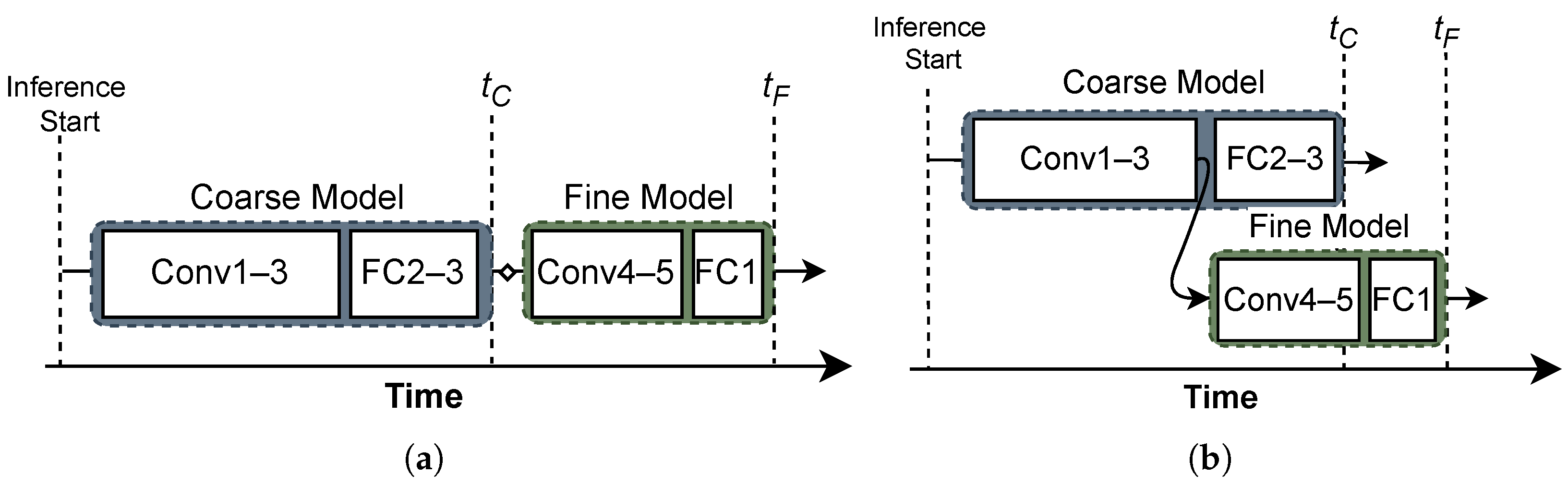
• The developed models are then structured using the Coarse-to-Fine (C2F) approach, which further reduces inference time by allowing the Coarse model to perform initial attack detection, while the Fine model is executed only when an attack is detected for classification. This approach saves inference time by up to 19.3% on GPU and 33% on FPGA when no attack is detected.
• The developed BNN-based IDSs are implemented on CPU, GPU, and FPGA platforms using state-of-the-art frameworks to fully exploit their computational efficiencies. The FPGA implementation demonstrates superior performance, outperforming GPU and CPU implementations by up to 3.7× and 2.4× in speed, while achieving up to 7.4× and 3.8× greater energy efficiency, respectively.

The rest of this paper is organised as follows: Section 2 provides background knowledge on the structure of CAN messages, CAN bus vulnerabilities, and the public datasets used in this study. BNN-based IDSs are also explored in this section. Section 3 discusses how network pruning can be applied to BNNs, the proposed pruned BNN-based IDSs, and their deployment across different platforms using the state-of-the-art frameworks. Then, Section 4 presents the experimental results. Finally, Section 5 concludes the paper.

2. Background and Related Work

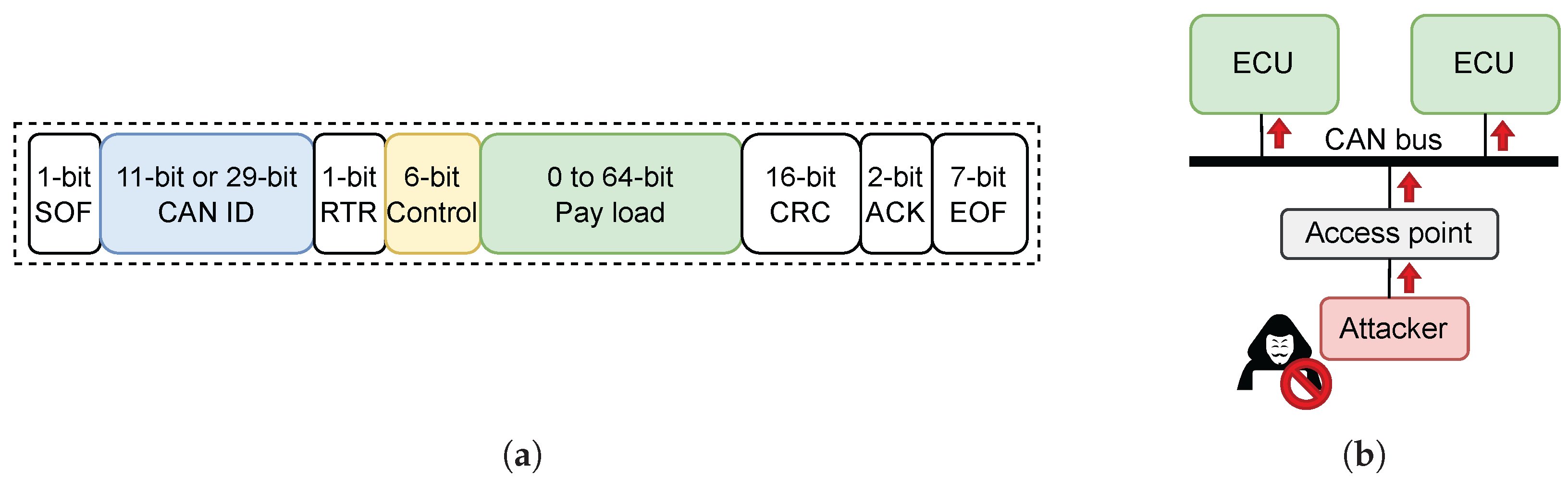
2.1. CAN Message and Injection Attack Datasets

CAN is a message-based broadcast protocol widely used in vehicles. It utilises twisted-pair cables, known as CAN-high and CAN-low, which enhance noise resistance while keeping costs low. Since CAN operates as a broadcast communication bus, when an ECU or a node transmits a message on the CAN bus, all other ECUs within the network receive the transmitted message simultaneously.

Figure 1a presents the bit-wise structure of a CAN message. A CAN message consists of the following components: 1-bit Start of Frame (SOF), CAN Identifier (CAN ID), 1-bit Remote Transmission Request (RTR), 6-bit control field, Payload, 16-bit Cyclic Redundancy Check (CRC), 2-bit Acknowledge (ACK), and 7-bit End of Frame (EOF). The CAN ID field can be either 11 bits (standard format) or 29 bits (extended format). The control field includes the Data Length Code (DLC), which specifies the size of payload in bytes. The payload (data field) can be up to 8 bytes (64 bits). On a CAN bus, each bit is either dominant (0) or recessive (1), with dominant bits taking priority over recessive bits in the event of a collision.

As shown in Figure 1b, an attacker can gain access to a vehicle’s CAN bus through various entry points, such as the OBD-II port, infotainment system, wireless telematics unit, or by directly tapping into the CAN bus wires. Once connected, attackers can exploit the broadcast nature of the CAN bus by simply injecting fabricated messages, potentially manipulating critical vehicle functions. In this work, message-injection attacks are categorised into four types: Denial of Attack (DoS), Fuzzy, Spoofing, and Replay attacks. When a CAN bus is under DoS attack, attackers flood the CAN bus with highest-priority messages (e.g., CAN ID: 0x000), preventing valid messages from reaching their destination nodes. In Fuzzy attack, intruders inject CAN messages with random CAN IDs, often as part of reverse-engineering attempts. In Spoofing, the attackers, having identified specific CAN IDs, inject fraudulent messages to control vehicle functions. Lastly, Replay attack involves capturing valid CAN messages and reinjecting them with the same CAN IDs to deceive the vehicle.

To comprehensively evaluate the effectiveness and efficiency of our optimised IDSs, we utilised three datasets captured from different vehicles, as summarised in

Table 1. Summary of injection-attack datasets used in this study.

Dataset	Year	Vehicle	# Messages	# Attacks
Car Hacking (CH) [18]	2018	Hyundai YF Sonata	17,558,462	4
Survial Analysis (SA) [19]	2018	Chevrolet Spark	402,956	3
Attack & Defense Challenge (ATK&DEF) [20]	2021	Hyundai Avante CN7	7,424,197	4

. The details of each dataset and its attack types are as follows:

• The first dataset, known as the Car-Hacking dataset (CH) [18], collected from a Hyundai FY Sonata, includes four attack types: DoS, Fuzzy, Gear Spoofing, and RPM Spoofing. During a DoS attack, messages with CAN ID 0x000 were injected every 0.3 ms to flood the network. For the Fuzzy attack, both CAN IDs and payloads were randomly generated, with messages injected at an interval of 0.5 ms. As the names of attacks imply, for Gear Spoofing and RPM Spoofing, messages with CAN IDs responsible for displaying gear position and speed gauge in RPM (revolutions per minute) were injected every 1 ms to manipulate these vehicle functions.
• The second dataset, part of the Survival Analysis Dataset (SA) [19], was extracted from a Chevrolet Spark, and comprises three attack types: DoS, Fuzzy, and Spoofing. Again, during DoS attack, messages with CAN ID 0x000 were injected to overload the network. During Fuzzy attack, messages with random CAN IDs ranging from 0x000 to 0x7FF were injected every 0.3 ms. Messages with a specific CAN ID (0x18E) were injected to deceive the vehicle’s systems during the Spoofing attack.
• The third dataset, collected from a Hyundai Avante CN7 in the Attack & Defense Challenge (ATK&DEF) [20], contains four attack types: DoS, Fuzzy, Spoofing, and Replay. The CAN messages were captured in both driving and stationary states, with preliminary round data used in this study. The DoS and Fuzzy attacks involve sending messages with the highest priority CAN ID (0x000) and random CAN IDs, respectively. Various Spoofing attacks were performed, including factory-mode warning, RPM gauge manipulation, engine-off warning, blind-spot collision warning, and rear-camera activation. During the Replay attack, previously captured CAN messages were re-injected into the network at a later time to mimic legitimate activity.

2.2. Related Work on BNN-Based IDSs

BNNs use −1 and 1 as parameters [12], which can be represented using a single bit, where 0 represents −1 and 1 represents 1. Compared to conventional 32-bit floating-point neural networks, this reduces the memory required for storing parameters by 32×, making BNNs highly lightweight. Additionally, since BNN execution involves simple XNOR operations followed by popcount, the inference process is both fast and computationally inexpensive.

Given these advantages, BNNs have been explored for efficient CAN IDS development. In [13], a BNN-based IDS was proposed using a three-layer fully connected (FC) architecture, where each FC contained 1024 nodes and was connected to batch normalisation [21] and dropout layers [22] to mitigate overfitting. The model’s input was generated by concatenating the 11-bit CAN IDs and 64-bit payloads from 10 consecutive messages, along with 34 zero-padding values, forming a 28 × 28 grid frame. The developed model was evaluated across CPU, GPU, and FPGA platforms to determine the most efficient deployment.

To enhance accuracy, Binarised Convolutional Neural Network (BCNN) were introduced in [14], incorporating convolutional layers (Convs), with evaluation conducted on a GPU. To generate an input, the DeepInsight framework [23] was utilised to construct images. These generated images were built based on both CAN IDs and payloads from 128 consecutive CAN messages.

In [15], a two-stage BNN-based IDS, called Coarse-to-Fine (C2F), was proposed and implemented on an FPGA. This method takes a 30 × 30 CAN image as input, generated by binary encoding 30 CAN IDs. The first stage, the Coarse model, detects attacks, while the second stage, the Fine model, classifies the detected attacks. The C2F-based IDS enhances inference efficiency, as most CAN messages are normal and do not require the unnecessary processing in the second stage. The C2F concept was further extended in [16], named BNN-based IDS (BIDS), which enables unknown attack detection by incorporating a Generative Adversarial Network (GAN) discriminator head. To maximise inference efficiency, the Coarse and Fine models are executed in parallel. The input consists of a stack of 48 one-hot encoded CAN IDs from consecutive messages, forming an optimised CAN image. Implemented on an FPGA, BIDS achieves real-time operation, offering the fastest inference speed among IDS solutions capable of detecting both known and unknown attacks while maintaining comparable accuracy.

In this work, we adopt the C2F-based IDS, further optimise it, and conduct a comprehensive evaluation. One-hot vector encoding is chosen to convert CAN IDs into CAN images due to its simplicity and effectiveness, as demonstrated in [16,18,24]. This encoding is particularly suitable for BNNs, as it produces only 0 s and 1 s, ensuring no information loss during input quantisation. While various platforms for BNN-based IDS implementation were compared in [13], only the FPGA implementation fully utilised the simplified operations of the BNN. To provide a fair and comprehensive comparison in this work, we evaluate the developed BNN-based IDSs across CPU, GPU, and FPGA, applying BNN execution optimisations specific to each platform using state-of-the-art frameworks, which will be discussed in Section 3.4. Moreover, network pruning was implemented and assessed on three BNN models using three different datasets, to ensure that the proposed models are effective and fully optimised.

Table 2. Comparison of BNN-based IDS approaches in related work.

Model	Input	Classifier	Key Techniques
BNN-FCs, 2022  [13]	ID, Payload	Binary	Evaluation on CPU, GPU, and FPGA
BCNN, 2024 [14]	ID, Payload	Binary	DeepInsight [23] for image formation
BNN-C2F, 2024 [15]	ID	Multiclass	Coarse-to-Fine (C2F) model
BIDS, 2024 [16]	ID	Multiclass	GAN for unknown attack detection
This work	ID	Multiclass	Pruning with CPU, GPU, and FPGA evaluation

summarises the key distinctions between our work and previous studies.

3. Proposed Pruned BNN-Based IDSs

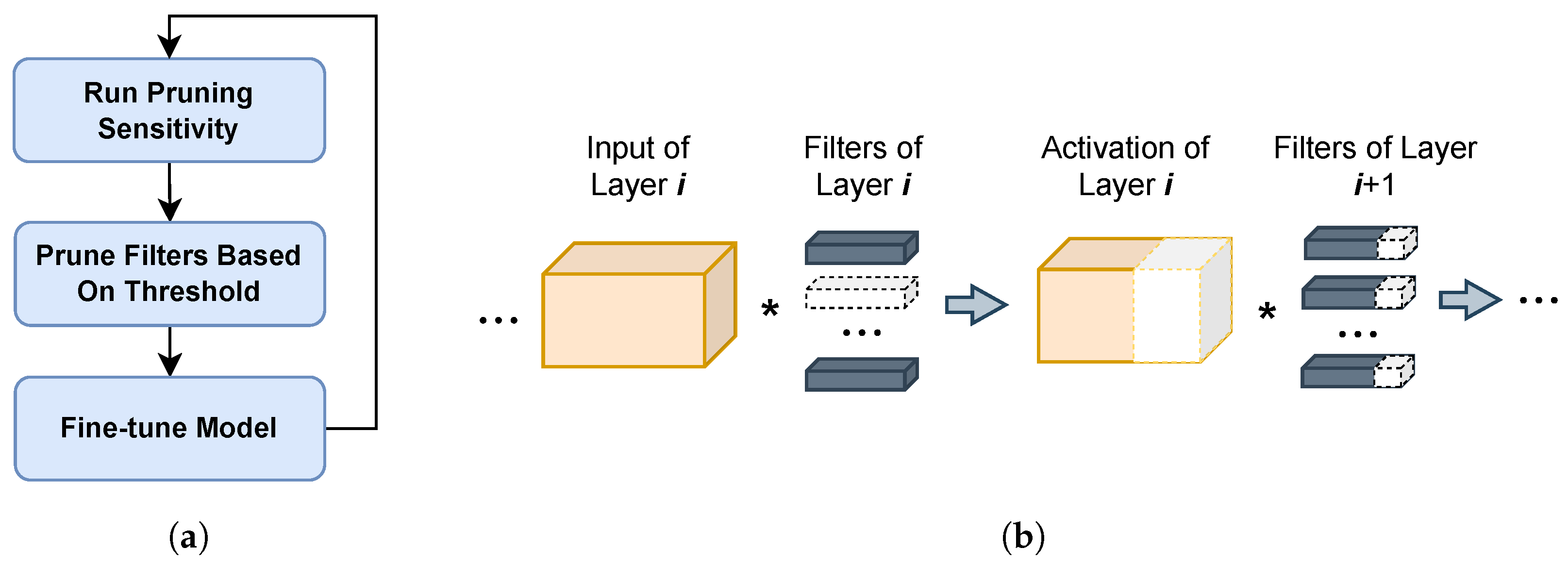
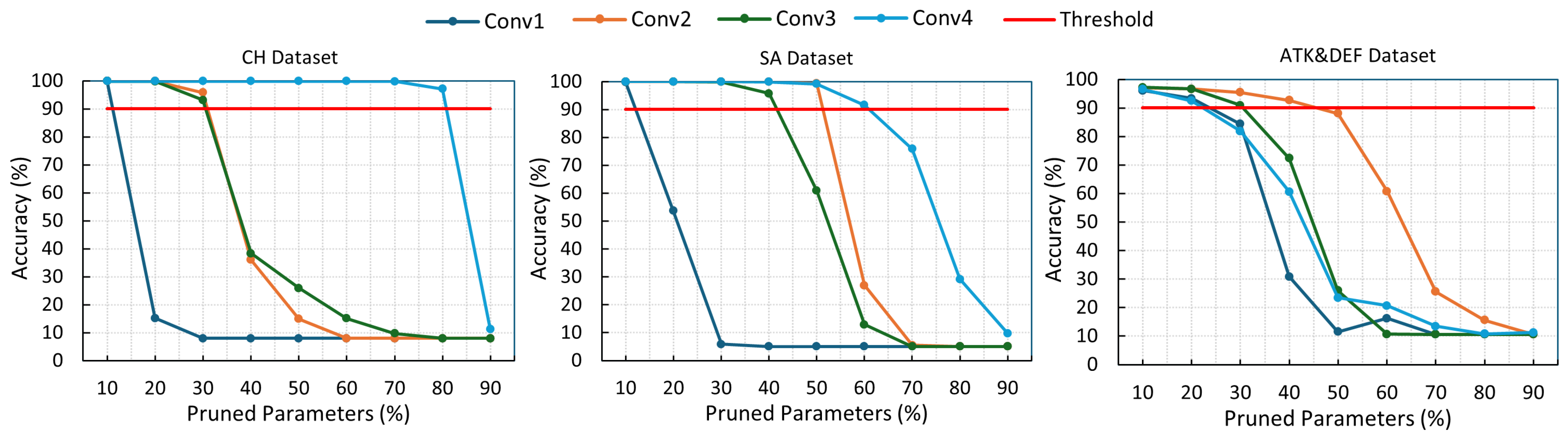
3.1. Network Pruning for BNNs

Network pruning is a model compression technique that eliminates redundant or unnecessary structures based on specific evaluation criteria. Various levels of pruning granularity exist [25], ranging from fine-grained pruning [26,27,28] to channel-level pruning [29,30]. Generally, coarse-grained pruning, such as channel-level pruning, results in more hardware-efficient models by enabling structured and regular computations, leading to faster inference.

Selecting an appropriate pruning metric is crucial for assessing the importance of parameters. In BNNs, pruning based on the direct value of weights is ineffective since BNN weights are restricted to −1 and 1, making all weights appear equally significant. To address this, in [31], rather than relying on the actual weight values, the frequency of weight flipping is observed during the final stage of training. Parameters with the highest flipping frequency are pruned away, as they are assumed to have a minimal contribution to the model’s overall accuracy.

During BNN training, 32-bit floating point (real-valued) weights are maintained alongside their binarised counterparts to improve learning effectiveness. During forward propagation, the binarised weights are used for loss calculation and inferences. In the backward pass, the real-valued weights are updated based on the calculated gradients, after which the binarised weights are adjusted accordingly. In [32], the importance of filters is assessed by measuring the distance between real-valued weights and their quantised counterparts. To measure this distance, cosine similarity is employed and the results have been shown to be effective for pruning less important weights of BNNs. This metric helps identify filters that are less affected by quantisation, as those with smaller distances between their real and quantised versions are likely to retain their representational power post quantisation. Conversely, weights with larger distances are more prone to flipping between quantised values during training, indicating that they contribute less to the model’s overall performance.

In this paper, we adopt a pruning approach similar to [32], using cosine similarity as the pruning metric to measure the distance between real-valued and quantised filters weights. Pruning is performed at the channel or filter level to maximise inference speed improvements on hardware implementations without requiring additional specialised operations. To assess filter importance at the channel level, each filter is vectorised and evaluated using the cosine similarity function, defined as:

$$S_C(r,q)={\displaystyle \frac{r·q}{\parallel r\parallel \parallel q\parallel }}$$

(1)

where r and q are 1 − D vectors representing the real-valued and quantised filter weights, respectively. A lower cosine similarity indicates a greater distance between the two representations, suggesting that the filter contributes less to the model’s performance and can be pruned.

3.2. Developing BNN-Based IDSs

The proposed BNN-based IDS is built upon the model from [16], which originally consists of five convolutional layers (Convs) and one fully connected layer (FC), as illustrated in step 1 of Figure 2. Each Conv and FC layer is followed by a batch normalisation layer [21] to improve model stability and accuracy. Conv1 outputs 48 channels with a kernel size of 3, stride of 2, and padding of 1. Conv2, Conv3, and Conv4 produce 96, 96, and 192 output channels, respectively, using the same kernel, stride, and padding parameters as Conv1. Conv5, the final convolutional layer, maintains an output of 192 channels, with a stride adjusted to 1 and no padding applied. Batch normalisation is applied after each convolution, followed by a sign activation (binarisation) function. The output of the final convolutional layer is then flattened and passed to FC1, which produces an output corresponding to the number of attack classes. Therefore, for the CH dataset, FC1 outputs five classes: Normal, DoS, Fuzzy, Gear Spoofing, and RPM Spoofing. Similarly, the outputs of FC1 for the ATK&DEF dataset consist of five classes: Normal, DoS, Fuzzy, Spoofing, and Replay. For the SA datatset, the outputs correspond to four classes: Normal, DoS, Fuzzy and Spoofing. The original model was trained for 50 epochs, starting with a learning rate of 0.01, which was halved every five epochs. The model achieving the highest accuracy was selected for evaluation.

As shown in step 2 of Figure 2, channel pruning (described in the next subsection) is applied to the original model to remove unnecessary parameters. In Step 3, the pruned model is then restructured into a two-stage Coarse-to-Fine (C2F) model to enhance inference efficiency. The key idea behind C2F is to execute the second stage only when necessary, thereby reducing computational overhead. Specifically, the second stage is activated only when an attack is detected, allowing it to classify the attack type. In the first stage, two additional fully connected layers (FC2 and FC3) are introduced and connected to Conv3, forming the Coarse model. Since the stage is responsible for attack detection, it is fine-tuned using a dataset labelled with only two classes: Normal and Attack. During this process, the parameters of Conv1, Conv2, and Conv3 are frozen, allowing only the parameters of FC2 and FC3 to be updated. The training parameters for fine-tuning, including the learning rate and number of epochs, remain identical to those used for the original model. The second stage, comprising Conv4, Conv5, and FC1, is referred to as the Fine model. It retains the exact parameters of the original model and processes the output of Conv3 to classify the detected attack type.

To build an input that captures the sequential patterns of CAN IDs, 48 consecutive CAN IDs are encoded using a one-hot vector method, similar to [18,24], forming a 48 × 48 CAN image. Figure 3a illustrates encoding process for the CAN ID 0x43F using this method. Each hexadecimal digit of the CAN ID is independently converted into a 16-bit one-hot vector. In this example, the hexadecimal digits 4, 3, and F are encoded by setting the fourth, third, and sixteenth bits to 1, while all other bits remain 0.

These three one-hot vectors are then concatenated to create a 48-bit sequence. To generate a 48 × 48 CAN image, this 48-bit sequence is stacked with 47 additional encoded CAN IDs, as shown in Figure 3b. A CAN image containing at least one attack message is labelled with its corresponding attack type. Building on the work of [18,24], this study also implements a sliding window (SW) method to overlap CAN IDs during the formation of encoded CAN images. This approach extends the size of encoded data, providing more training samples for the IDS and improving model accuracy. The shifting value (s) determines the extent of overlap between successive CAN images. For example, the SW implementation with the s value of 2, as shown in Figure 3b, uses 46 overlapping CAN IDs to create the first CAN image, and the window then shifts by two CAN IDs to generate the next image.

Ideally, to generate the maximum number of images, the sliding-window shift value (s) should be set to 1, producing CAN images nearly equal in number to the available CAN messages. However, for datasets with a large number of CAN messages (e.g., 17 million messages), creating images at this scale can lead to excessive memory usage and significantly increased training time. To balance efficiency and dataset size, different s values were chosen. For the CH dataset (the largest dataset), we selected s = 24 to approximately double the number of CAN images compared when no SW method was applied. For the ATK&DEF dataset, s = 12 was chosen to increase the number of images by approximately four times, and for the SA dataset (smallest dataset), s = 1 was used to maximise the number of generated images. To prevent duplicate CAN images, the uniqueness of each image was checked during encoding.

3.3. Pruning Models

The proposed pruning process consists of three steps, as illustrated in Figure 4a. The first step is to run pruning sensitivity by pruning each convolutional layer individually, and measuring the corresponding drop in model accuracy. Layers that cause significant accuracy degradation when pruned are considered sensitive and are assigned lower pruning ratios to maintain overall accuracy of the model. The second step involves pruning the model with the ratios that preserve the accuracy above a certain threshold, which is set to 90% in this work. The final step is to fine-tune the pruned network to recover the model accuracy. To ensure accurate attack detection, these steps are repeated iteratively until the accuracy of the model after fine-tuning drops by more than 0.01%.

Figure 4b illustrates the filter pruning approach used to reduce the number of activation channels in layer i. Similar to [32], the pruning metric in Equation (1) is applied to the input channels of filters in layer i + 1. Filters corresponding to less important channels are pruned first, based on a specified pruning ratio. For example, if the target pruning ratio is 30%, channels are ranked from least to most important, and the bottom 30% are eliminated. Furthermore, since input channels in layer i + 1 are removed, the corresponding filters in the previous layer (the output channels of layer i) are also eliminated.

The results of the first iteration of pruning sensitivity for each dataset are shown in Figure 5, illustrating how accuracy drops as parameters are pruned from each layer individually. For the CH and SA datasets, the first layer (Conv1) is the most sensitive to pruning, while the deepest layer (Conv4) is relatively insensitive and can be pruned at a higher ratio without significantly affecting model performance. In contrast, for the ATK&DEF dataset, the model tends to be equally sensitive to pruning across all layers. The pruning ratios are determined based on the highest values that still maintain accuracy above the 90% threshold, as indicated by the red line. Therefore, in this first iteration, the selected pruning ratios for the CH dataset model are 10%, 30%, 30% and 90% for Conv1, Conv2, Conv3 and Conv4, respectively. For the SA dataset, the chosen ratios are 10%, 50%, 40% and 60%, while for the ATK&DEF dataset, they are 20%, 40%, 30% and 20%. After pruning, the model is fine-tuned for 20 epochs, and then the next iteration begins by running pruning sensitivity on the retrained pruned model.

The decision to select a 90% accuracy threshold for pruning is based on the pruning sensitivity observed during the first iteration for the CH and SA datasets. In the CH dataset, reducing the threshold from 90% to 40% results in no change in pruning ratios across layers. Further lowering it to 30% affects only Conv2 and Conv3, requiring an additional 10% pruning each, but this leads to a steep drop in overall accuracy, from above 90% to below 40%. A similar trend is observed in the SA dataset, where even a 10% increase in pruning beyond the 90% accuracy threshold causes a significant decline in model performance. For instance, increasing the pruning ratio of Conv3 from 40% (at the 90% accuracy threshold) to 50% results in a drop in model accuracy from above 90% to approximately 60%. These findings indicate that lowering the threshold below 90% offers negligible gains in pruning efficiency while considerably compromising model accuracy.

3.4. Hardware Implementation Frameworks

To identify the most efficient deployment solution for BNN-based IDS, various platforms, including CPU, GPU and FPGA, are targeted and compared in terms of power consumption and inference time. Given that BNN involves specialised operations like XNORs and popcounts, it is crucial to select an appropriate framework that efficiently utilises these operations. Therefore, state-of-the-art frameworks for implementing BNN across different hardware platforms and their utilisation in executing C2F-based models are explored in this subsection.

3.4.1. CPU-Based BNN with Larq Compute Engine

Larq Compute Engine (LCE) [33] is selected for deploying our BNN-based IDS due to its superior inference speed compared to other existing frameworks, such as TVM [34] and DaBNN [35]. LCE is an open-source framework built as an extension of Tensorflow Lite (now LiteRT) [36], allowing users to utilise its existing features for high performance deployment. Larq [37], which is also based on Tensorflow [38], facilitates BNN training and seamless conversion of trained models to LCE for inferences. LCE optimises instruction sets for executing Binary General Matrix Multiplication (BGEMM), enabling 1024 binary MAC operations with just 24 instructions in BNN convolutional layers. For inference, LCE stores each binary weight using only a single bit, fully exploiting the compact nature of BNNs. LCE supports 64-bit ARM-based platforms, such as the Pixel 1 phone and Raspberry Pi.

For deploying the C2F-based IDS, the Coarse and Fine models are exported separately using the LCE converter. The models are modified according to the guidelines in the LCE optimisation guide [39], where fully connected layers are excluded for binary operation optimisation and replaced with 1 × 1 convolutional layers. The models are then integrated into a single C++ file, where the Coarse model runs first. If an attack is detected, the Fine model is executed sequentially to determine the attack type, as shown in Figure 6a. In contrast, if no attack is detected by the Coarse model, the execution of the Fine model is skipped, allowing the IDS to immediately process the next CAN image after the Coarse model produces its result.

3.4.2. GPU-Based BNN with Bit-Tensor Cores

Bit-Tensor Core (BTC) [40] utilises Tensor Cores technology [41] in NVIDIA GPUs to accelerate BNN executions. It optimises BNN operations by replacing traditional MAC computations with XNOR followed by popcount and by combining batch normalisation and sign activation into a simple threshold. Moreover, the fixed stride of memory access is carefully determined to optimise memory access performance. BTC is implemented on GPUs with Turing architecture across six different BNN models. It compares the results with state-of-the-art BNN designs and demonstrates its superior performance. The implementations are developed in CUDA and published online for further research.

For the BNN-based IDS evaluation, models are built using available functions and existing code. Similar to the CPU-based implementation, as shown in Figure 6a, the C2F-based IDS on the GPU first executes the Coarse model, followed by the Fine model if an attack is detected.

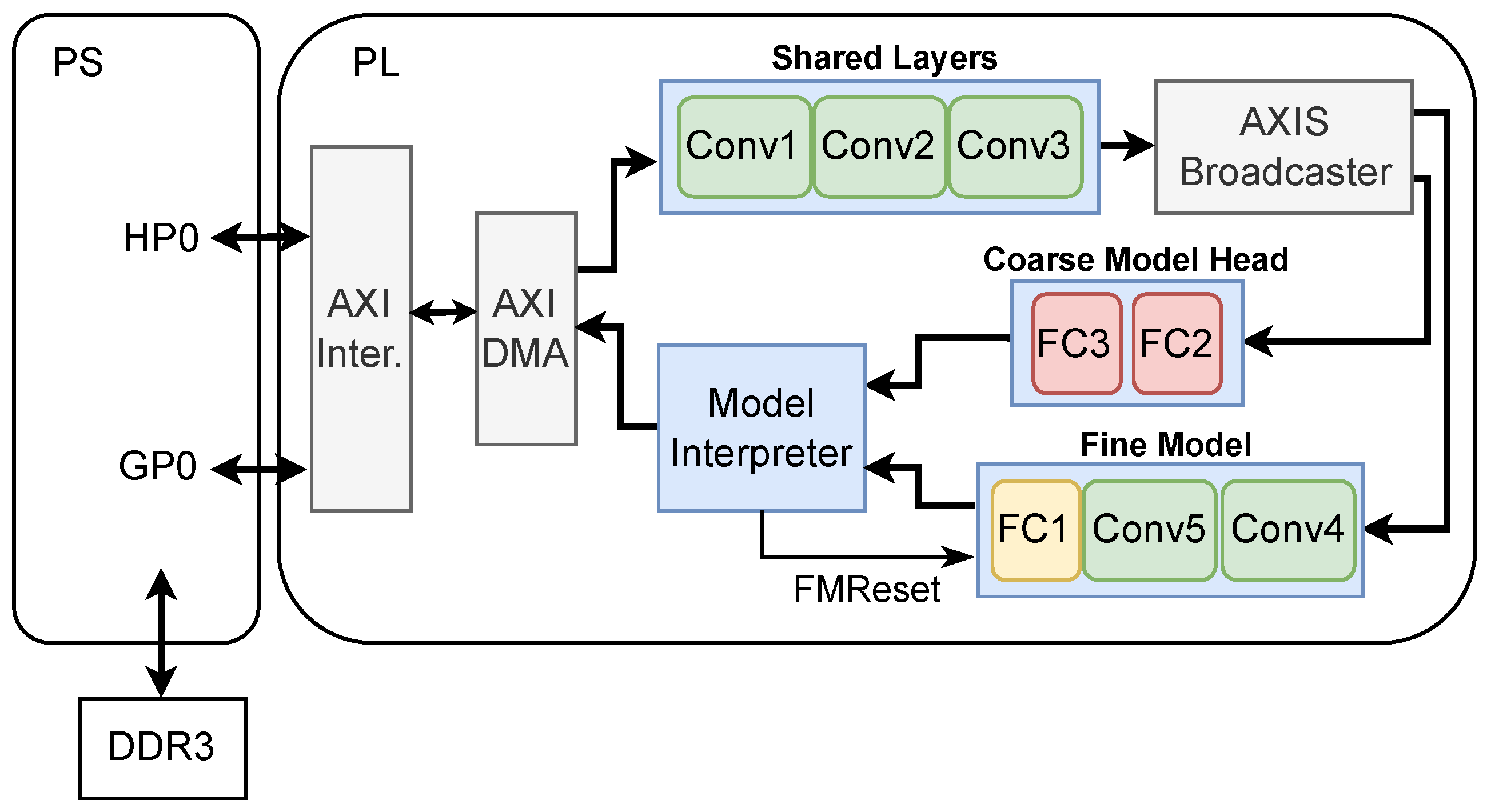
3.4.3. FPGA-Based BNN with FINN

The FINN automation framework [42,43] enables efficient deployment of a developed BNN onto an FPGA using Python 3, a widely-used high-level ML programming language. Since BNN parameters are small, they fit within on-chip memory, eliminating bottlenecks associated with external memory access and enabling high-performance inference. FINN builds compute arrays for each layer based on user requirements, incorporating simplified XNOR, popcount operations, and thresholding. This approach avoids a one-size-fits-all model and fully exploits the reconfigurable nature of FPGAs.

Brevitas [44], a Pytorch library developed by Xilinx, facilitates BNN development and evaluation while ensuring seamless model export in a format compatible with the FINN compiler. FINN allows users to estimate resource utilisation and inference speed layer by layer, eliminating the need to implement the actual model on an FPGA for preliminary evaluation. This enables quick experimentation with various configurations. The generated compute blocks follow a dataflow architecture and use AXI-Stream [45] for inter-block communication.

To implement the C2F-based IDS, the approach in [16] is adopted. The Coarse and Fine model are converted into FPGA IP blocks through the FINN automation process for bare-metal execution. The IDS architecture is designed so that the Coarse and Fine models can run in parallel, as illustrated in Figure 6b. In addition, when the Coarse model detects no attacks, the Fine model can be reset on the fly, allowing the next CAN image to be immediately fed into the models for inference.

4. Validation and Experimental Results

4.1. Experimental Setup

BNN-based IDSs were trained, evaluated, and pruned using Brevitas [44] and PyTorch [46]. As described in Section 3, the BNNs were initially trained using the original model structure across three different datasets. The pruning process was then applied, followed by training the Coarse model to establish the C2F structure. Finally, the models were deployed on three platforms, CPU, GPU, and FPGA, to evaluate and compare power consumption and inference time.

To ensure efficient execution of BNNs’ simplified operations, the most suitable framework was selected for each platform, as previously described. The hardware platforms and their corresponding frameworks are as follows:

• CPU—Raspberry Pi 5 [47]: A 64-bit quad-core Arm Cortex-A76 processor, using Larq Compute Engine (LCE) version 0.13.0.
• GPU—Jetson Orin Nano [48]: 1024-core NVIDIA Ampere architecture GPU with 32 Tensor Cores, using Bit-Tensor Core (BTC).
• FPGA—Zedboard [49]: Xilinx Zynq 7000 System-On-Chip (SoC), using FINN version 0.10 and Xilinx Vivado 2022.2.

4.2. Pruned Model Accuracy

The encoded dataset was split into training and testing sets with an 80:20 ratio.

Table 3. Comparison of model accuracy with and without the sliding-window approach across different datasets.

Dataset	Shift (s)	# CAN Images w/o SW		# CAN Images with SW		Acc. (%) w/o SW	Acc. (%) with SW
		Normal	Attack	Normal	Attack
CH—Hyundai YF Sonata	24	232,838	132,539	450,914	265,026	99.91	99.94
ATK&DEF— Hyundai Avante CN7	12	47,693	28,807	189,083	115,114	96.98	97.64
SA—Chevrolet Spark	1	6181	2212	257,648	104,346	99.76	99.99

presents a comparison of the model accuracy after training with and without the sliding window (SW) implementation. Incorporating the SW method leads to improved accuracy across all datasets due to the increased number of training samples. Specifically, the model accuracy of the CH dataset improves slightly by 0.03% with the SW method, while the improvements of the SA dataset and ATK&DEF dataset are 0.23% and 0.66%, respectively. These results highlight that expanding the dataset using the SW technique enhances the model’s ability to generalise, particularly for smaller datasets where limited samples can negatively impact performance.

Table 4. Pruning results for each dataset.

Dataset	# Iterations	Acc. (%)	ΔAcc. (%)	Reduced Params (%)
CH	3	99.93	−0.01	91.07
SA	3	99.98	−0.01	87.51
ATK&DEF	1	96.51	−1.13	33.39

presents the accuracy of each dataset using the original model structure after applying the pruning process discussed in Section 3.3. For the CH and SA datasets, 91.07% and 87.51% of the model parameters can be pruned after three iterations, with only a 0.01% drop in accuracy. In contrast, for the ATK&DEF dataset, pruning after just the first iteration results in a 1.13% drop in accuracy, with 33.39% of the parameters pruned. Consequently, the model trained on the ATK&DEF dataset is considered unsuitable for pruning, so we decided to use the original model for further experiments. The decline in accuracy for the ATK&DEF dataset may be due to the nature of Replay and Spoofing attacks, both of which involve injecting functional CAN IDs and disturbing the normal flow of CAN IDs in similar ways. The BNN may lack the capacity to effectively distinguish these subtle differences.

Table 5. Details of pruned parameters and activations in CH and SA datasets.

Layer	# Original Params	Params Pruned		# Original Activations	Acts Pruned
		CH	SA		CH	SA
Conv1	0.4 k	18.8%	27.1%	27.6 k	18.8%	27.1%
Conv2	41.5 k	54.3%	81.8%	13.8 k	43.8%	75.0%
Conv3	82.9 k	80.7%	92.5%	3.4 k	65.6%	69.8%
Conv4	165.9 k	98.2%	94.9%	1.7 k	94.8%	83.3%
Conv5	331.8 k	94.8%	83.2%	0.2 k	0%	0%
Total	622.5 k	91.1%	87.5%	46.8 k	32.3%	46.3%

presents the number of parameters and activations in each convolutional layer for CH and SA datasets. The total number of parameters in the convolutional layers is reduced from 622.5 k to 55.6 k for the CH dataset and to 77.8 k for the SA dataset, corresponding to reductions of 91.1% and 87.5%, respectively. Notably, the deeper layers of the CH model are pruned at slightly higher percentages than those of the SA model. Since most parameters reside in the deeper layers, the pruned CH model has fewer total parameters. In contrast, the shallower layers of the SA model, particularly Conv2, undergo more pruning. Although these shallow layers contain fewer parameters, they generate a larger number of activations compared to the deeper layers. Since activations serve as inputs for subsequent layers, reducing their number helps lower both computational cost and memory usage for intermediate results during inference.

The pruned models for the CH and SA datasets, along with the original model for the ATK&DEF dataset, are then reconstructed into the C2F structure, as discussed in Section 3. To effectively assess an IDS, especially when dealing with imbalanced datasets, evaluation metrics such as precision, recall, and F1 score are measured in addition to accuracy. These metrics are computed using true positives (TP), true negatives (TN), false positives (FP), and false negatives (FN). In this context, TP and TN represent correctly identified attack (positive class) and normal (negative class) instances, respectively. FP and FN refer to a normal instance incorrectly classified as an attack (positive class), and attack as a normal (negative class) instance, respectively.

The One-vs-Rest approach is used to calculate these metrics for multiclass classification. In a multiclass classification setting with k-class outputs, the precision ($P_i$), recall ($R_i$) and F1 score ($F1effiscor{e}_i$) for class i, where each class 1 ≤ i ≤ k is treated as the positive class, are defined as follows:

$$Precision\left(P_i\right)={\displaystyle \frac{T{P}_i}{T{P}_i+F{P}_i}}$$

(2)

$$Recall\left(R_i\right)={\displaystyle \frac{T{P}_i}{T{P}_i+F{N}_i}}$$

(3)

$$F1scor{e}_i={\displaystyle \frac{2\times (P_i\times R_i)}{P_i+R_i}}$$

(4)

The negative class is defined as the sum of all other classes. Therefore, when evaluating attack class i (the positive class), the normal class and all other attack classes are treated as the negative class. It is important to note that the F1 score is widely used to evaluate the effectiveness of imbalanced classification systems, as it incorporates both precision and recall, providing a balanced measure of model performance.

Table 6. Effectiveness of C2F-based IDSs across three datasets.

Dataset	Attack	Accuracy (%)	Precision (%)	Recall (%)	F1 (%)
CH (Pruned)	DoS	99.92	99.98	99.88	99.93
	Fuzzy		99.99	99.65	99.82
	Spoofing RPM		99.97	99.81	99.89
	Spoofing Gear		99.98	100	99.99
SA (Pruned)	DoS	99.96	100	99.95	99.98
	Fuzzy		99.97	99.70	99.84
	Spoofing		100	99.80	99.90
ATK&DEF (Original)	DoS	96.96	100	99.66	99.83
	Fuzzy		97.94	95.18	96.54
	Spoofing		92.26	85.71	88.86
	Replay		97.46	86.40	91.60

and

Table 7. Confusion matrices of C2F-based IDSs across three datasets.

Dataset	Attack	TP	TN	FP	FN
CH (Pruned)	DoS	9165	125,827	2	11
	Fuzzy	10,732	124,235	1	37
	Spoof RPM	15,944	119,026	5	30
	Spoof Gear	17,252	117,731	3	19
SA (Pruned)	DoS	11,064	61,330	0	5
	Fuzzy	3633	68,754	1	11
	Spoofing	6080	66,307	0	12
ATK&DEF (Original)	DoS	7337	53,478	0	25
	Fuzzy	6125	54,276	129	310
	Spoofing	3208	56,828	269	535
	Replay	4760	55,207	124	749

present the effectiveness and confusion matrices of the C2F-based IDSs for each dataset, respectively. It is important to note that the models for the CH and SA datasets are pruned, whereas the original model structure is used for the ATK&DEF dataset, as pruning significantly impacts its accuracy. The C2F model enhances efficiency by introducing the Coarse model, which has fewer parameters and can be executed quickly, while the Fine model is used only when necessary. However, after implementing the C2F structure, the accuracy of the C2F-based IDS slightly decreases for both the SA and CH datasets. This drop occurs because the overall performance depends on the Coarse model’s accuracy, which contains fewer parameters. The negative impact is even worsened for the ATK&DEF dataset. Thus, this trade-off between efficiency and accuracy should be carefully taken into account when implementing this approach.

Overall, the models for the CH and SA datasets demonstrate high effectiveness, achieving F1 scores exceeding 99% for all attack classes. In contrast, the F1 score for the ATK&DEF dataset reaches only 88.86% for the Spoofing class. As previously discussed, this low performance is likely due to the similarity between Spoofing and Replay attacks, as both involve injecting valid CAN IDs into the vehicle network, making them more difficult to distinguish. If distinguishing between these two attacks is required, increasing the model’s bit precision is recommended, as it enhances the model’s capacity to capture subtle differences.

For clarity and simplicity in discussing inference time and power consumption, the original model without pruning is referred to as “Original”. “Original-C” denotes executing only the Coarse model with the original structure, while “Original-C&F” represents running the Coarse and Fine models sequentially on the CPU and GPU, and in parallel on the FPGA. Similarly, “CH-Pruned” and “SA-Pruned” refer to the pruned models for the CH and SA datasets, respectively. Their C2F execution counterparts are denoted as: “CH-C-Pruned” and “SA-C-Pruned” for executing only the Coarse model, “CH-C&F-Pruned” and “SA-C&F-Pruned” for running both the Coarse and Fine models.

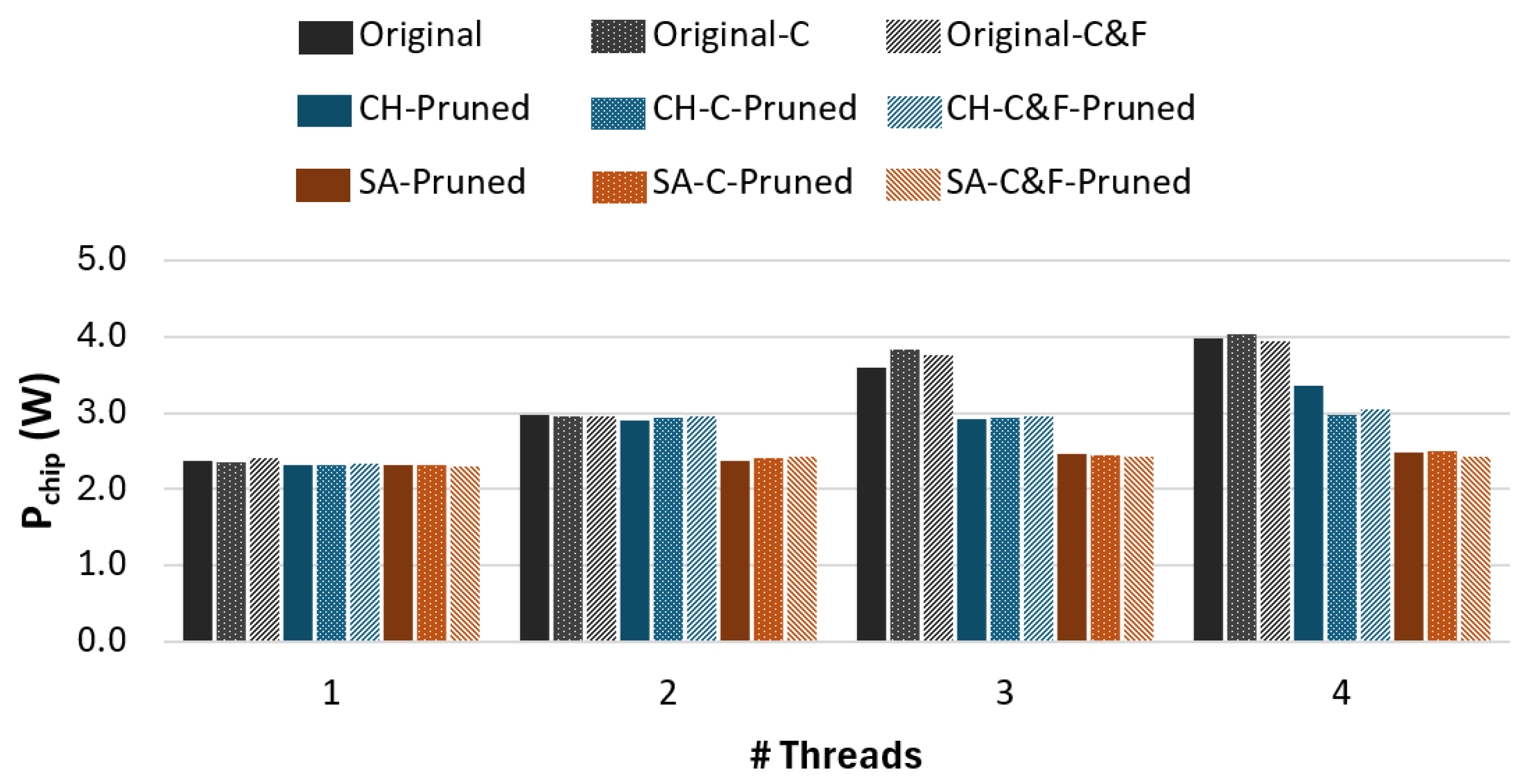
4.3. CPU-Based Implementation

Table 8. Average inference time for various models executed on Raspberry Pi 5 using LCE.

Model	Average Inference Time (µs)
	1 Thread	2 Threads	3 Threads	4 Threads
Original	204	181	159	225
Original-C	197	177	154	222
Original-C&F	222	200	182	254
CH-Pruned	160	130	125	127
CH-C-Pruned	153	127	131	127
CH-C&F-Pruned	163	137	141	138
SA-Pruned	129	114	109	107
SA-C-Pruned	124	112	107	112
SA-C&F-Pruned	136	122	117	129

presents the average inference time over 10,000 runs for each model, evaluated using different numbers of threads on the Raspberry Pi 5. As observed, multi-threaded processing did not result in a linear performance improvement. The fastest inference speed for each model is highlighted in bold. Moreover, most models reached a performance plateau when using 2 or 3 threads. This is likely due to the small size of the BNN-based IDSs, where the overheads associated with multi-threaded execution, such as inefficient load distribution and memory access bottlenecks, outweigh the benefits of parallel processing.

When comparing the original model (“Original”) with the pruned models (“CH-Pruned” and “SA-Pruned”), the pruned models achieved speedups of 1.25× for the CH dataset and 1.48× for the SA dataset when run with the optimal number of threads. To align with the LCE optimisation guide [39], all fully-connected layers were replaced with 1 × 1 convolutional layers. Surprisingly, the Coarse model’s inference time is nearly identical to that of the full model, despite containing fewer convolutional layers. This is likely because the Coarse model, which has two fully-connected layers replaced with two 1 × 1 convolutional layers, is still not fully optimised, limiting its performance. Consequently, since running the Coarse model does not improve inference speed, the C2F implementation is not recommended for CPU-based IDS. Instead, the original (“Original”) or pruned models (“CH-Pruned” and “SA-Pruned”) should be used.

To measure power consumption, the power monitoring facility of the Raspberry Pi 5 is utilised. Specifically, during multiple runs of model inference, the command vcgencmd pmic_read_adc is used to retrieve the voltage and current of the SoC’s internal core, which includes both the CPU and GPU. The average power consumption of the SoC core, denoted as $P_{chip}$, is calculated from these voltage and current values and is used to make relative comparisons among the models and executions with different numbers of threads, as shown in Figure 7. Considering the optimal number of threads for the best inference speed, the pruned models for the CH and SA datasets (“CH-Pruned” and “SA-Pruned”) with 3 and 4 threads, respectively, achieve power-consumption reductions of approximately 20% and 30% compared to the original model (“Original”) with 3 threads.

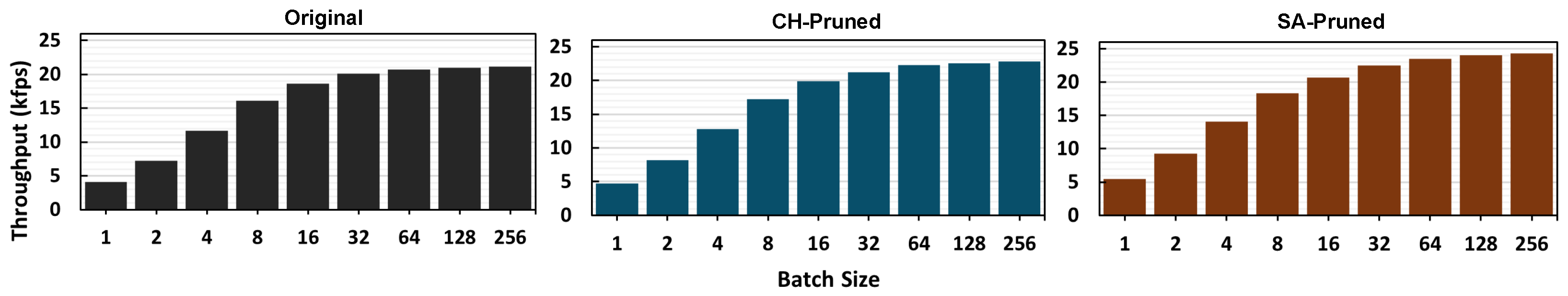
4.4. GPU-Based Implementation

Table 9. Average inference time for various models executed on Jetson Orin Nano using BTC.

Model	Average Inference Time (µs)
	7 W Mode	15 W Mode
Original	512	243
Original-C	413	178
Original-C&F	529	254
CH-Pruned	424	212
CH-C-Pruned	357	170
CH-C&F-Pruned	458	235
SA-Pruned	369	183
SA-C-Pruned	305	140
SA-C&F-Pruned	405	205

presents the average inference time for each model with a batch size of 1, measured over 10,000 runs on the Jetson Orin Nano GPU. The models were evaluated in two power modes: “7 W” and “15 W,” corresponding to GPU clock speeds of 408 MHz and 625 MHz, respectively.

The pruned models without the C2F structure (“CH-Pruned” and “SA-Pruned”) achieve speedups of 1.2× and 1.4× in ‘7 W’ mode and 1.1× and 1.3× in “15 W” mode, respectively, compared to the original model (“Original”). The Coarse model (highlighted in bold) reduces inference time by 19.3%, 15.8%, and 17.3% for the original, pruned CH, and pruned SA models, respectively, in “7 W” mode, compared to running their corresponding full models. These savings slightly increase in “15 W” mode, with reductions of 26.7%, 19.8%, and 23.5%, respectively. In cases where an attack is detected, the additional inference time required for the Fine model leads to a slight increase in total execution time for the “Original-C&F”, “CH-C&F-Pruned”, and “SA-C&F-Pruned” models. The increases are 3.3%, 8.0%, and 9.8% in “7 W” mode, and 4.3%, 10.8%, and 10.7% in “15 W” mode, respectively. However, this additional processing time is considered minimal, as most of the time a vehicle network operates in a normal state.

The relatively low inference speed of the GPU may be due to the underutilisation of its hardware tensor cores. To investigate this, batch sizes were varied from 1 to 256, as shown in Figure 8. With a batch size of 256, the throughput of the “Original” model reaches approximately 21 kfps, which is more than 5× faster than with a batch size of 1. Similarly, for “CH-Pruned” and “SA-Pruned”, a batch size of 256 achieves a similar speedup of about 5×, reaching approximately 23 kfps and 24 kfps, respectively. However, large batch sizes are unsuitable for an IDS application that requires real-time inference, as they introduce significant detection delays and may slow down threat response time. Therefore, for further comparisons, inference time with a batch size of 1 will be used.

The system monitoring utility on the Jetson Orin Nano is used to approximate the GPU’s power consumption for relative comparison. The command tegrastats is issued during multiple runs of model infernece to obtain the average power consumption of the GPU, CPU, and computer-vision accelerators via the power rail named “VDD_CPU_GPU_CV”, which is referred to as $P_{chip}$ in Figure 9. As shown, the $P_{chip}$ of the original model remains below 1.2 W in “7 W” mode and below 2.7 W in “15 W” mode, with a slight reduction observed for the pruned models in both cases. This indicates that pruning not only improves inference speed but also results in minor power savings in GPU-based implementations.

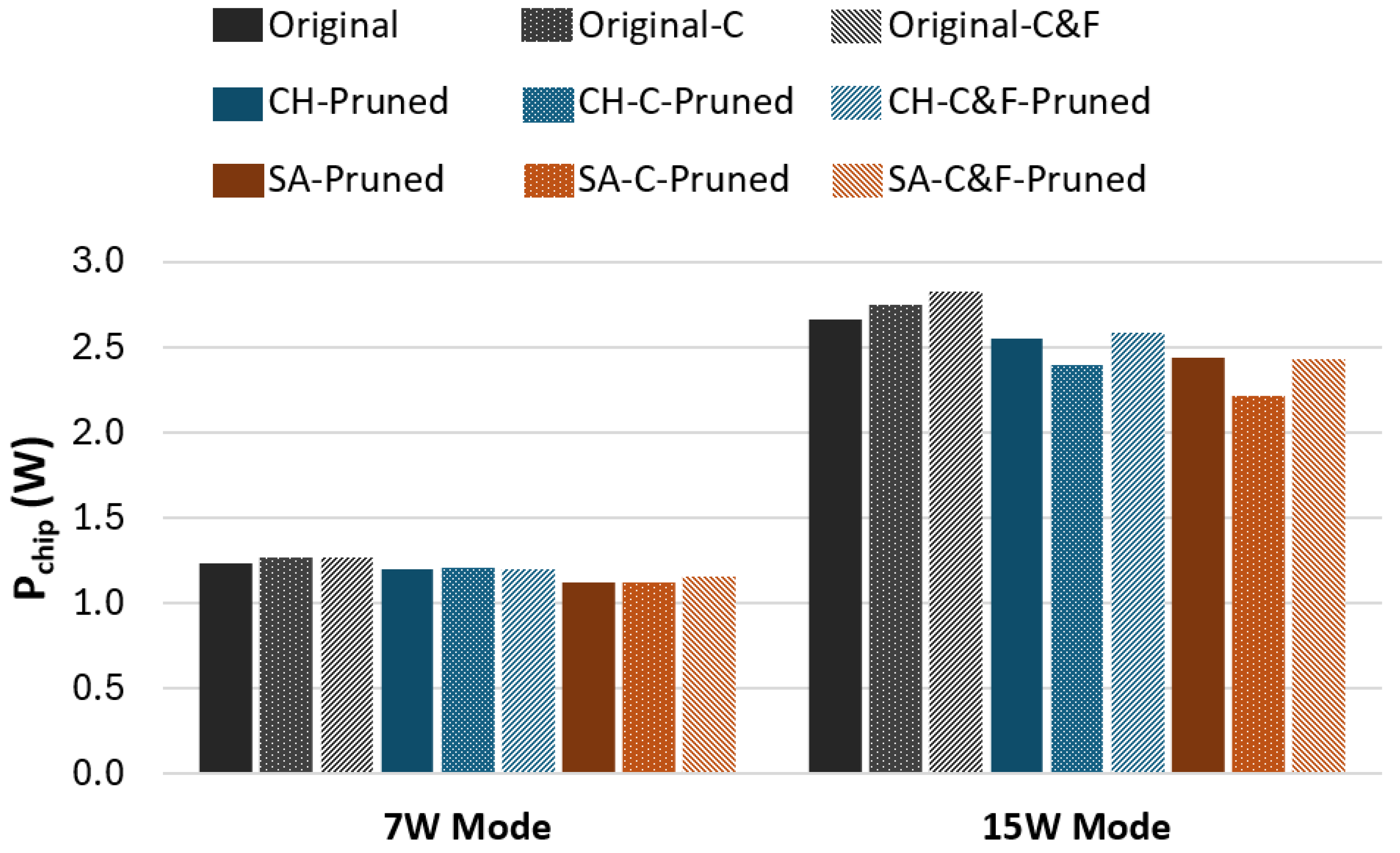
4.5. FPGA-Based Implementation

The FPGA-based hardware implementation is based on the work in [16], designed for the Zynq SoC on the Zedboard. As shown in Figure 10, the system consists of two main components: the Processing System (PS) and the Programmable Logic (PL), also known as the FPGA. The BNN inference process primarily takes place on the FPGA, where design blocks are generated using the FINN compiler. These blocks include Shared Layers, the Coarse Model Head, and the Fine Model block. The process starts with the AXI DMA [50], which retrieves a CAN image from the DDR3 memory and feeds it into the Shared Layers, consisting of Conv1 to Conv3. The AXIS Broadcaster [51] then duplicates the output of Conv3, sending one copy to the Coarse Model Head and the other to the Fine Model. The Model Interpreter, a custom block developed in Verilog, determines whether the Fine Model’s result is required based on the Coarse Model Head’s output. If the Coarse Model Head classifies the input as normal, the Model Interpreter issues a reset signal (FMReset) to the Fine Model, allowing the next inference process to begin. However, if an attack is detected, the Model Interpreter waits for the Fine Model’s output to classify the specific attack type.

Table 10. Resource utilisation and power consumption of FPGA-based implementations.

Model	LUTs	BRAM	Pchip (W)	Inf. Time (µs)
Original	24,463	3.29 Mb	2.41	65
Original-C2F	26,793	4.52 Mb	2.51	53 (Coarse) 65 (C&F)
CH-Pruned	13,613	1.35 Mb	2.13	63
CH-C2F-Pruned	14,557	1.48 Mb	2.13	42 (Coarse) 63 (C&F)
SA-Pruned	10,067	0.67 Mb	1.89	60
SA-C2F-Pruned	10,909	0.74 Mb	1.89	40 (Coarse) 60 (C&F)

presents the results of the FPGA-based implementations. Since the unknown attack head is not included in this work, FINN can generate a design with higher parallelism, which results in inference times of 65 µs, 63 µs, and 60 µs at a clock speed of 100 MHz for the original (“Original”) and pruned models (“CH-Pruned” and “SA-Pruned”), respectively. Running the Coarse model instead of the full model reduces inference time by 18% for the original (“Original”) model and 33% for both pruned (“CH-Pruned” and “SA-Pruned”) models. Furthermore, since the Coarse and Fine models run in parallel, executing both models does not negatively impact inference speed, achieving the same performance as running their corresponding full models.

In terms of resource utilisation, pruning significantly reduces LUT and BRAM usage compared to the original model implementation, by 44% and 59% for the CH dataset, and 59% and 80% for the SA dataset, respectively. Additionally, Vivado’s estimated power consumption ($P_{chip}$), shown in Table 10, indicates that the pruned models consume 12% and 22% less power for the CH and SA datasets, respectively. Implementing the C2F approach increases LUT and BRAM usage by 10% and 37% for the original model. However, for the pruned CH and SA models, the additional resource overhead is minimal, requiring only 7% and 9% more LUTs and 8% and 10% more BRAM, respectively. This is primarily because pruning significantly reduces intermediate activations, and introducing two fully connected layers for the Coarse model requires relatively few resources and minimal computational effort. The minimal resource utilisation of our IDS, particularly without requiring any DSPs, leaves sufficient remaining capacity for co-deployment with other computation-intensive tasks, such as real-time video processing, on the same FPGA SoC.

4.6. Performance and Energy Efficiency Comparison

The power consumption of each platform, measured using a power meter referred to as $P_{board}$, is also recorded for further comparison. Measuring the power of the entire system ensures that all components involved, such as memory, are accounted for during inference. As shown in

Table 11. Energy efficiency comparison of BNN-based IDSs across different platforms.

Model	FPGA			GPU (Max Performance)			CPU (Max Performance)
	Inf. Time (µs)	Pboard (W)	Efficiency (# Inf./J)	Inf. Time (µs)	Pboard (W)	Efficiency (# Inf./J)	Inf. Time (µs)	Pboard (W)	Efficiency (# Inf./J)
Original	65	4.6	3344	243	9.1	452	159	7.2	873
Original-C	53	4.7	4014	178	9.1	617	154	7.2	902
Original-C&F	65	4.7	3273	254	9.2	428	182	7.2	763
CH-Pruned	63	4.5	3527	212	9.0	524	125	6.3	1270
CH-C-Pruned	42	4.4	5291	175	8.9	642	127	6.3	1250
CH-C&F-Pruned	63	4.5	3527	240	9.0	463	137	6.3	1159
SA-Pruned	60	4.5	3788	183	8.8	621	107	5.8	1611
SA-C-Pruned	40	4.4	5682	145	8.7	793	107	5.7	1640
SA-C&F-Pruned	60	4.4	3788	210	8.9	535	117	5.6	1526

, the FPGA platform has the lowest $P_{board}$, ranging from 4.4 to 4.7 W. In contrast, the GPU, operating in its maximum performance mode (“15W”), consumes approximately 9 W, while the CPU, running at its optimal thread count, consumes between 5.6 W to 7.2 W. Notably, for the CPU implementation, pruning the models results in a 12% reduction in power consumption for the CH dataset and a 19% reduction for the SA dataset.

In terms of inference time, the FPGA implementations also consistently outperforms both GPU and CPU implementations. For the original model, the FPGA is 3.7× faster than the GPU and 2.4× faster than the CPU. For the pruned models, the FPGA achieves a 3.6× speedup over the GPU and a 2.0× speedup over the CPU for the CH dataset. Similarly, for the SA dataset, the FPGA outperforms the GPU by 3.0× and the CPU by 1.8×. Unlike the GPU and CPU, whose inference time increases when both the Coarse and Fine models (C&F) run sequentially, the FPGA implementation maintains its speed due to parallel execution. As a result, the FPGA’s speedup advantage over the CPU and GPU slightly increases when both models are required to run.

The number of inferences per joule is used to measure energy efficiency and is calculated as $E={\displaystyle \frac{1}{P\times T}}$, where E represents energy efficiency (inferences per joule), P is the average power consumption in watts (W), and T is the average inference time in seconds (s). As shown in Table 11, the FPGA implementations achieve the highest energy efficiency, followed by the CPU, while the GPU demonstrates the lowest efficiency. As previously mentioned, the low energy efficiency of the GPU can be attributed to the underutilisation of its hardware due to smaller batch sizes. The FPGA implementation is 7.4× more energy efficient than the GPU and 3.8× more energy efficient than the CPU for the original model without pruning. For the pruned models, the FPGA achieves a 6.7× improvement over the GPU and a 2.8× improvement over the CPU for the CH dataset, while for the SA dataset, it is superior to the GPU by 6.1× and the CPU by 2.3×.

Regarding the C2F approach, the energy efficiency of the FPGA implementation executing both the Coarse and Fine models (C&F) remains nearly identical to that of the original model, as inference times are the same and the power consumption only varies slightly. However, for the GPU deployment, energy efficiency consistently decreases when running both Coarse and Fine models (C&F) compared to running the original model. Although the C2F approach is included for CPU-based implementations in Table 11, it is not recommended for real applications, as running the Coarse model alone does not improve inference time, as previously discussed.

The superior efficiency of implementing BNN models on FPGAs comes from their architectural flexibility. Unlike CPUs and GPUs, which are based on fixed hardware architectures, FPGAs offer reconfigurable resources, such as LUTs and BRAMs, that can be customised to match the structure of any BNN. Moreover, the XNOR and popcount operations used in BNNs can be naturally and efficiently mapped onto FPGA fabric using its native logic resources. In contrast, CPUs may struggle to execute these bit operations efficiently due to their limited support in standard instruction sets. Similarly, while GPUs generally offer high throughput, they are optimised for parallel processing with floating-point operations and often require large batch sizes to achieve optimal hardware utilisation.

4.7. A Comparative Performance Analysis of the Proposed FPGA-Based IDS Against Other BNN-Based Solutions

Table 12. Performance comparison of our FPGA-based implementation with other BNN-based IDS solutions.

Model	Dataset	Accuracy (%)	F1 (%)	Avg. Inf. Time (µs)	Device
BNN-FC [13]	4 Cars	93.15	-	400	Xilinx PYNQ Artix-7
BCNN [14]		95.51	96.93	600	Nvidia RTX 2070 Super
BNN-C2F [15]	CH	99.83	99.75	364	Zedboard
BIDS [16]		99.72	99.52	169
Proposed IDS		99.92	99.91	50
BIDS [16]	SA	98.87	95.54	162
Proposed IDS		99.96	99.91	48
Proposed IDS	ATK&DEF	96.96	94.21	56

compares the FPGA implementations of C2F-based models with other BNN-based IDSs. The F1 scores are averaged across available attacks for simplified comparison. Notably, the works from [13,14] use their own datasets, collected from four different vehicles on a fixed route. Additionally, BIDS [16] considers DoS attacks as unknown, excluding them from its training set. Since the inference time of the C2F approach varies depending on the input, an average value is calculated. Normal CAN images are processed only by the Coarse model, while attack images require the execution of the Fine model to classify the specific attack type. Therefore, the average inference time is estimated based on the label distribution of the dataset. As observed in Table 3, for the CH dataset, 63% of the data are normal and 37% are labeled as attack. Using this distribution, the average inference time is about (63% × 42 µs + 37% × 63 µs) / 100% ≈ 50 µs. Similarly, for the SA dataset, with 62% normal and 38% attack images, the average inference time is approximately (62% × 40 µs + 38% × 60 µs) / 100% ≈ 48 µs. For the ATK&DEF dataset, which uses the original model and has 71% normal and 29% attack samples, the average inference time can be calculated as (71% × 53 µs + 29% × 65 µs) / 100% ≈ 56 µs. This same calculation method is applied to the raw data from the previous C2F work [15] to determine the average inference time. The results show that the pruned models developed in this work outperform previous studies in both accuracy and inference time.

Our IDS achieves an average inference time ranging from 48 to 56 µs, making it approximately 8× faster than BNN-FC [13] and 12× faster than BCNN [14]. Using a comparable dataset, the pruned model implementation is approximately 7.2× and 3.3× faster than BNN-C2F [15] and BIDS [16], respectively. In terms of effectiveness, the proposed IDS outperforms existing methods in both accuracy and average F1 score across all datasets. For the CH dataset, our IDS achieves 0.09% higher accuracy and 0.16% higher F1 score compared to BNN-C2F, and improvements of 0.20% and 0.39% over BIDS, respectively. The superiority is even more noticeable for the SA dataset, where our model achieves 1.09% higher accuracy and 4.37% higher average F1 score compared to BIDS. This improvement for the SA dataset, which has limited data, can be partly attributed to the use of a sliding-window technique, which significantly increases the number of encoded CAN images. It is also worth noting that BIDS supports unknown attack detection, which may slightly compromise its overall classification accuracy.

5. Conclusions

This paper investigates further optimisation of BNN-based IDSs through network pruning and compares their implementation on CPU, GPU and FPGA in terms of inference time and power consumption. The sliding-window technique is utilised during data-encoding process to enhance data availability. In experiments across three datasets, this technique can improve the model accuracy by up to 0.66%. Cosine similarity between real-valued and binarised weights is used as the pruning metric. The pruning process consists of three steps: running pruning sensitivity analysis, removing filters or channels based on a 90% accuracy threshold, and fine-tuning the pruned model.

The experimental results show that, across three datasets, models trained on two of them achieve up to a 91.07% parameter reduction with only a 0.01% accuracy drop. Additionally, the pruned models are restructured into a Coarse-to-Fine (C2F) approach, where the Coarse model, containing fewer convolutional layers, performs initial attack detection, and the Fine model is executed only when an attack is detected to classify its type. All models, including the original, pruned, and C2F-based versions, are deployed on CPU, GPU, and FPGA using state-of-the-art frameworks for comparison.

The deployment results demonstrate that FPGA, with its ability to run the Coarse and Fine models in parallel, delivers the fastest inference and the highest energy efficiency. For the original model, the FPGA implementation achieves an inference speed of 65 µs, making it faster than GPU by 3.7× and the CPU by 2.4×, while being 7.4× more energy efficient than the GPU and 3.8× more efficient than the CPU. For the pruned models, the FPGA maintains a significant advantage, achieving up to 3.6× speed and 6.7× energy efficiency over the GPU, and 2.0× speed and 2.8× energy efficiency over the CPU. Additionally, the C2F approach on FPGA achieves the fastest average inference time among BNN-based IDSs while maintaining high accuracy.

A key limitation of the developed IDS is that its based on supervised learning, which makes it less effective in detecting unknown or stealthy attacks that closely mimic normal CAN ID patterns. Moreover, while the C2F approach helps reduce inference time, since only the lightweight Coarse model is active during normal operation, it comes at the cost of slightly reduced overall accuracy. To address these issues, future work will explore the integration of an unsupervised learning head into the Coarse model to enable the detection of unknown attacks. Additionally, we plan to investigate mixed-precision IDS architectures. In particular, the Coarse model, which is critical for initial attack detection, will be implemented using higher bit precision (e.g., 2-bit or 4-bit), while the Fine model may continue to operate at 1-bit precision to retain efficiency.

References

1. Kang, T.U.; Song, H.M.; Jeong, S.; Kim, H.K. Automated reverse engineering and attack for CAN using OBD-II. In Proceedings of the 2018 IEEE 88th Vehicular Technology Conference (VTC-Fall), Chicago, IL, USA, 27–30 August 2018; IEEE: Piscatway, NJ, USA, 2018; pp. 1–7. [Google Scholar]
2. Miller, C. Remote exploitation of an unaltered passenger vehicle. In Proceedings of the Black Hat USA, Las Vegas, NV, USA, 1–6 August 2015. [Google Scholar]
3. Jafarnejad, S.; Codeca, L.; Bronzi, W.; Frank, R.; Engel, T. A car hacking experiment: When connectivity meets vulnerability. In Proceedings of the 2015 IEEE globecom Workshops (GC Wkshps), San Diego, CA, USA, 6–10 December 2015; IEEE: Piscatway, NJ, USA, 2015; pp. 1–6. [Google Scholar]
4. Aliwa, E.; Rana, O.; Perera, C.; Burnap, P. Cyberattacks and countermeasures for in-vehicle networks. ACM Comput. Surv. (CSUR) 2021, 54, 1–37. [Google Scholar] [CrossRef]
5. Van Herrewege, A.; Singelee, D.; Verbauwhede, I. CANAuth-a simple, backward compatible broadcast authentication protocol for CAN bus. In Proceedings of the ECRYPT Workshop on Lightweight Cryptography, Louvain-la-Neuve, Belgium, 28 November 2011; Volume 2011, p. 20. [Google Scholar]
6. Hazem, A.; Fahmy, H. Lcap-a lightweight can authentication protocol for securing in-vehicle networks. In Proceedings of the 10th Escar Embedded Security in Cars Conference, Berlin, Germany, 28–29 November 2012; Volume 6, p. 172. [Google Scholar]
7. Farag, W.A. CANTrack: Enhancing automotive CAN bus security using intuitive encryption algorithms. In Proceedings of the 2017 7th International Conference on Modeling, Simulation, and Applied Optimization (ICMSAO), Sharjah, United Arab Emirates, 4–6 April 2017; IEEE: Piscatway, NJ, USA, 2017; pp. 1–5. [Google Scholar]
8. Lokman, S.F.; Othman, A.T.; Abu-Bakar, M.H. Intrusion detection system for automotive Controller Area Network (CAN) bus system: A review. EURASIP J. Wirel. Commun. Netw. 2019, 2019, 1–17. [Google Scholar] [CrossRef]
9. Rajapaksha, S.; Kalutarage, H.; Al-Kadri, M.O.; Petrovski, A.; Madzudzo, G.; Cheah, M. AI-based intrusion detection systems for in-vehicle networks: A survey. ACM Comput. Surv. 2023, 55, 1–40. [Google Scholar] [CrossRef]
10. Khandelwal, S.; Shreejith, S. A lightweight FPGA-based IDS-ECU architecture for automotive CAN. In Proceedings of the 2022 International Conference on Field-Programmable Technology (ICFPT), Hong Kong, China, 5–9 December 2022; IEEE: Piscatway, NJ, USA, 2022; pp. 1–9. [Google Scholar]
11. Khandelwal, S.; Walsh, A.; Shreejith, S. Quantised Neural Network Accelerators for Low-Power IDS in Automotive Networks. In Proceedings of the 2023 Design, Automation & Test in Europe Conference & Exhibition (DATE), Antwerp, Belgium, 17–19 April 2023; IEEE: Piscatway, NJ, USA, 2023; pp. 1–2. [Google Scholar]
12. Courbariaux, M.; Hubara, I.; Soudry, D.; El-Yaniv, R.; Bengio, Y. Binarized neural networks: Training deep neural networks with weights and activations constrained to +1 or −1. arXiv 2016, arXiv:1602.02830. [Google Scholar]
13. Zhang, L.; Yan, X.; Ma, D. A binarized neural network approach to accelerate in-vehicle network intrusion detection. IEEE Access 2022, 10, 123505–123520. [Google Scholar] [CrossRef]
14. Zhang, L.; Yan, X.; Ma, D. Efficient and Effective In-Vehicle Intrusion Detection System using Binarized Convolutional Neural Network. In Proceedings of the IEEE INFOCOM 2024-IEEE Conference on Computer Communications, Vancouver, BC, Canada, 20–23 May 2024; IEEE: Piscatway, NJ, USA, 2024; pp. 2299–2307. [Google Scholar]
15. Rangsikunpum, A.; Amiri, S.; Ost, L. An FPGA-Based Intrusion Detection System Using Binarised Neural Network for CAN Bus Systems. In Proceedings of the 2024 IEEE International Conference on Industrial Technology (ICIT), Bristol, UK, 25–27 March 2024; IEEE: Piscatway, NJ, USA, 2024; pp. 1–6. [Google Scholar]
16. Rangsikunpum, A.; Amiri, S.; Ost, L. BIDS: An efficient Intrusion Detection System for in-vehicle networks using a two-stage Binarised Neural Network on low-cost FPGA. J. Syst. Archit. 2024, 156, 103285. [Google Scholar] [CrossRef]
17. Rangsikunpum, A.; Amiri, S.; Ost, L. A Reconfigurable Coarse-to-Fine Approach for the Execution of CNN Inference Models in Low-Power Edge Devices. IET Comput. Digit. Tech. 2024, 2024, 6214436. [Google Scholar] [CrossRef]
18. Seo, E.; Song, H.M.; Kim, H.K. GIDS: GAN based intrusion detection system for in-vehicle network. In Proceedings of the 2018 16th Annual Conference on Privacy, Security and Trust (PST), Belfast, UK, 28–30 August 2018; IEEE: Piscatway, NJ, USA, 2018; pp. 1–6. [Google Scholar]
19. Han, M.L.; Kwak, B.I.; Kim, H.K. Anomaly intrusion detection method for vehicular networks based on survival analysis. Veh. Commun. 2018, 14, 52–63. [Google Scholar] [CrossRef]
20. Kang, H.; Kwak, B.I.; Lee, Y.H.; Lee, H.; Lee, H.; Kim, H.K. Car hacking and defense competition on in-vehicle network. In Proceedings of the Workshop on Automotive and Autonomous Vehicle Security (AutoSec), Online, 25 February 2021; Volume 2021, p. 25. [Google Scholar]
21. Ioffe, S. Batch normalization: Accelerating deep network training by reducing internal covariate shift. arXiv 2015, arXiv:1502.03167. [Google Scholar]
22. Hinton, G. Improving neural networks by preventing co-adaptation of feature detectors. arXiv 2012, arXiv:1207.0580. [Google Scholar]
23. Sharma, A.; Vans, E.; Shigemizu, D.; Boroevich, K.A.; Tsunoda, T. DeepInsight: A methodology to transform a non-image data to an image for convolution neural network architecture. Sci. Rep. 2019, 9, 11399. [Google Scholar] [CrossRef] [PubMed]
24. Zhao, Q.; Chen, M.; Gu, Z.; Luan, S.; Zeng, H.; Chakrabory, S. CAN bus intrusion detection based on auxiliary classifier GAN and out-of-distribution detection. ACM Trans. Embed. Comput. Syst. (TECS) 2022, 21, 45. [Google Scholar] [CrossRef]
25. Mao, H.; Han, S.; Pool, J.; Li, W.; Liu, X.; Wang, Y.; Dally, W.J. Exploring the granularity of sparsity in convolutional neural networks. In Proceedings of the IEEE Conference on Computer Vision and Pattern Recognition Workshops, Honolulu, HI, USA, 21–26 July 2017; pp. 13–20. [Google Scholar]
26. Han, S.; Pool, J.; Tran, J.; Dally, W. Learning both weights and connections for efficient neural network. Adv. Neural Inf. Process. Syst. 2015, 28, 1–9. [Google Scholar]
27. Hu, H. Network trimming: A data-driven neuron pruning approach towards efficient deep architectures. arXiv 2016, arXiv:1607.03250. [Google Scholar]
28. Han, S.; Liu, X.; Mao, H.; Pu, J.; Pedram, A.; Horowitz, M.A.; Dally, W.J. EIE: Efficient inference engine on compressed deep neural network. ACM SIGARCH Comput. Archit. News 2016, 44, 243–254. [Google Scholar] [CrossRef]
29. Luo, J.H.; Wu, J. An entropy-based pruning method for cnn compression. arXiv 2017, arXiv:1706.05791. [Google Scholar]
30. He, Y.; Zhang, X.; Sun, J. Channel pruning for accelerating very deep neural networks. In Proceedings of the IEEE International Conference on Computer Vision, Venice, Italy, 22–29 October 2017; pp. 1389–1397. [Google Scholar]
31. Li, Y.; Ren, F. Bnn pruning: Pruning binary neural network guided by weight flipping frequency. In Proceedings of the 2020 21st International Symposium on Quality Electronic Design (ISQED), Santa Clara, CA, USA, 25–26 March 2020; IEEE: Piscatway, NJ, USA, 2020; pp. 306–311. [Google Scholar]
32. Guerra, L.; Drummond, T. Automatic pruning for quantized neural networks. In Proceedings of the 2021 Digital Image Computing: Techniques and Applications (DICTA), Gold Coast, Australia, 29 November–1 December 2021; IEEE: Piscatway, NJ, USA, 2021; pp. 01–08. [Google Scholar]
33. Bannink, T.; Hillier, A.; Geiger, L.; de Bruin, T.; Overweel, L.; Neeven, J.; Helwegen, K. Larq compute engine: Design, benchmark and deploy state-of-the-art binarized neural networks. Proc. Mach. Learn. Syst. 2021, 3, 680–695. [Google Scholar]
34. Chen, T.; Moreau, T.; Jiang, Z.; Zheng, L.; Yan, E.; Shen, H.; Cowan, M.; Wang, L.; Hu, Y.; Ceze, L.; et al. {TVM}: An automated {End-to-End} optimizing compiler for deep learning. In Proceedings of the 13th USENIX Symposium on Operating Systems Design and Implementation (OSDI 18), Carlsbad, CA, USA, 10–12 July 2018; pp. 578–594. [Google Scholar]
35. Zhang, J.; Pan, Y.; Yao, T.; Zhao, H.; Mei, T. dabnn: A super fast inference framework for binary neural networks on arm devices. In Proceedings of the 27th ACM International Conference on Multimedia, Nice, France, 21–25 October 2019; pp. 2272–2275. [Google Scholar]
36. Google. LiteRT. Available online: https://ai.google.dev/edge/litert (accessed on 27 February 2025).
37. Geiger, L.; Team, P. Larq: An open-source library for training binarized neural networks. J. Open Source Softw. 2020, 5, 1746. [Google Scholar] [CrossRef]
38. Abadi, M.; Agarwal, A.; Barham, P.; Brevdo, E.; Chen, Z.; Citro, C.; Corrado, G.S.; Davis, A.; Dean, J.; Devin, M.; et al. TensorFlow: Large-Scale Machine Learning on Heterogeneous Systems. Available online: https://www.tensorflow.org/ (accessed on 27 February 2025).
39. Larq. Optimizing Models for Larq Compute Engine. Available online: https://docs.larq.dev/compute-engine/model_optimization_guide/ (accessed on 27 February 2025).
40. Li, A.; Su, S. Accelerating binarized neural networks via bit-tensor-cores in turing gpus. IEEE Trans. Parallel Distrib. Syst. 2020, 32, 1878–1891. [Google Scholar] [CrossRef]
41. NVIDIA. NVIDIA Tensor Cores. Available online: https://www.nvidia.com/en-eu/data-center/tensorcore/ (accessed on 27 February 2025).
42. Umuroglu, Y.; Fraser, N.J.; Gambardella, G.; Blott, M.; Leong, P.; Jahre, M.; Vissers, K. Finn: A framework for fast, scalable binarized neural network inference. In Proceedings of the 2017 ACM/SIGDA International Symposium on Field-Programmable Gate Arrays, Monterey, CA, USA, 22–24 February 2017; pp. 65–74. [Google Scholar]
43. Blott, M.; Preußer, T.B.; Fraser, N.J.; Gambardella, G.; O’brien, K.; Umuroglu, Y.; Leeser, M.; Vissers, K. FINN-R: An end-to-end deep-learning framework for fast exploration of quantized neural networks. ACM Trans. Reconfigurable Technol. Syst. (TRETS) 2018, 11, 1–23. [Google Scholar] [CrossRef]
44. Pappalardo, A. Xilinx/brevitas; Zenodo: Geneva, Switzerland, 2023. [Google Scholar] [CrossRef]
45. ARM. AMBA AXI-Stream Protocol Specification; ARM: Cambridge, UK, 2021. [Google Scholar]
46. Paszke, A.; Gross, S.; Chintala, S.; Chanan, G.; Yang, E.; DeVito, Z.; Lin, Z.; Desmaison, A.; Antiga, L.; Lerer, A. Automatic Differentiation in PyTorch. In Proceedings of the 2017 Neural Information Processing Systems, Long Beach, CA, USA, 4–9 December 2017. [Google Scholar]
47. Raspberry Pi. Raspberry Pi 5. Available online: https://www.raspberrypi.com/products/raspberry-pi-5/ (accessed on 27 February 2025).
48. NVIDIA. Jetson Orin Nano Super Developer Kit. Available online: https://www.nvidia.com/en-gb/autonomous-machines/embedded-systems/jetson-orin/nano-super-developer-kit/ (accessed on 27 February 2025).
49. Avnet. Zedboard—Avnet Boards. Available online: https://www.avnet.com/wps/portal/us/products/avnet-boards/avnet-board-families/zedboard/ (accessed on 27 February 2025).
50. AMD. AXI DMA LogiCORE IP Product Guide (PG021). Available online: https://docs.amd.com/r/en-US/pg021_axi_dma (accessed on 27 February 2025).
51. AMD. AXI4-Stream Infrastructure IP Suite (PG085). Available online: https://docs.amd.com/r/en-US/pg085-axi4stream-infrastructure/AXI4-Stream-Broadcaster (accessed on 27 February 2025).
Figure 1. Vehicle network CAN Bus: (a) Layout of a CAN message. (b) Vulnerability exploited by an attacker via an access point.
Electronics 14 01710 g001
Figure 2. Development process of the proposed BNN-based IDSs: (1) training the original model; (2) performing channel pruning on convolutional layers; and (3) constructing and fine-tuning the Coarse-to-Fine model based on the pruned model.
Electronics 14 01710 g002
Figure 3. Pre-processing for the proposed IDS input: (a) utilising one-hot-vector encoding; (b) implementing a sliding window (SW) with a shifting value of 2 to form CAN images.
Electronics 14 01710 g003
Figure 4. Pruning method: (a) the three steps of the pruning process; (b) filter pruning to reduce the number of activation channels in layer i.
Electronics 14 01710 g004
Figure 5. Pruning sensitivity in the first iteration of the pruning process across three datasets.
Electronics 14 01710 g005
Figure 6. The execution of the C2F-based IDS in this work: (a) sequential execution on GPU and CPU, and (b) parallel execution on FPGA, where t C and t F denote the times at which the Coarse and Fine models produce their results, respectively.
Electronics 14 01710 g006
Figure 7. The power consumption of the SoC core ( P c h i p ) on the Raspberry Pi 5 during the execution of various models.
Electronics 14 01710 g007
Figure 8. Throughput of different models with varying batch sizes on the Jetson Orin Nano.
Electronics 14 01710 g008
Figure 9. The power consumption of the GPU, CPU and computer-vision accelerators ( P c h i p ) on the Jetson Orin Nano during the execution of various models.
Electronics 14 01710 g009
Figure 10. FPGA-based hardware implementation for the Zynq SoC on the Zedboard.
Electronics 14 01710 g010