Network Function Placement in Virtualized Radio Access Network with Reinforcement Learning Based on Graph Neural Network

Abstract

In 5G and beyond 5G networks, function placement is a crucial strategy for enhancing the flexibility and efficiency of the Radio Access Network (RAN). However, demonstrating optimal function splitting and placement to meet diverse user demands remains a significant challenge. The function placement problem is known to be NP-hard, and previous studies have attempted to address it using Deep Reinforcement Learning (DRL) approaches. Nevertheless, many existing methods fail to capture the network state in RANs with specific topologies, leading to suboptimal decision-making and resource allocation. In this paper, we propose a method referred to as GDRL, which is a deep reinforcement learning approach that utilizes graph neural networks to address the functional placement problem. To ensure policy stability, we design a policy gradient algorithm called Graph Proximal Policy Optimization (GPPO), which integrates GNNs into both the actor and critic networks. By incorporating both node and edge features, the GDRL enhances feature extraction from the RAN’s nodes and links, providing richer observational data for decision-making and evaluation. This, in turn, enables more accurate and effective decision outcomes. In addition, we formulate the problem as a mixed-integer nonlinear programming model aimed at minimizing the number of active computational nodes while maximizing the centralization level of the virtualized RAN (vRAN). We evaluate the GDRL across different RAN scenarios with varying node configurations. The results demonstrate that our approach achieves superior network centralization and outperforms several existing methods in overall performance.

1. Introduction

The Radio Access Network (RAN) is responsible for providing, coordinating, and managing user device access, serving as a crucial bridge between user equipment and the core network. As a fundamental component of mobile network systems, RAN plays a pivotal role in network performance and efficiency. Consequently, it has a significant impact on infrastructure investments and operational costs for mobile network operators, making it a key area for optimization in mobile network architecture and maintenance.

In legacy RANs, the two main components of a Base Station (BS)—the Remote Radio Unit (RRU) and the Baseband Unit (BBU)—are typically co-located. With the advent of 4 G mobile networks, the Cloud RAN (C-RAN) architecture was introduced to centralize BBUs by deploying them in a central server. In this setup, each RRU connects to its corresponding BBU via a network segment known as the fronthaul network. C-RAN enhances network efficiency by enabling adaptive control based on user mobility, facilitating wireless resource sharing, improving interference management between antennas, and optimizing user data transmission. However, a significant challenge of C-RAN is the high-capacity demand of the fronthaul, which increases deployment costs and pose feasibility issues, especially in large-scale networks with hundreds or thousands of radio units [1].

To mitigate the high costs of C-RAN while preserving its benefits, standardization bodies have developed Next-Generation RAN (NG-RAN) architectures that incorporate softwarization and virtualization RANs [2,3]. The 5G mobile network adopts a software-defined approach, splitting BS functions into three distinct components: Radio Unit (RU), Distributed Unit (DU), and Central Unit (CU). In this setup, only high-layer BS functions are centralized at the CU, while the RU, deployed in a radio hardware unit, handles lower-layer functions and radio frequency processing. The remaining functions are hosted at the DU [4]. These components—RU, DU, CU, and the core network—are interconnected via fronthaul, midhaul, and backhaul interfaces, each with specific capacity and latency requirements. To meet these requirements, 5G RAN introduces functional split options, disaggregating BS functions among the CU, DU and RU [1]. Strategically placing the CU and DU within the network caters the diverse service requirements of user devices, resulting in a significant improvement in RAN flexibility and efficiency [5]. Additionally, standardization bodies promote Network Functions Virtualization (NFV) to increase flexibility and improve resource sharing of infrastructure resources. Virtualizing radio functions and deploy them at optimal locations reduces reliance on specialized hardware, thereby reducing dependence on physical devices and lowering both costs and energy consumption. However, a key challenge is determining the optimal way to split and deploy these Virtualized Network Functions (VNFs) across network nodes while balancing various operational objectives such as minimizing costs, energy consumption, and latency. This challenge is known as the VNF placement problem.

The function placement problem is a combinatorial optimization challenge that involves splitting BS functions, selecting routing paths in the crosshaul transport network, and allocating computational resources among the CU, DU, and RU nodes [6]. In recent years, the rapid development of 5G networks has spurred extensive research on the function placement in vRAN, leading to various approaches, including mathematical optimization techniques (e.g., Mixed-Integer Linear Programming (MILP)) [7,8,9,10,11,12,13,14], heuristic methods [15,16,17,18,19,20,21,22], and Deep Reinforcement Learning (DRL) techniques [23,24,25,26,27,28,29]. However, the function placement problem is NP-hard. While MILP solvers can find optimal solutions, they suffer from slow convergence and high computational complexity making them impractical large-scale networks and real-time applications. Heuristic algorithms can provide satisfactory solutions at a reasonable time but often rely on problem-specific rules, leading to convergence toward local optima rather than global optimum. Deep Reinforcement Learning (DRL) offers an alternative by enhancing performance through iterative experimentation and optimization. In particular, the DRL agent interacts with the RAN environment using a function placement strategy and then continuously optimizes the strategy based on reward values received from the environment, leading to obtainment of the optimal function placement. Compared to exact methods and heuristic approaches, DRL allows real-time management, adapts to traffic and latency constraints, and self-optimize with network variations. Therefore, DRL has become a mainstream approach for addressing the function placement problem. Since function placement is fundamentally a graph optimization problem, many existing DRL methods fail to fully exploit the network’s topological structure, leading to suboptimal strategies. Recent studies have attempted to address this issue by integrating DRL with Graph Neural Networks (GNNs) [28,30,31]. However, traditional GNNs primarily focus on node embedding while neglecting edge attributes. This oversight is significant, as edges in function placement problems carry critical attributes such as bandwidth and latency. Therefore, developing approaches that incorporate both node and edge features is essential for enhancing function placement strategies in complex network environments.

In this paper, we formulate the network function placement problem in vRAN as a mixed integer nonlinear programming model and propose a DRL method based on GNNs, which incorporates both node and edge features to optimize function placement. To solve this problem, we design a Graph Proximal Policy Optimization (GPPO) algorithm, where the actor network integrates GNNs to enhance decision-making, while the GNN-enhanced critic network effectively evaluates actions and estimates value functions. By integrating node and edge features, our approach provides more accurate information for decision-making, making it particularly suitable for graph-based optimization problems where edge attributes play a crucial role. Therefore, our main contributions are as follows:

(1)

We formulate an optimization model using mixed integer nonlinear programming to integrate the functional split and network function placement problems. The objective of the model is to minimize the number of active computing resources while maximizing the centralization level of vRAN. Details can be found in Section 3;

(2)

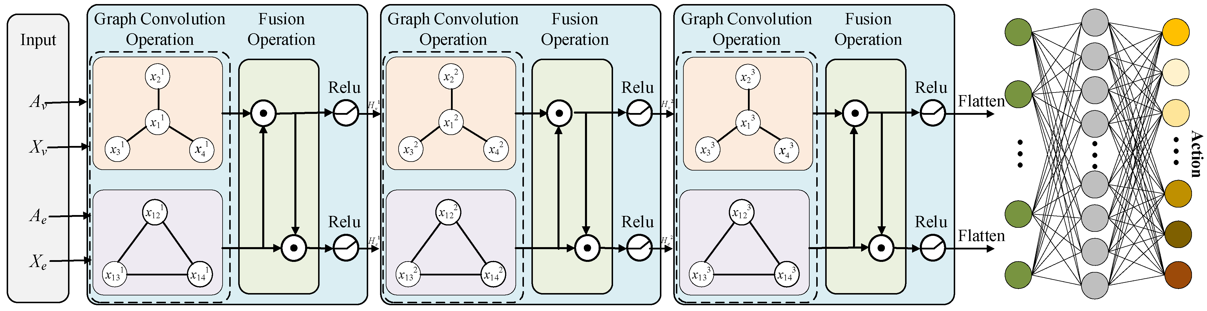
We propose an efficient GPPO-based DRL algorithm. In this framework, GNNs incorporating both node and edge feature embeddings are integrated into the actor and critic networks, providing a more comprehensive view of the network state. This enables the actor network to make more precise policy decisions and the critic network to deliver more accurate evaluations. The improvement is mainly due to the GNN’s ability to effectively leverage topological structure information, enhancing the embedded representation of both node and edge features. Refer to Section 4 for more information;

(3)

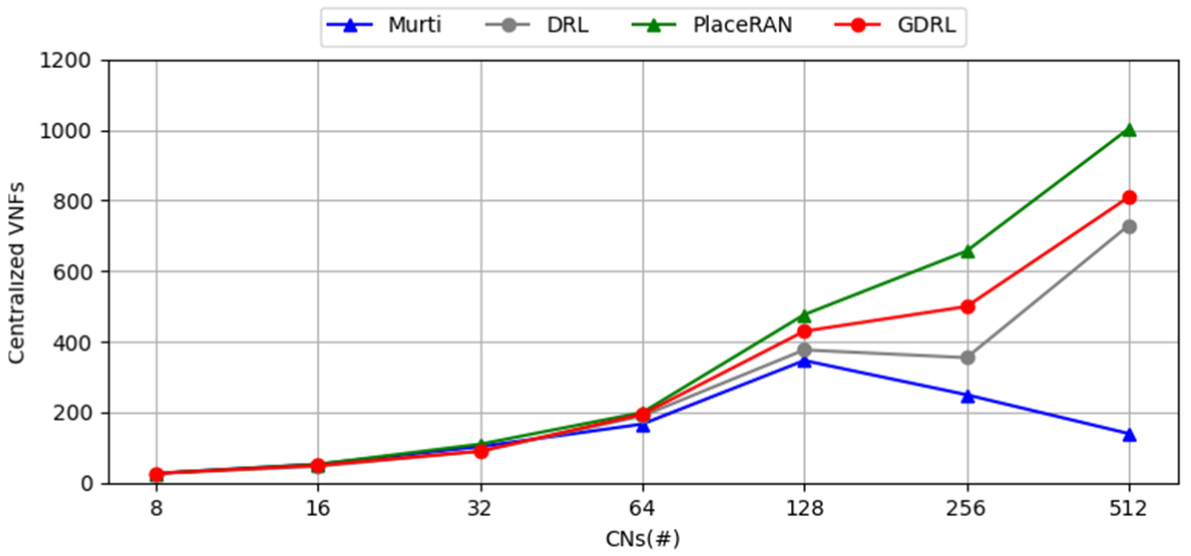
Simulation experiments across different RAN scenarios with varying node configurations demonstrate that our approach achieves a superior network centralization level and outperforms several existing methods. An in-depth analysis can be found in Section 5.

The remaining of the paper is organized as follows: Section 2 provides a review of related work on network function placement. Section 3 describes the system model as well as the problem formulation. Section 4 details the proposed methodology, including the architecture of the algorithm and the training process. Finally, Section 5 introduces experimental setup and results analysis, while Section 6 provides a summary of the paper and potential future works.

2. Related Work

The introduction of functional split has significantly enhanced RANs flexibility [1,2,3]. As a result, BS functions can be disaggregated and deployed across various network nodes to achieve distinct objectives. Recently, numerous researchers have tried to address the function placement problem in vRAN.

Table 1. Related work of network function placement problem.

Works	Objectives	Methods
Murti et al. [10]	Minimize the network costs and the number of functions placed at CUs	Cutting planes
Mushtaq et al. [11]	Maximize the profit of Infrastructure Providers considering computation, virtual machine instantiation and routing costs	Gurobi Solver
Morais et al. [12]	Maximize the centralization level of vRAN functions and minimize the active computing resources number	MILP Solver
Almeida et al. [13]	Maximize the centralization level of vRAN functions and minimize the active computing resources number	MILP Solver
Pires et al. [14]	Minimize the energy consumption of O-RAN systems	MILP Solver
Almeida et al. [17]	Maximize the centralization level of vRAN functions and minimize the active computing resources number	Genetic algorithm
Zhu et al. [18]	Minimize RAN total expenditure	Blenders decomposition, Heuristic algorithm,
Sen et al. [19]	Minimize energy consumption in the network	Heuristic algorithm
Sen et al. [20]	Maximize the centralization level of the network	Heuristic algorithm
Sen et al. [21]	Minimize overall cost of active nodes	Heuristic algorithm
Klinkowski [22]	Minimize the number of active computing resources and the sum of latencies of all FH flows	Heuristic algorithm
Almeida et al. [23]	Maximize the centralization level of vRAN functions and minimize the active computing resources number	DRL
Murti et al. [24]	Minimize network cost, integrating computational cost and routing cost	DRL based on LSTM
Mollahasani et al. [25]	Minimize Latency and Maximize throughput	RL based on Artor-Critic learning
Joda et al. [26]	Minimize delay and cost	DRL based on deep Q-network
Gao et al. [27]	Minimize the number of active computing resources, the cost of bandwidth on all links, and latency	DRL based on deep double Q-learning
Li et al. [28]	Minimize the power consumption	DRL based on GNN

displays several relevant works, highlighting the publications’ objectives and methods.

For the function placement problem in vRAN, different optimization objectives lead to distinct problem formulations, require diverse solution methods, and ultimately yield varied outcomes. Table 1 illustrates the main optimization objectives for function placement problems, which include the following:

-

Maximizing the centralization level in vRAN [12,13,17,20,23];

-

Minimizing the number of active computing resources [12,16,20,21,22,26];

-

Minimizing energy consumption [14,19,28];

-

Minimizing latency [22,25,26,27];

-

Maximizing throughput [25];

-

Minimizing various costs [10,18,24,26].

In specific cases, optimization objectives may combine several of these goals. For mobile networks, maximizing the centralization level in vRAN is particularly important, as centralizing physical layer functionality enhances centralized scheduling, joint transmission, and joint reception [1]. Therefore, our primary objective is to maximize network centralization while minimizing the number of active computing resources.

As provided in Table 1, there are three main categories of approaches for solving the function placement problem: mathematical optimization methods [10,11,12,13,14,18], heuristic methods [17,18,19,20,21,22], and reinforcement learning techniques [23,24,25,26,27,28]. Murti et al. [10] studied the joint function of function splitting, DU-CU assignment, and placement problem, proposing an exact algorithm that combines linearization, decomposition, and an iterative cutting-plane method. To maximize revenue from admitted slice requests while reducing operational cost, Mushtaq et al. [11] formulated the function placement problem as an Integer Linear Programming (ILP) model and solved it exactly using the Gurobi solver. Considering three incompatible metrics for measuring aggregation levels, Morais et al. [12] formulated the placement problem as a binary ILP model across three stages and uses MILP solvers to identify optimal solutions. Moreover, Almeida et al. [13] proposed a flexibility optimization model that allows flow splitting in transport load between functional splits. However, this added flexibility yields to additional complexity. Recently, to minimize energy consumption of Open RAN (O-RAN) systems, Pires et al. [14] presented an efficient MILP model and used CPLEX solver to linearize and solve it. Although mathematical optimization techniques can provide optimal solutions, they are computationally expensive, making them impractical for larger networks due to exponential execution time increase. Therefore, heuristic methods present a viable alternative. For instance, Almeida et al. [17] proposed an efficient genetic algorithm for a highly flexible optimization framework of the vRAN placement problem. Moreover, Zhu et al. [18] formulated a MILP model to jointly optimize BS working modes, traffic migration, and function placement aiming to minimize total expenditure, including RAN energy consumption and operating overheads. They developed a two-stage exact algorithm using the Blenders decomposition technique and a heuristic algorithm called “ascending migrate”. Sen and Antony [19,20,21] explored various functional splits and network slice-specific requirements, formulating ILP or MILP models under three different scenarios. They proposed corresponding polynomial-time heuristic algorithms that achieved promising results. In Klinkowski et al. [22], a latency-aware DU/CU placement and flow routing problem was formulated as an effective MILP model, an efficient heuristic method proposed for its solution. Although heuristic methods can generate solutions quickly, they often struggle to guarantee optimality and scalability at low complexity. Recently, Machine Learning (ML) techniques have recently been applied to tackle complex optimization and control challenges in wireless networks [32,33]. For instance, Almeida et al. [23] introduced a DRL approach inspired by traditional optimization formulation guiding agent development within a conventional DRL framework. In addition, Murti et al. [24] proposed a constrained neural combinatorial DRL approach to minimize total network cost in function placement with a single CU node. Their method employed a policy gradient approach with Lagrangian relaxation and a stacked Long Short-Term Memory (LSTM) architecture to approximate the policy. Furthermore, Mollahasani et al. [25] developed an RL-based method using a nested actor-critic learning approach for optimizing both function placement and resource allocation decisions. Added to that, Joda et al. [26] formulated the function placement problem as a multi-objective optimization model aimed at minimizing user equipment end-to-end delay and function placement costs, solving it using a Deep Q-Network (DQN) algorithm. Added to that, Gao et al. [27] proposed a deep double Q-learning DRL algorithm to generate function placement and routing policies and build an ILP model. Their simulation results showed that the DRL algorithm’s performance closely approached the optimal benchmark obtained via ILP in terms of latency and bandwidth in online scenarios. In addition, Li et al. [28] proposed a DRL method incorporating graph DQN to determine function placement strategies in RANs. In this method, a GNN extracts structure information and node features, enabling the trained DRL agent to adapt to diverse environments with varying structures. Due to its end-to-end training capability and ability to abstract complex decision-making strategies from states to actions, DRL has emerged as a leading approach for addressing the function placement problem.

3. System Model and Problem Formulation

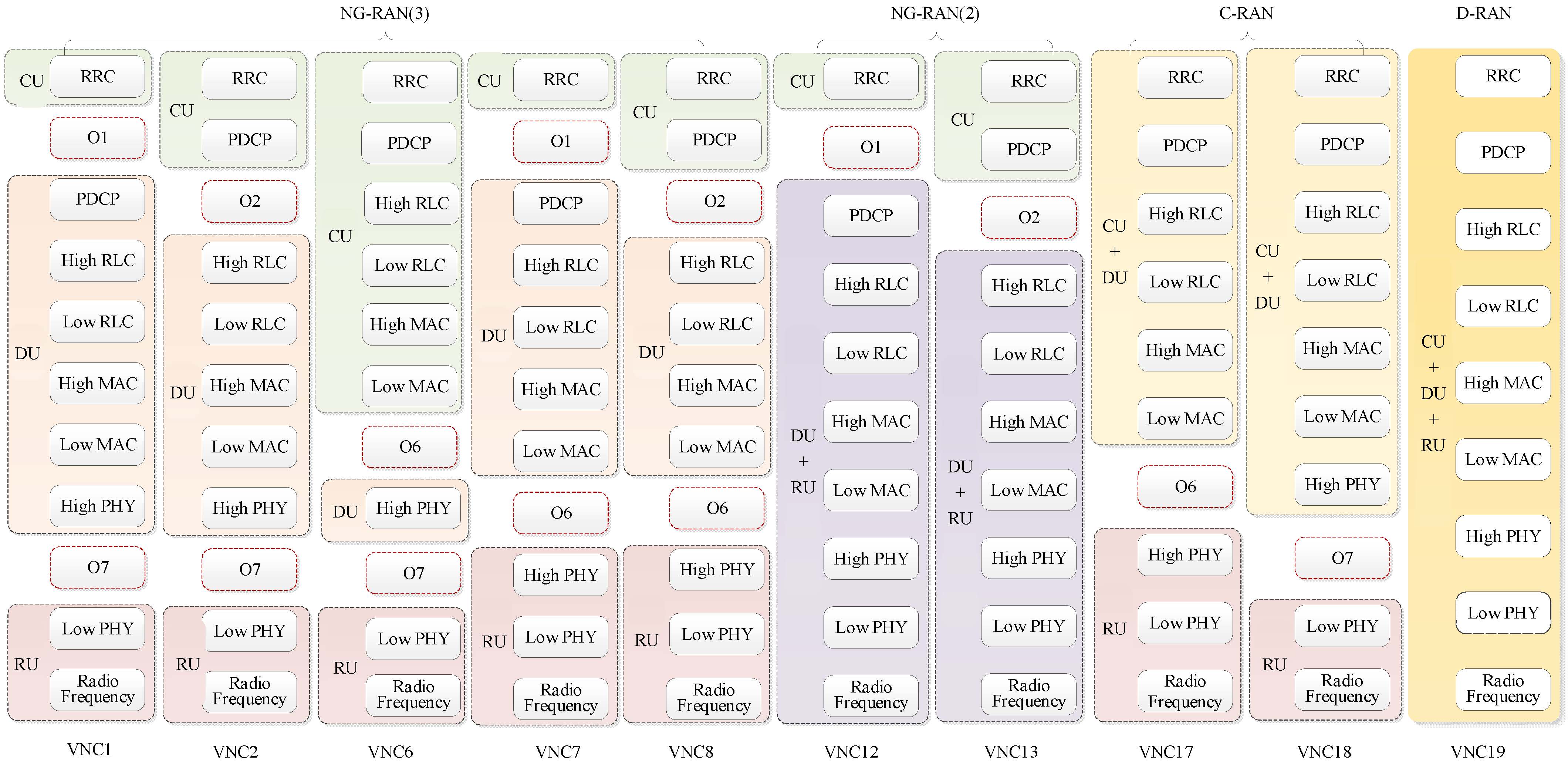
In this section, we define the system model and formally describe the problem of functional placement in vRAN. We first introduce the key elements of our system model, including the network architecture and resource constraints (Section 3.1). Then, we formulate the problem as an optimization challenge and define the objective function along with relevant constraints (Section 3.2).

Table 2. Model parameters and variables.

Notations	Descriptions
$G$	Topology of the vRAN
$V$	Set of nodes of $G$
$v_0$	Core network nodes
$B$	Set of BSs (RUs)
$T$	Set of transport nodes
$C$	Set of CNs
$e_{ij}^{Cap}$	Transmitting capacity of link $e_{ij}$
$e_{ij}^{Lat}$	Estimated latency $e_{ij}$
$v_i\in V$	Node of graph G
$N\left(v\right)$	Neighborhood of $v$
$P_i$	Set of the k-shortest routes for RU $b_i\in B$
$F$	Set of disaggregated RAN VNFs
$D$	Set of VNCs
$u_{ij}^m$	Indicates if $c_m\in C$ belongs to $p_{ij}\in P_i$
$M\left(c_m,f_s,b_i\right)$	Indicates if $c_m\in C$ runs $f_s\in F$ from $b_i\in B$
$z_{e_{ij}}^{P_{Bh}}$, $z_{e_{ij}}^{P_{Mh}}$, $z_{e_{ij}}^{P_{Fh}}$	Indicates if $e_{ij}$ is part of the backhaul, midhaul, and fronthaul
${\alpha }_{Bh}^r$, ${\alpha }_{Mh}^r$, ${\alpha }_{Fh}^r$	Bitrate demands in the backhaul, midhaul, and fronthaul for $D_r\in D$
${\beta }_{Bh}^r$, ${\beta }_{Mh}^r$, ${\beta }_{Fh}^r$	Maximum tolerated latency in the backhaul, midhaul, and fronthaul for $D_r\in D$
${\gamma }_m^s$	Computing demand of $f_s\in F$
$c_m^{Proc}$	Processing capacity of $c_m\in C$

summarizes the main notations used in this section.

3.1. System Model

In vRAN, the network function placement problem is a combinatorial optimization challenge. It requires making optimal joint decisions regarding the functional split of each BS function and the selection of routing paths. These decisions must satisfy constraints related to network transmitting performance and information processing capabilities, all while optimizing objectives such as minimizing costs. The functional split refers to disaggregating radio network functions (or protocol stacks) into various virtualized components that can be deployed different computing resources. The primary advantage of this approach is to enhance network performance and efficiency, allowing operators to tailor their networks to better meet user demands and optimize resource utilization. In the NG-RAN architecture, the functional split enables the separation of BS functions into three components: CU, DU, and RU [34]. There are eight potential functional options, each suited to different network requirements, such as latency, throughput, and deployment scenarios. Based on the concept of viable NG-RAN configurations (VNCs) established by standardization organizations and industry alliances [2,3], Figure 1 presents a set of VNCs considered, along with their respective functional split and the corresponding placement of VNF instances within their specific RAN nodes.

In Figure 1, O# represents a functional split option. Each split option imposes different communication requirements between vRAN nodes (CU, DU, and RU) in terms of minimum bitrate and maximum latency. The selection of a functional split depends on the characteristics of the underlying physical network and its ability to meet these requirements.

Table 3. 3GPP Latency and Bitrate Requirements for each split [2,3] (O7 split maximum value *).

Split Option	Functional Split	One-Way Maximum Latency	Minimum Bitrate (Gbps)
			Down Link	Up Link
O1	RRC–PDCP	10 ms	4	3
O2	PDCP–High RLC	10 ms	4	3
O3	High RLC–Low RLC	10 ms	4	3
O4	Low RLC–High MAC	1 ms	4	3
O5	High MAC–Low MAC	<1 ms	4	3
O6	Low MAC–High PHY	250 μs	4.13	5.64
O7	High PHY–Low PHY	250 μs	86.1 *	86.1 *
O8	Low PHY–Radio Frequency	250 μs	157.3	157.3

presents the latency and bitrate requirements associated with each functional split option. The values listed in Table 3 correspond to an RU with the following configuration: a 100 MHz bandwidth spectrum, 32 antenna ports, 8 MIMO layers, and 256 QAM modulation [2,3].

In a vRAN architecture, the CU and DU are virtualized nodes that can be deployed across various computing nodes, enabling resource sharing. Consequently, a single computing node can function as a virtual CU, a virtual DU, or both simultaneously. Moreover, CUs and DUs associated with different RUs can be placed on the same computing node, further enhancing resource efficiency. Therefore, by making informed decisions regarding functional splits and their placements, network operators can achieve optimized resource allocation and significantly enhance overall network performance.

We model a vRAN architecture with a graph $G=\{V,E\}$, where $V$ represents a collection of nodes, including a core network node $\left\{v_0\right\}$, a set $B=\{b_1,\dots ,b_{\left|B\right|}\}$ of RUs, a set $C=\{c_1,\dots ,c_{\left|C\right|}\}$ of computing nodes (CNs), and a set $T=\{t_1,\dots t_{\left|T\right|}\}$ of transport nodes, which may connect with RUs, CNs, the core node, or each other. $E=\{e_{ij};v_i,v_jϵV\}$ represents links, each characterized by a transmitting capability $e_{ij}^{Cap}$ and a latency $e_{ij}^{Lat}$ [23]. In this model, the Low PHY and Radio Frequency functions are typically placed in RUs, with the High PHY function also allocated to RUs in some VNCs [23]. The remaining functions are hosted in CUs or DUs, which are deployed on CNs. Each computing node $c_m\in C$ has a processing capability $c_m^{Pro}$ and other resources such as memory and storage, though these are not considered bottlenecks in our vRAN placement problem. Each RU is co-located with a CN. Transport nodes act as forwarding nodes only and do not perform vRAN functions. Typically, in cases where a transport node and a CN share the same location, the node is used as a computing node.

In this proposed vRAN graph model, the core node, $v_0$, serves as the source (downlink) or destination (uplink) of all network traffic. To maintain generality, we focus on the downlink scenario, but the model can easily be extended for the uplink. We define a set $P_i=\{p_{i1},\dots ,p_{ik}\}$ representing the $k$-shortest paths from the core node, $v_0$, to each RU $b_iϵB$. The data flow for each base station is unsplittable. Each path, $p_{ij}\in P_i$, contains at least sub-path $p_{Bh}$ (backhaul, i.e., core ↔ CU, core ↔ CU+DU, or core ↔ CU+DU+RU), and it may also include sub-paths $p_{Mh}$ (midhaul, i.e., CU ↔ DU, or CU ↔ DU+RU) and $p_{Fh}$ (fronthaul, i.e., RU ↔ DU, or RU ↔ CU+DU) [35]. Since Radio Frequency and Low PHY are always placed in the RU [14], we define a set $F=\{f_1,\dots {,f}_7\}$ to represent the remaining seven VNFs, where $f_7$ corresponds to RRC, $f_6$ to PDCP, and so on. The functional split must follow viable NG-RAN configurations (VNCs), identified by the set $D=\{D_1,\dots {,D}_{\left|D\right|}\}$ (as described in Figure 1). For each RU $b_i\in B$ in vRAN, the network function placement problem involves selecting an appropriate path $p_{ij}\in P_i$ and a VNC $D_r\in D$, and deploying $D_r$ on computing nodes along $p_{ij}$ while satisfying constraints on bandwidth, latency, and computational resources. The objective is to optimize overall radio access network performance. Figure 2 illustrates an example of function placement in vRAN. From Figure 2a, it can be seen that the CU is usually executed on more centralized and larger servers, while the DU is on relatively smaller servers, typically located near the RU. Figure 2b presents a topological graph model of the network shown in Figure 2a, constructed using our modeling formulas.

3.2. Function Placement Problem Formulation

In the function placement problem, we aim to make optimal joint decisions regarding both the selection of a routing path and its VNC for each RU $b_i\in B$. Our function placement problem formulation follows the approach described in [23], with modifications to adapt to the vRAN scenario. To represent these decisions, we define binary variables: $x_{ij}\in \left\{\mathrm{0,1}\right\}$ and $y_{ir}\in \left\{\mathrm{0,1}\right\}$, where $x_{ij}$ serve the RU $b_i\mathsf{ϵ}B$ through the path $p_{ij}\in P_i$, and $y_{ir}$ deploys the VNC $D_r\in D$ in the path $p_{ij}\in P_i$ for the RU $b_i\mathsf{ϵ}B$. This paper primarily focuses on two objectives: minimizing the number of active CNs used and maximizing the vRAN centralization level. In fact, a smaller number of active CNs leads to lower run costs for vRAN, while a higher centralization level results in greater network efficiency.

Formally, the objective function is defined as follows:

$$min \sum _{c_m\in C}{\Phi }_m-{\displaystyle \sum _{c_m\in C}}{\displaystyle \sum _{f_s\in F}}{\Psi }_{ms}$$

(1)

where ${\Phi }_m$ defines whether the CN $c_m\in C$ is used or not in the solution, its values are defined as follows:

$${\Phi }_m=\left\{\begin{array}{cc}1,\hfill & if {\displaystyle \sum _{b_i\in B}}{\displaystyle \sum _{p_{ij}\in P_i}}{{(x}_{ij}u}_{ij}^m)>0 for c_m\in C \hfill \\ 0,\hfill & otherwise \hfill \end{array}\right.$$

(2)

Moreover, ${\Psi }_{ms}$ determines the amount of $f_s\in F$ centralized in the CN $c_m\in C$ for different RUs, and its values are as follows:

$${\Psi }_{ms}=\left\{\begin{array}{c}{\displaystyle \sum _{b_i\in B}}M\left(c_m,f_s,b_i\right)-1, if {\displaystyle \sum _{b_i\in B}}{\displaystyle \sum _{p_{ij}\in P_i}}{{(x}_{ij}u}_{ij}^m)>0 for c_m\in C \\ 0, otherwise \end{array}\right.$$

(3)

In Equations (2) and (3), $u_{ij}^m\in \left\{\mathrm{0,1}\right\}$ indicates if the computing node $c_m\in C$ belongs to the path $p_{ij}\in P_i$, and the mapping function $M\left(c_m,f_s,b_i\right)\in \left\{\mathrm{0,1}\right\}$ indicates if the CN $c_m\in C$ runs the VNF $f_s\in F$ to serve the RU $b_i\in B$. Moreover, Equation (3) implies that if a CN $c_m\in C$ is utilized, more RUs are required to deploy their VNF $f_s\in F$ on $c_m$ to achieve a higher centralization level. In this type of problems, the following constraints must be satisfied when making decisions.

A. 

Combinational constraints

For each RU $b_i\in B$, only one path $p_{ij}\in P_i$ and one VNC $D_r\in D$ are selected to satisfy its service requirements. The constraints represented are defined as follows:

$${\sum }_{j=1}^k{x}_{ij}=1, {\forall b}_i\in B$$

(4)

$${\sum }_{r=1}^{\left|D\right|}{y}_{ir}=1, {\forall b}_i\in B$$

(5)

B. 

Link capacity constraints

To prevent the solution from exceeding link capacities, for each link $e_{ab}\in E$, the total demand on link $e_{ab}$, driven by all fronthaul (${\alpha }_{Fh}^r$), midhaul (${\alpha }_{Mh}^r$), and backhaul (${\alpha }_{Bh}^r$) must not surpass the transmission capacity $e_{ab}^{Cap}$. This is represented by the following constraint:

$$\sum _{D_r\in D}\sum _{b_iϵ\mathrm{B}}\sum _{p_{ij}\in P_i}{x}_{ij}{y}_{ir}\left(z_{e_{ab}}^{P_{Fh}}{\alpha }_{Fh}^r+z_{e_{ab}}^{P_{Mh}}{\alpha }_{Mh}^r+z_{e_{ab}}^{P_{Bh}}{\alpha }_{Bh}^r\right)\le e_{ab}^{Cap}, \forall e_{ab}\in E$$

(6)

where $z_{e_{ab}}^{P_{Fh}}$, $z_{e_{ab}}^{P_{Mh}}$, and $z_{e_{ab}}^{P_{Bh}}\in \{0,1\}$ represents whether the link $e_{ab}$ is part of fronthaul, midhaul, and backhaul, respectively. If so, the value will be equal to the unit; otherwise, it is 0. Moreover, ${\alpha }_{Fh}^r$, ${\alpha }_{Mh}^r$, and ${\alpha }_{Bh}^r$ denote a bitrate demand of VNC $D_r$ in the fronthaul, midhaul, and backhaul, respectively.

C. 

Tolerable latency constraints

For each RU $b_i\in B$, a specific VNC $D_r\in D$ is deployed along the selected path $p_{ij}\in P_i$. The latency of each sub-path-backhaul, midhaul, and fronthaul-within $p_{ij}$ must not exceed the corresponding maximum tolerable latency of the VNC $D_r$. Thus, here are the following constraints:

$$\sum _{e_{ab}\in E}{x}_{ij}{y}_{ir}{z}_{e_{ab}}^{P_{Bh}}{e}_{ab}^{Lat}\le {\beta }_{Bh}^r,\hspace{1em}\hspace{1em}\forall b_i\in B,p_{ij}\in P_i,D_r\in D$$

(7)

$$\sum _{e_{ab}\in E}{x}_{ij}{y}_{ir}{z}_{e_{ab}}^{P_{Mh}}{e}_{ab}^{Lat}\le {\beta }_{Mh}^r,\hspace{1em}\hspace{1em}\forall b_i\in B,p_{ij}\in P_i,D_r\in D$$

(8)

$$\sum _{e_{ab}\in E}{x}_{ij}{y}_{ir}{z}_{e_{ab}}^{P_{Fh}}{e}_{ab}^{Lat}\le {\beta }_{Fh}^r,\hspace{1em}\hspace{1em}\forall b_i\in B,p_{ij}\in P_i,D_r\in D$$

(9)

where ${\beta }_{Bh}^r$, ${\beta }_{Mh}^r$, and ${\beta }_{Fh}^r$ denote the maximum tolerated latency in backhaul, midhaul, and fronthaul for $D_r\in D$, respectively.

D. 

Processing capacity constraint

For each CN $c_m\in C$, all VNFs deployed in $c_m$ must be smaller than its processing capacity $c_m^{Proc}$. Thus, the processing capacity constraint is defined by the following:

$$\sum _{f_s\in F}\sum _{b_iϵ\mathrm{B}}\sum _{p_{ij}\in P_i}\sum _{D_r\in D}{x}_{ij}{y}_{ir}{u}_{ij}^{m}M\left(c_m,f_s,b_i\right){\gamma }_m^s\le c_m^{Proc},\hspace{1em}\hspace{1em}\forall c_m\in C$$

(10)

where ${\gamma }_m^s$ represents the computing demand of the VNF $f_s\in F$.

From the previous description, the vRAN function placement problem can be formulated as a mixed integer nonlinear model. It has been proven to be NP-hard through a polynomial reduction in the multiple-choice multidimensional knapsack problem [24]. Therefore, the solution space grows exponentially with increasing network scale, making it increasingly difficult for traditional methods to find optimal solutions. Therefore, we employ a DRL approach to address this complex problem.

4. DRL Method Based on GNN for Function Placement Problems

In this section, we present a DRL method based on GNN, referred to as GDRL, for solving the function placement problems. Figure 3 illustrates the overall framework of this approach. In this method, the agent consists of an actor and a critic, both modeled using a GNN that incorporates node and link features. By embedding nodes and edges into a latent feature space, the GNN enables the agent to obtain a more accurate representation of the current state [36]. Therefore, the actor can generate a more accurate action selection policy, while the critic provides a more reliable evaluation off the policy. The detailed training process for this DRL framework is described in Section 4.2.3. The following subsections provide an in-depth explanation of this method.

4.1. Three Essential Elements of DRL

State, action, and reward are the three essential elements of an RL framework [37]. In the following, we will describe them for the function placement problem.

4.1.1. State Representation

To effectively generate function placement policies using GDRL, the state representation must not only accurately describe the environment but also reflect the complex topology of the RAN. In our model, to learn node embeddings and edge embeddings, we construct a line graph $G_e$ from the given graph $G$. The construction method is as follows: each edge $(v_i,v_j)$ in the original graph $G$ corresponds to a vertex $v_{ij}$ in the line graph $G_e$. Furthermore, if edges $(v_i,v_j)$ and $(v_j,v_k)$ in $G$ share a common vertex $v_j$, then in the line graph $G_e$, there is an edge $\left(v_{ij},v_{jk}\right)$. The state representation mainly includes the network structure, node features, and link features. We use adjacency matrixes $A_v$ and $A_e$ corresponding to the topology of graph $G$ and its line graph $G_e$, respectively. Each node feature in graph $G$ is represented by a feature vector, which mainly includes the following: (1) node type, where a value of 1 is assigned if it is an RU node, and 0 otherwise; (2) remaining computational capacity, which represents the remaining computational capacity value if it is an CN, otherwise 0; (3) remaining demand, representing the remaining demand value if it is an RU node, otherwise 0. Similarly, every edge feature in $G$ is represented by a feature vector, which mainly includes features such as the remaining transmitting capability and the maximum delay [38]. A node feature in line graph $G_e$ corresponds to an edge feature in original graph $G$. For a graph with $N_v$ nodes and $N_e$ edges, the node features and edge features can be represented as a matrix $X_v$ of size $N_v\times F_v$ for node features and a matrix $X_e$ of size $N_e\times F_e$ for edge features, where $F_v$ and $F_e$ denote the dimensions of the node and edge feature vectors, respectively.

4.1.2. Action Space

In our model, we need to select an appropriate path and its corresponding VNC for each RU. To achieve this, we define the action space as a set of tuples $(p_t,d_t)$, representing the allocation configurations for the RUs, where pt and dt correspond to the binary decision variables $x_{ij}$ and $y_{ir}$, which determine the path selection and VNC deployment for a RU $b_i$, respectively. However, considering every possible path would cause the action space to grow exponentially as the network scales up. This results in a higher computational burden and slower convergence during optimization. To mitigate this issue, we define a candidate path set $P_i=\{p_{i1},\dots ,p_{ik}\}$ for each RU $b_i\mathsf{ϵ}B$, using the $k$-shortest path algorithm from the core node $v_0$ to $b_i$. Figure 1 lists the VNCs (except VNC6) considered in the proposed model. Thus, the size of the action space $A$ is represented as follows:

$$|A|=\left|D\right|\sum _{b_i\in B}\left(\left|P_i\right|\right)$$

(11)

4.1.3. Reward Design

The principle of reward design is that a smaller number of CNs and a higher centralization level result in a higher reward. An action is considered valid if the selected path and its VNC satisfy all the constraints described in Equations (4)–(10), in which case a positive reward is assigned. Otherwise, the action receives a negative reward as a penalty. For a valid action $a_t=(p_t,d_t)$, the reward is computed based on the newly added number $\nabla {\Phi }_t$ of computation nodes and the newly increased concentration degree ${\nabla \Psi }_t$ after adopting this action utilizing the objective function Equation (1). For an invalid action $a_t=(p_t,d_t)$, the reward is determined by calculating the number $\left|B_{t-1}\right|$ of Rus, which have already been allocated resources in the previous step. Thus, the reward $r\left(a_t\right)$ is expressed as follows:

$$r\left(a_t\right)=\left\{\begin{array}{c}{\nabla \Psi }_t-\nabla {\Phi }_t , if \left(pt,dt\right) is valid. \\ \left|B_{t-1}\right|-\left|B\right|, otherwise \end{array}\right.$$

(12)

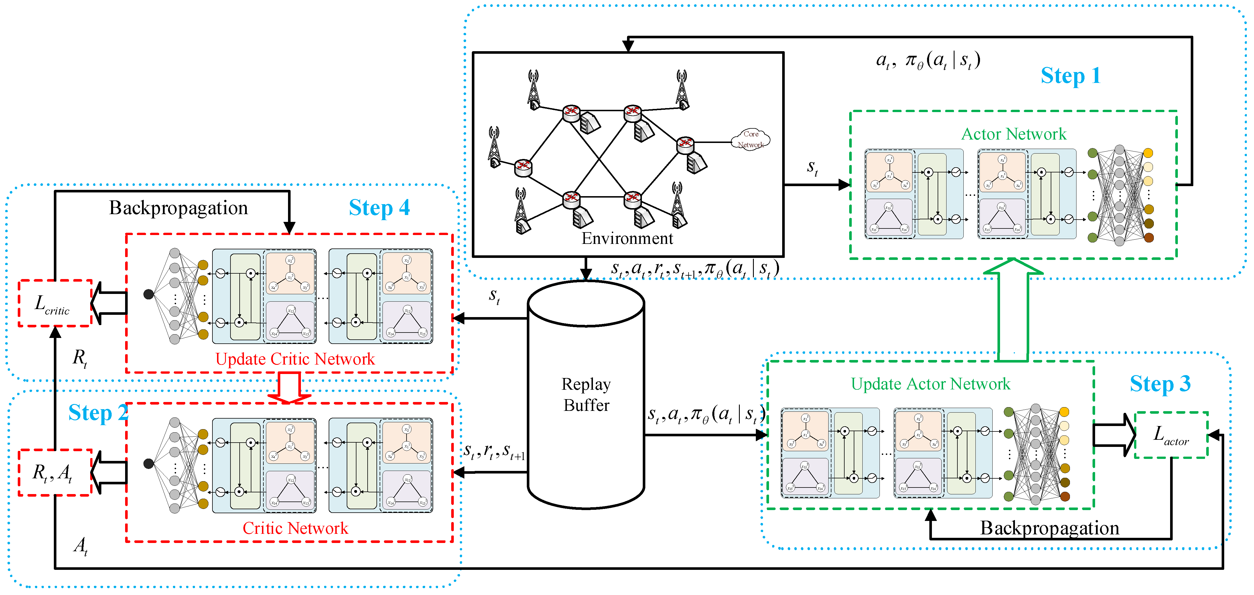
4.2. Graph Proximal Policy Optimization

Proximal Policy Optimization (PPO) [39] was introduced in 2017 as a policy gradient method for training the DRL model. Since then, it has been widely adopted across various DRL tasks, including robotics, autonomous vehicles, and natural language processing. PPO is an actor-critic type algorithm, where both the actor and critic networks are typically implemented using Multi-Layer Perceptron (MLP) [40]. In recent years, researchers have integrated GNNs into actor-critic architectures to enhance DRL’s capability to process graph-structured data, leading to significant performance improvements [41,42,43]. However, most GNNs primarily apply convolution operations on node features, often overlooking the valuable information present in edge features [44]. Consequently, these models are less suitable for solving network function placement problems where both node and edge features play a critical role in decision-making. Recently, Jiang et al. proposed a GNN-based model called CensNet, which effectively embeds both node and edge features into a latent feature space [36]. This innovative framework enables CensNet to address function placement challenges that depend on both types of features [45]. In this subsection, we explore the GPPO algorithm, which integrates CensNet to effectively solve the function placement problem. Below, we provide a detailed description of each component.

4.2.1. Actor Network

In the function placement problem, it is crucial not only to deploy functions based on RUs demands and the processing capabilities of the computing nodes, but also to meet the constraints of link bandwidth and latency. Therefore, the agent must have comprehensive information about both node and edge features to make precise and effective decisions. Our actor network consists of three-layer GNN combined with a two-layer fully connected network, as shown in Figure 4. The GNN is responsible for accurately extracting the features of both nodes and links, while the fully connected network focuses on learning decision-making patterns to generate appropriate actions. The GNN uses CensNet [36], which stands apart from traditional GNNs that only learn node embeddings. CensNet alternately between learning and updating node and edge embeddings, effectively embedding both node and edge features into a shared latent feature space [44]. Below, we provide a detailed description of the propagation rules within CensNet.

Given a graph $G_v$ with $N_v$ nodes and $N_e$ edges, let $A_v$, $X_v$, and $X_e$ represent the adjacency matrix, node feature matrix, and edge feature matrix of $G_v$, respectively. Let $G_e$ be the line graph of $G_v$ and $A_e$ be the adjacency matrix of $G_e$. Let $H_v^{\left(l\right)}$ and $H_e^{\left(l\right)}$ represent the output of the node features and edge features at the l-layer, respectively. The initial features are given $H_v^{\left(0\right)}=X_v$ and $H_e^{\left(0\right)}=X_e$, and $I_{N_v}$ and $I_{N_e}$ represent the identity matrices. $D_v$ and $D_e$ are the diagonal degree matrices of $A_v+I_{N_v}$ and $A_e+I_{N_e}$, respectively. As shown in Figure 4, our actor architecture integrates a three-layer GNN for feature extraction, which is then connected to a two-layer fully connected module. Each layer of the GNN incorporates both a graph convolution operation and a fusion operation. In the graph convolution operation, an approximated spectral graph convolution is used. The normalized Laplacian adjacency matrices of graphs $G_v$ and $G_e$ are defined in Equations (13) and (14), respectively.

$${\tilde{A}}_v=D_v^{-{\displaystyle \frac{1}{2}}}(A_v+I_{N_v})D_v^{-{\displaystyle \frac{1}{2}}}$$

(13)

$${\tilde{A}}_e=D_e^{-{\displaystyle \frac{1}{2}}}(A_e+I_{N_e})D_e^{-{\displaystyle \frac{1}{2}}}$$

(14)

The layer-wise propagation rule for node features in the ($l+1$)-th layer is defined as follows:

$$H_v^{(l+1)}=\sigma \left(T\mathsf{\Phi }\right(H_e^{\left(l\right)}{P}_e)T^T⨀{\tilde{A}}_v{H}_v^{\left(l\right)}{W}_v)$$

(15)

where $\sigma (.)$ is an activation function, the matrix $T$ is the incidence matrix of graph $G_v$, and $T_{im}$ represents whether the edge $m$ connects node $i$. Moreover, $P_e$ is a $F_e$-dimensional vector, defined as the learnable weights for edge feature vectors. In addition, $\mathsf{\Phi }(.)$ denotes the diagonalization operation of a square matrix, whereas $⨀$ denotes the Hadamard product or element-wise product, and $W_v$ is a learnable weight matrix, updated in the training stage of reinforcement learning [36].

Referring to Figure 4, the graph convolution operation in $G_v$ corresponds to the term ${\tilde{A}}_v{H}_v^{\left(l\right)}{W}_v$ of Equation (15). This propagation rule in Equation (5) can be understood as mapping corresponding elements from $T\mathsf{\Phi }\left(H_e^{\left(l\right)}{P}_e\right)T^T$ to the normalized node adjacency matrix. Moreover, $T\mathsf{\Phi }\left(H_e^{\left(l\right)}{P}_e\right)T^T⨀{\tilde{A}}_v$ represents a fused node adjacency matrix, generated by integrating information from the counterpart of the line graph $G_e$. Therefore, the term $T\mathsf{\Phi }\left(\right(.{)P}_e)T^T⨀(.)$ of Equation (15) is defined as the fusion operation integrating the edge embedding into node embedding.

Similarly, the layer-wise propagation rule for edge features is expressed as follows:

$$H_e^{(l+1)}=\sigma \left(T^T\mathsf{\Phi }\right(H_v^{\left(l\right)}{P}_v)T⨀{\tilde{A}}_e{H}_e^{\left(l\right)}{W}_e)$$

(16)

where $P_v$ represents the learnable weights for node feature vectors. Moreover, $W_e$ is a learnable weight matrix updated in the training stage of the reinforcement learning. Similarly, the graph convolution operation in graph $G_e$ corresponds to the term ${\tilde{A}}_e{H}_e^{\left(l\right)}{W}_e$ of Equation (16) and the fusion operation corresponds to the term $T^T\mathsf{\Phi }\left(\right(.\left)P_v\right)T⨀(.)$.

Since the features of nodes and edges extracted using GNNs are multidimensional, they must be flattened to one vector and further exploited by fully connect layers.

As illustrated in Figure 4, the processing pipeline of the actor network proceeds as follows. Initially, the adjacency matrix $A_v$ and the corresponding node feature matrix $X_v$ are extracted from the underlying topological environment. Subsequently, a line graph is constructed to obtain the adjacency matrix $A_e$ and node feature matrix $X_e$. These inputs are then fed into a three-layer Graph Neural Network (GNN). Within each GNN layer, graph convolution and feature fusion operations are performed to capture expressive representations of both nodes and edges. The resulting features are subsequently flattened and passed through a two-layer fully connected network. This processing ultimately yields the action selection policy.

4.2.2. Critic Network

The critic network in the proposed architecture mirrors the actor network, as illustrated in Figure 5. It consists of three layers of GNN followed by two fully connected neural networks layers. It leverages the GNN to extract features from nodes and edges, which are subsequently linearly mapped to a scalar value through the fully connected layers. This scalar value is further used in both parameter updates and action evaluations.

4.2.3. GPPO Algorithm

The PPO algorithm is a well-known policy gradient method in DRL due to its effective balance between exploration and exploitation, alongside stable learning ability. In the DRL model, the GPPO algorithm runs for $N$ epochs, where in each epoch, the agent interacts with the environment for $T$ steps, and both the actor and critic networks update their parameters $M$ times. To describe the training process, the following notations and functions are used. In the $i$-th epoch, the actor network is denoted as ${\pi }_{{\theta }_i}$ and the critic network as $V_{{\varphi }_i}$, where ${\theta }_i$ and ${\varphi }_i$ are the parameters of the actor and critic networks, respectively. These parameters include the weights of the GNNs ($W_v$, $W_e$, $P_v$, and $P_e$), as well as the parameters of the fully connected layers. At each interaction, $s_t$, $a_t$, and $r_t$ represent the state, action, and reward, respectively, where ${\pi }_{{\theta }_i}\left(a_t\right|s_t)$ represents the probability of the actor network ${\pi }_{{\theta }_i}$ selection action $a_t$ at state $s_t$.

With the above notations, the advantage $A_t\left({\theta }_i\right)$ of the action ${\theta }_i$ in state $s_t$ is computed using the following formula.

$$A_t\left({\theta }_i\right)=R_t-V_{{\varphi }_i}\left(s_t\right)$$

(17)

where $V_{{\varphi }_i}\left(s_t\right)$ represents the current value function from the critic network. The return $R_t$ can be computed as follows:

$$R_t=r_t+\gamma V_{{\varphi }_i}\left(s_{t+1}\right)$$

(18)

where $\gamma$ is the discount factor.

The loss function of the actor network in the updating process is defined as follows:

$$L_{actor}\left(\theta \right)=E\left[\min \left\{{\rho }_t\left(\theta \right)A_t\left({\theta }_i\right),clip({\rho }_t\left(\theta \right),1-ϵ,1+ϵ,A_t\left({\theta }_i\right))\right\}\right]$$

(19)

where $E[.]$ indicates the empirical average over a finite batch of samples in the replay buffer, $ϵ$ is a hyperparameter to decide the size of clipping, and ${\rho }_t\left(\theta \right)$ denotes the probability ratio of the policy value before and after the update of the actor network; it is expressed as follows:

$${\rho }_t\left(\theta \right)={\displaystyle \frac{{\pi }_{\theta }\left(a_t\right|s_t)}{{\pi }_{{\theta }_i}\left(a_t\right|s_t)}}$$

(20)

Moreover, the clipping function $clip(.,.,.,.)$ is defined as follows:

$$clip\left(a,b,c,d\right)=\left\{\begin{array}{c}\min \left\{a,c\right\}·d, if d>0 \\ \min \left\{a,b\right\}·d otherwise\hfill \end{array}\right.$$

(21)

In Equation (18), ${\rho }_t\left(\theta \right)A_t\left({\theta }_i\right)$ represent the common objective of the actor-critic framework, while $clip({\rho }_t\left(\theta \right),1-ϵ,1+ϵ,A_t\left({\theta }_i\right))$ modifies this objective by clipping the probability ratio ${\rho }_t\left(\theta \right)$. This modification helps to achieve the stability of the training process.

On the other hand, the loss function for updating the critic network is defined as follows:

$$L_{critic}\left(\varphi \right)=E\left[A_t^2\left({\theta }_i\right)\right]$$

(22)

Figure 3 and Algorithm 1 fully describe the iterative processes of the PPO algorithm. The following four main stages of every epoch of the training processing are determined in Algorithm 1.

Algorithm 1. GPPO Algorithm
	Input: $e_{ij}^{Cap}$,$e_{ij}^{Lat}$, $c_m^{Proc}$, discount, learning rate, Clipping parameter
	Output: final actor parameters ${\theta }_N$, final critic parameters ${\varphi }_N$
1:	Initialize: the parameter ${\theta }_0$ of the actor network ${\pi }_{{\theta }_i}$;
	the parameter ${\varphi }_0$ of the critic network $V_{{\varphi }_i}$;
	iteration epochs $N$, updating times $M$ of every epoch.
2:	for $i=\mathrm{1,2},\dots ,N$ do
3:	Empty replay buffer B and reset the environment;
4:	$s_t=s_0$;
5:	for $t=\mathrm{1,2},\dots ,T$ do
6:	Sample action $a_t$ based on ${\pi }_{{\theta }_i}\left(a_t\right|s_t)$;
7:	Execute action $a_t$ and obtain next state $s_{t+1}$;
8:	Compute reward $r_t$ according to Equation (12);
9:	Store experience $(s_t,{a_t,r}_t,s_{t+1},{\pi }_{{\theta }_i}(a_t\left|s_t\right))$ in replay buffer B;
10:	Compute the return $R_t$ according to Equation (17);
11:	Estimate the advantage $A_t\left({\theta }_i\right)$ from $V_{{\varphi }_i}\left(s_t\right)$ according to Equation (18);
12:	end for
13:	for $j=\mathrm{1,2},\dots ,M$ do
14:	Sample a batch of experiences $D$ from replay buffer B;
15:	${\theta }_{i,j}\leftarrow \arg \max L_{actor}\left(\theta \right)$ according to Equation (19);
16:	${\varphi }_{i,j}\leftarrow \arg \min L_{critic}\left(\varphi \right)$ according to Equation (22);
17:	end for
18:	${\theta }_{i+1}\leftarrow {\theta }_{i,j}$, and ${\varphi }_{i+1}\leftarrow {\varphi }_{i,j}$;
19:	end for

The implementation of the GPPO algorithm involves four essential phases, which we detail below for better comprehension of its interaction with the environment and the update process.

(1)

Interaction with the environment (lines 6–9): the actor network interacts with the environment of the network functional placement problem, then samples an action $a_t$ from the action distribution given state $s_t$, executes the action $a_t$ in the environment and receives a reward at the next state $s_{t+1}$, and stores the experience in the buffer. The above operations are repeated to collect training data. These data are generated through interaction with a simulated vRAN environment.

(2)

Compute advantages (lines 10–11): compute the value function $V_{{\varphi }_i}\left(s_t\right)$ for every state $s_t$ using the critic network and compute the return $R_t$ and the advantage $A_t\left({\theta }_i\right)$ based on the current critic network.

(3)

Update the actor network (line 15): based on the sample data in the reply buffer and the advantage $A_t\left({\theta }_i\right)$, the actor network is updated by maximizing the PPO-Clip objective.

(4)

Update the critic network (line 16): similarly, the critic network is updated using the Mean Squared Error (MSE) between the estimated values and the computed returns.

5. Performance Evaluation

In this section, we conduct simulation experiments on RAN scenarios for seven different scales and assess the effectiveness of our presented GDRL method by comparing it to three related methods. All experiments run on a computer with 6-core Intel(R) i5-10400F 2.9 GHz CPU, 16 GB RAM, and NVIDIA GeForce RTX 3060TI 8 GB GPU. We use PyTorch to implement the GDRL method in the Pycharm develop platform and Adam to optimize the actor and critic networks.

5.1. Baseline Methods and Simulation Setup

To evaluate the performance of the GDRL method, we compare it to the DRL method [23] and PlaceRAN [12], since they all address a similar system model. Moreover, the proposed GDRL method is inspired by the DRL method [23] to solve the placement problem. In addition, the GDRL method is compared to the optimal method proposed by Murti [10] to check its performance when considering simplified system model, which only considers a fixed CU, a set of fixed DUs, and only one path for each RU. Therefore, our evaluation is conducted based on two distinct scenarios:

(1)

The first case does not consider routing, where a single path is assigned for functional split for each RU, corresponding to the system model proposed by Mutri [10];

(2)

The second case considers routing, where functional split and function placement must be decided from multiple paths for each RU, reflecting the system model proposed in this paper. Therefore,

Table 4. Parameters employed.

Parameters	Values
|$B$|	{5, 10, 19, 35, 80, 122, 213}
|$C$|	{8, 16, 32, 64, 128, 256, 512}
|$D$|	{4, 9}
$e_{ij}^{Cap}$(Gpbs)	{200, 400, 800, 1000}
$e_{ij}^{Lat}$(ms)	{0.163, 0.22, 0.29}
$c_m^{Proc}$(cores)	{8, 16, 32, 64}
epochs	5000
Timestep	5000
Batch size	50
discount	0.99
learning rate	0.001
Clipping parameter	0.3

presents the parameters and information about the network resources employed in these experiments.

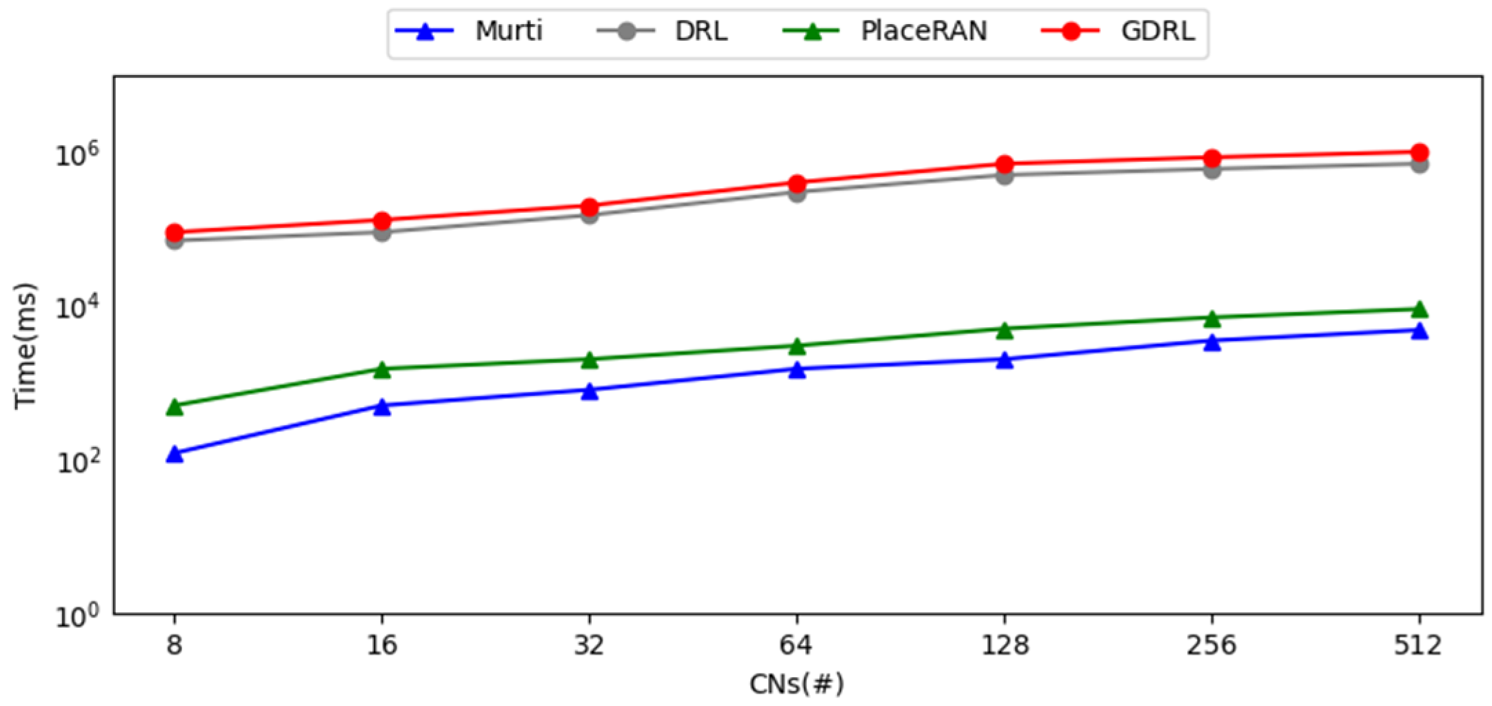
5.2. Evaluation Without Routing Decisions

To compare the performance of the proposed method with Murti [10], PlaceRAN [12], and DRL [23], we considered RANs with 8, 16, 32, 64, 128, 256, and 512 nodes. When neglecting routing, all instances used the limitations of the model presented by Murti [10]. Murti’s model considered only VNCs 2, 6, 18, and 19, while the other methods use nine VNCs as shown in Figure 1 (except VNC 6). Figure 6 illustrates the centralization level of VNFs for each model while neglecting considering routing. As depicted in Figure 6, in small-scale scenarios, such as those handling up to 32 nodes, the Murti and PlaceRAN methods achieve the same centralization level, while DRL and GDRL approaches are roughly comparable, albeit slightly lower than those attained by the first two methods. As the number of CNs and RUs increases, the centralization level achieved by the Murti method is consistently lower than that of the other approaches. Notably, in scenarios involving 256 and 512 CNs, the Murti method exhibits a downward trend in centralization level. This can be attributed to the fact that this method considers only four forms of VNCs for functional split. In smaller scales, the limited number of RUs results in minimal impact on the algorithm’s ability to place functions effectively. However, as the scale increases, these four forms of functional split restrict the algorithm’s function placement capabilities. In contrast, by considering nine forms of VNCs for functional split and more vRAN nodes, the other three methods can identify more effective solutions. For instance, the PlaceRAN method can find the optimal solution for each instance. Consequently, it demonstrates the best centralization level among the evaluated methods. Referring to Figure 6, the GDRL method exhibits a higher centralization level compared to the DRL method, which also shows instability, specifically at 256 CNs. This discrepancy can be explained by the fact that the GDRL method uses the GPPO policy gradient algorithm, employing GNNs to extract feature information from both nodes and edges. This capability allows the agent to acquire more comprehensive information for policy learning and evaluation, resulting in more accurate decision-making. In opposite, the DRL method predominantly relies on node information during policy learning and evaluation, often overlooking edge feature information, which detrimentally affects the agent’s ability to make effective decisions.

Figure 7 illustrates the execution times of these methods across network scenarios for varying CN numbers. In more detail, the Murti method exhibits the shortest execution time due to its relatively simple model, considering only four forms of function splitting. In contrast, the PlaceRAN method considers nine forms of function splitting but does not incorporate routing; therefore, it performs function placement along a single path. Consequently, it can reach the optimal solution for the problem under these constraints, leading to faster execution time and demonstrating robust performance. However, the execution times for the DRL and GDRL methods are slower than those of PlaceRAN and Murti, as they consider the training time. Notably, the execution time grows exponentially, the execution time of DRL is shorter than that of GDRL. This discrepancy arises from the inclusion of the GNN module in the GDRL approach, which increases the training time. However, the GDRL agent can make better efficient decisions, leading to a reduction in the number of iterations to some extent. Nonetheless, the overall execution time remains slightly higher than that of DRL.

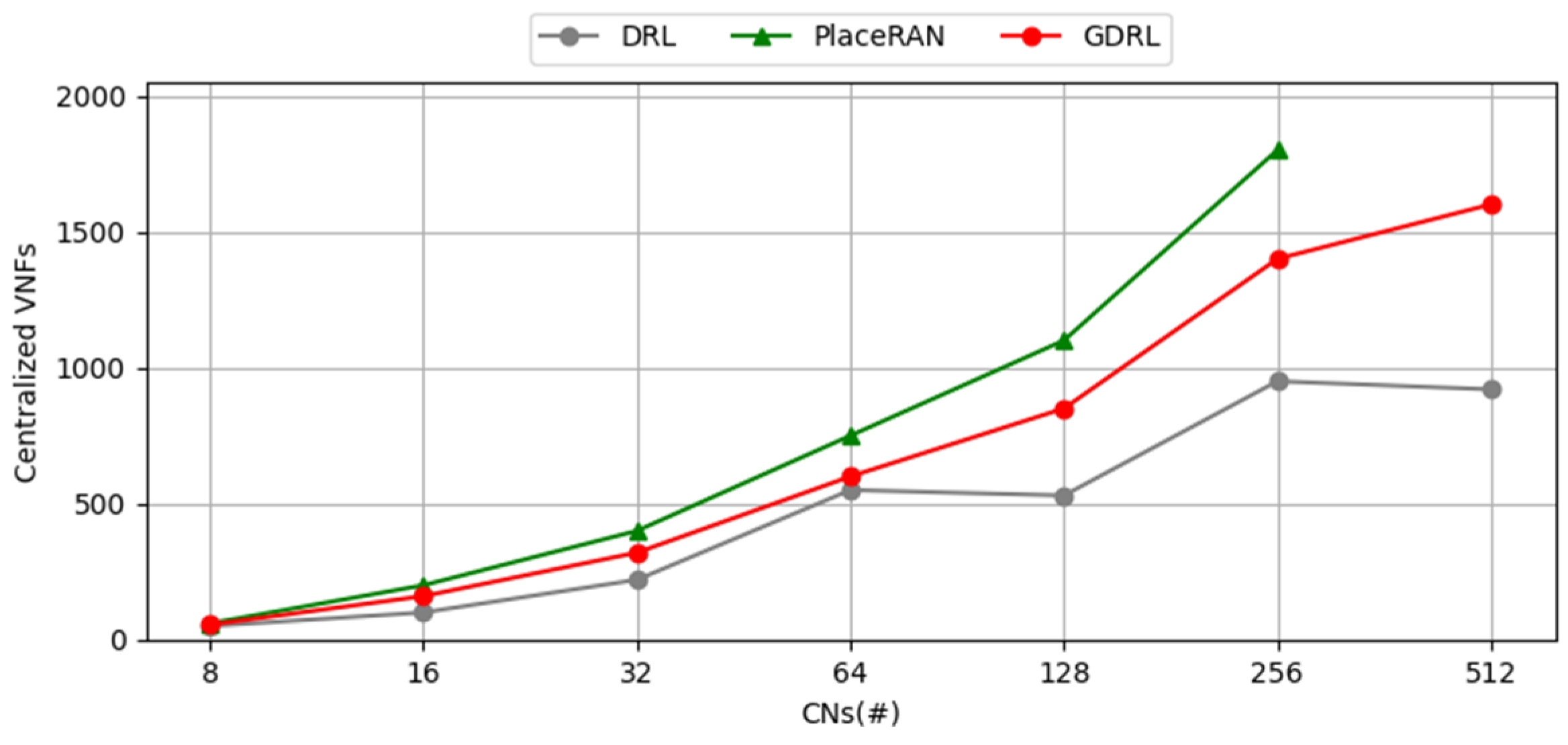
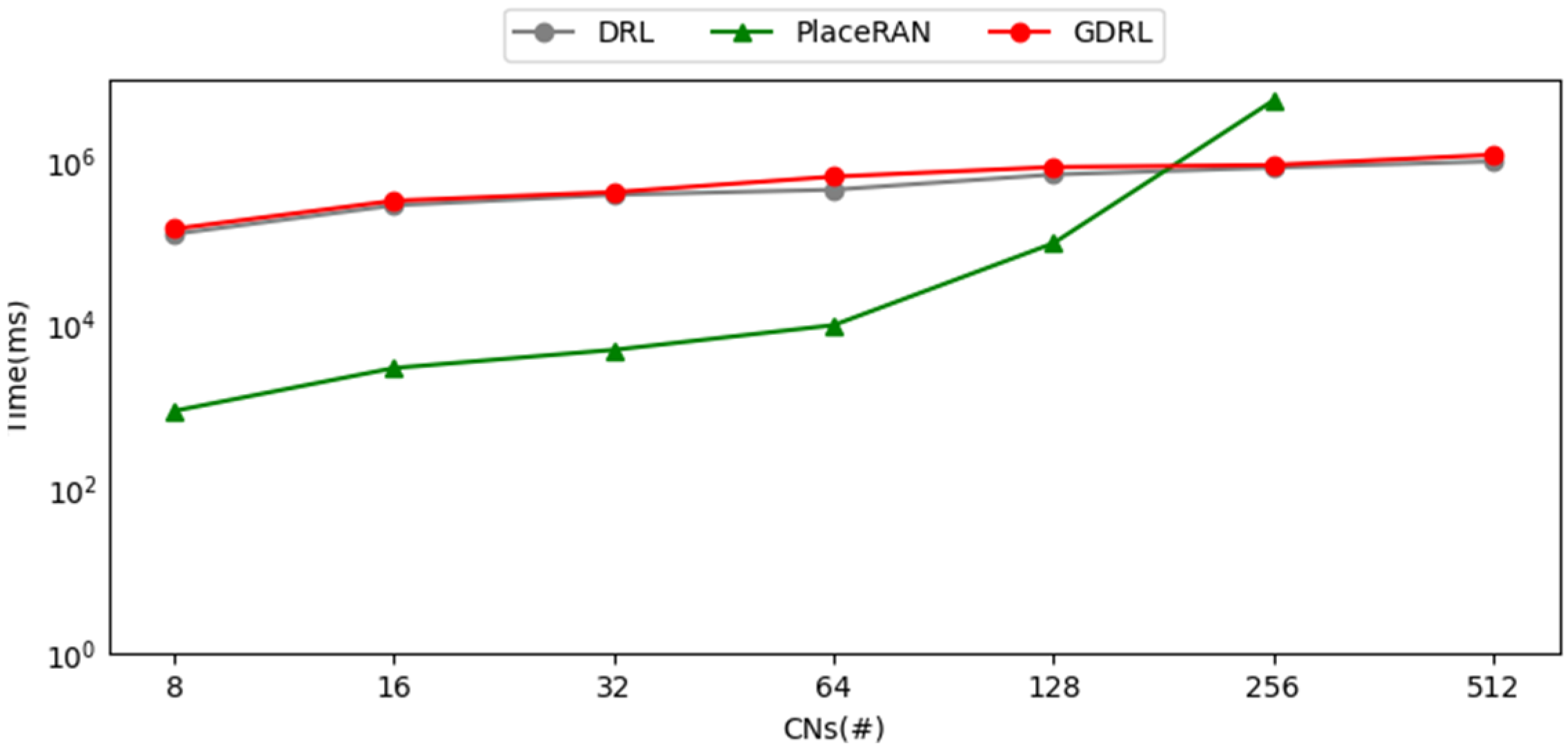
5.3. Evaluation with Routing Decisions

The same evaluation methodology is applied as described in the previous subsection to compare the performance of the placement, DRL, and GDRL methods. In the proposed experiments, we investigate the placement problem for each RU while considering nine different forms of function splitting and four possible distinct routings. Figure 8 and Figure 9 illustrate the centralization level of VNFs and execution time for each model while considering routing, respectively. By comparing Figure 6 and Figure 8, we observe that, when routing is considered, all models can identify superior solutions and achieve higher centralization levels. Consequently, incorporating routing considerations into decision-making is beneficial for the allocation and management of network resources. Moreover, from Figure 8 and Figure 9, it is evident that the PlaceRAN method achieves the highest level of centralization. However, as the size of the instances increases, the time required for execution significantly increases. When dealing with 256 CNs, the computing time of PlaceRAN surpasses that of DRL and GDRL. Notably, it becomes inoperable when the number of CNs reaches or exceeds 512. In contrast, both DRL and GDRL can solve the functional placement problem for all instances. However, it is clear that the centralization level of the DRL method decreases at 128 and 512 nodes, indicating that its performance lacks stability. On the other hand, the GDRL method, which utilizes the GPPO gradient strategy, demonstrates more consistent performance. For each instance, the centralization level achieved by this method surpasses that of DRL. Although the execution time of GDRL is slightly greater than that of DRL, it outperforms DRL.

6. Discussion

Our findings demonstrate that the proposed method performs well in both small-scale and large-scale vRANs. Although it shows slightly reduced centralization level compared to optimal approaches in small-scale vRANs, our method remains fully operational in large-scale routing-aware networks. One limitation of this study is the lack of consideration for dynamic network conditions, which may affect the generalizability of the results. Future work should focus on adapting the model to real-time dynamic environments.

7. Conclusions

In this work, we formulate the network function placement problem in vRAN as a mixed-integer nonlinear programming model. To address this model, we proposed a Deep Reinforcement Learning approach (GDRL) based on Graph Neural Networks (GNNs). The GPPO gradient policy algorithm was introduced to ensure policy stability during the reinforcement learning training process. The GNNs were incorporated into both the actor and critic networks to effectively capture node and edge features, ensuring the agent has more accurate and comprehensive observational data, which leads to better decision-making, faster training, and enhanced overall algorithm performance. Comparative evaluations against other approaches indicate that our GDRL method achieves superior performance, particularly in terms of network centralization and the ability to handle large-scale RAN scenarios. Key contributions of this work include the development of a mixed-integer nonlinear programming model to integrate the functional split and network function placement problems. Our model optimizes the allocation of computing resources with the goal of minimizing resource usage and maximizing the centralization level of the vRAN. And we proposed an efficient DRL algorithm using the GPPO framework. We integrated GNNs that combine both node and edge embeddings into the actor and critic networks, improving the network’s ability to evaluate its state and make more accurate decisions. This innovation stems from the GNN’s ability to leverage topological information effectively, which results in better embedded feature representations for both nodes and edges. And our simulations across various RAN scenarios with different node configurations demonstrate that the proposed approach achieves a higher network centralization level compared to existing methods, validating the effectiveness of our approach in large-scale vRAN settings.

While our method has shown strong performance, it currently does not support directed graphs due to limitations in the CensNet GNN architecture. In future work, we aim to extend our approach to incorporate directed graphs, explore dynamic environments, and address functional placement problems with a variety of objective functions. We plan to further improve our approach by exploring additional dynamic aspects and addressing more complex network scenarios. The integration of directional features and adaptive models for changing network conditions will be important for enhancing the robustness of the method in real-world applications.

References

1. Larsen, L.M.; Checko, A.; Christiansen, H.L. A survey of the functional splits proposed for 5G mobile crosshaul networks. IEEE Commun. Surv. Tuts. 2018, 21, 146–172. [Google Scholar] [CrossRef]
2. 3GPP. Study on New Radio Access Technology: Radio Access Architecture and Interfaces, version 14.0.0; Technical Specification (TS) 38.801; 3rd Generation Partnership Project (3GPP): Antibes, France, 2017. [Google Scholar]
3. 3GPP. Architecture Description (Release 16), version 16.1.0; Technical Specification Group Radio Access Network (NG-RAN) 38.401; 3rd Generation Partnership Project (3GPP): Antibes, France, 2020. [Google Scholar]
4. Chang, C.Y.; Nikaein, N.; Knopp, R.; Spyropoulos, T.; Kumar, S.S. FlexCRAN: A flexible functional split framework over ethernet fronthaul in Cloud-RAN. In Proceedings of the 2017 IEEE International Conference on Communications (ICC), Paris, France, 21–25 May 2017; pp. 1–7. [Google Scholar]
5. Marsch, P.; Bulakci, Ö.; Queseth, O.; Boldi, M. (Eds.) 5g System Design: Architectural and Functional Considerations and Long Term Research; John Wiley & Sons: Hoboken, NJ, USA, 2018. [Google Scholar]
6. Laghrissi, A.; Tarik, T. A survey on the placement of virtual resources and virtual network functions. IEEE Commun. Surv. Tutor. 2018, 21, 1409–1434. [Google Scholar] [CrossRef]
7. Bhamare, D.; Erbad, A.; Jain, R.; Zolanvari, M.; Samaka, M. Efficient virtual network function placement strategies for cloud radio access networks. Comput. Commun. 2018, 127, 50–60. [Google Scholar] [CrossRef]
8. Yu, H.; Musumeci, F.; Zhang, J.; Xiao, Y.; Tornatore, M.; Ji, Y. DU/CU placement for C-RAN over optical metro-aggregation networks. In Optical Network Design and Modeling: 23rd IFIP WG 6.10 International Conference (ONDM 2019); Springer International Publishing: Cham, Switzerland, 2019; pp. 82–93. [Google Scholar]
9. Rodriguez, V.Q.; Guillemin, F.; Ferrieux, A.; Thomas, L. Cloud-RAN functional split for an efficient fronthaul network. In Proceedings of the 2020 International Wireless Communications and Mobile Computing (IWCMC), Limassol, Cyprus, 15–19 June 2020; pp. 245–250. [Google Scholar]
10. Murti, F.W.; Ayala-Romero, J.A.; Garcia-Saavedra, A.; Costa-Pérez, X.; Iosifidis, G. An optimal deployment framework for multi-cloud virtualized radio access networks. IEEE Trans. Wirel. Commun. 2020, 20, 2251–2265. [Google Scholar] [CrossRef]
11. Mushtaq, M.; Golkarifard, M.; Shahriar, N.; Boutaba, R.; Saleh, A. Optimal functional splitting, placement and routing for isolation-aware network slicing in NG-RAN. In Proceedings of the 19th International Conference on Network and Service Management (CNSM), Niagara Falls, ON, Canada, 30 October–2 November 2023; pp. 1–5. [Google Scholar]
12. Morais, F.Z.; de Almeida, G.M.F.; Pinto, L. PlaceRAN: Optimal placement of virtualized network functions in beyond 5G radio access networks. IEEE Trans. Mob. Comput. 2023, 22, 5434–5448. [Google Scholar] [CrossRef]
13. Almeida, G.M.; Pinto, L.L.; Both, C.B.; Cardoso, K.V. Optimal joint functional split and network function placement in virtualized RAN with splittable flows. IEEE Wirel. Commun. Lett. 2022, 11, 1684–1688. [Google Scholar] [CrossRef]
14. Pires, W.T.; Almeida, G.; Correa, S.; Both, C.; Pinto, L.; Cardoso, K. Optimizing Energy Consumption for vRAN Placement in O-RAN Systems with Flexible Transport Networks. TechRxiv 2025. TechRxiv:173611601.16245000. [Google Scholar]
15. Ahsan, M.; Ahmed, A.; Al-Dweik, A.; Ahmad, A. Functional split-aware optimal BBU placement for 5G cloud-RAN over WDM access/aggregation network. IEEE Syst. Syst. J. 2022, 17, 122–133. [Google Scholar] [CrossRef]
16. Amiri, E.; Wang, N.; Shojafar, M.; Tafazolli, R. Optimizing virtual network function splitting in open-RAN environments. In Proceedings of the IEEE 47th Conference on Local Computer Networks (LCN), Edmonton, AB, Canada, 26–29 September 2022; pp. 422–429. [Google Scholar]
17. Almeida, G.M.; Camilo-Junior, C.; Correa, S.; Cardoso, K. A genetic algorithm for efficiently solving the virtualized radio access network placement problem. In Proceedings of the IEEE International Conference on Communications (ICC 2023), Rome, Italy, 28 May–1 June 2023; pp. 1874–1879. [Google Scholar]
18. Zhu, Z.; Li, H.; Chen, Y.; Lu, Z.; Wen, X. Joint Optimization of Functional Split, Base Station Sleeping, and User Association in Crosshaul Based V-RAN. IEEE Internet Things J. 2024, 11, 32598–32616. [Google Scholar] [CrossRef]
19. Sen, N.; Antony Franklin, A. Towards energy efficient functional split and baseband function placement for 5g ran. In Proceedings of the IEEE 9th International Conference on Network Softwarization (NetSoft), Madrid, Spain, 19–23 June 2023; pp. 237–241. [Google Scholar]
20. Sen, N.; Antony Franklin, A. Slice aware baseband function placement in 5g ran using functional and traffic split. IEEE Access 2023, 11, 35556–35566. [Google Scholar] [CrossRef]
21. Sen, N.; Antony Franklin, A. Slice aware baseband function splitting and placement in disaggregated 5G Radio Access Network. Comput. Netw. 2025, 257, 110908. [Google Scholar] [CrossRef]
22. Klinkowski, M. Optimized planning of DU/CU placement and flow routing in 5G packet Xhaul networks. IEEE Trans. Netw. Serv. Manag. 2023, 21, 232–248. [Google Scholar] [CrossRef]
23. Almeida, G.M.; Lopes, V.H.; Klautau, A.; Cardoso, K.V. Deep reinforcement learning for joint functional split and network function placement in vRAN. In Proceedings of the 2022 IEEE Global Communications Conference (GLOBECOM 2022), Rio de Janeiro, Brazil, 4–8 December 2022; pp. 1229–1234. [Google Scholar]
24. Murti, F.W.; Ali, S.; Latva-Aho, M. Constrained deep reinforcement based functional split optimization in virtualized RANs. IEEE Trans. Wirel. Commun. 2022, 21, 9850–9864. [Google Scholar] [CrossRef]
25. Mollahasani, S.; Erol-Kantarci, M.; Wilson, R. Dynamic CU-DU selection for resource allocation in O-RAN using actor-critic learning. In Proceedings of the 2021 IEEE Global Communications Conference (GLOBECOM 2021), Madrid, Spain, 7–11 December 2021; pp. 1–6. [Google Scholar]
26. Joda, R.; Pamuklu, T.; Iturria-Rivera, P.E.; Erol-Kantarci, M. Deep reinforcement learning-based joint user association and CU–DU placement in O-RAN. IEEE Trans. Netw. Serv. Manag. 2022, 19, 4097–4110. [Google Scholar] [CrossRef]
27. Gao, Z.; Yan, S.; Zhang, J.; Han, B.; Wang, Y.; Xiao, Y.; Simeonidou, D.; Ji, Y. Deep reinforcement learning-based policy for baseband function placement and routing of RAN in 5G and beyond. J. Light. Technol. 2022, 40, 470–480. [Google Scholar] [CrossRef]
28. Li, H.; Li, P.; Assis, K.D.; Aijaz, A.; Shen, S.; Yan, S.; Nejabati, R.; Simeonidou, D. NetMind: Adaptive RAN Baseband Function Placement by GCN Encoding and Maze-solving DRL. In Proceedings of the 2024 IEEE Wireless Communications and Networking Conference (WCNC), Dubai, United Arab Emirates, 21–24 April 2024; pp. 1–6. [Google Scholar]
29. Li, H.; Emami, A.; Assis, K.D.; Vafeas, A.; Yang, R.; Nejabati, R.; Yan, S.; Simeonidou, D. DRL-based energy-efficient baseband function deployments for service-oriented open RAN. IEEE Trans. Green. Commun. Netw. 2023, 8, 224–237. [Google Scholar] [CrossRef]
30. Sun, P.; Lan, J.; Li, J.; Guo, Z.; Hu, Y. Combining deep reinforcement learning with graph neural networks for optimal VNF placement. IEEE Commun. Lett. 2020, 25, 176–180. [Google Scholar] [CrossRef]
31. Qiu, R.; Bao, J.; Li, Y.; Zhou, X.; Liang, L.; Tian, H.; Zeng, Y.; Shi, J. Virtual network function deployment algorithm based on graph convolution deep reinforcement learning. J. Supercomput. 2023, 79, 6849–6870. [Google Scholar] [CrossRef]
32. Jiao, L.; Shao, Y.; Sun, L.; Liu, F.; Yang, S.; Ma, W.; Li, L.; Liu, X.; Hou, B.; Zhang, X. Advanced deep learning models for 6G: Overview, opportunities and challenges. IEEE Access 2024, 12, 133245–133314. [Google Scholar] [CrossRef]
33. Abd Elaziz, M.; Al-qaness, M.A.A.; Dahou, A.; Alsamhi, S.H.; Abualigah, L.; Ibrahim, R.A.; Ewees, A.A. Evolution toward intelligent communications: Impact of deep learning applications on the future of 6G technology. Wiley Interdiscip. Rev. Data Min. Knowl. Discov. 2024, 14, e1521. [Google Scholar] [CrossRef]
34. Morais, F.Z.; Bruno, G.Z.; Renner, J.; de Almeida, G.M.F.; Contreras, L.M.; Righi, R.D.R.; Cardoso, K.V.; Both, C.B. OPlaceRAN—A Placement Orchestrator for Virtualized Next-Generation of Radio Access Network. IEEE Trans. Netw. Serv. Manag. 2022, 20, 3274–3288. [Google Scholar] [CrossRef]
35. Fraga, L.d.S.; Almeida, G.M.; Correa, S.; Both, C.; Pinto, L.; Cardoso, K. Efficient allocation of disaggregated ran functions and multi-access edge computing services. In Proceedings of the GLOBECOM 2022–2022 IEEE Global Communications Conference, Rio de Janeiro, Brazil, 4–8 December 2022. [Google Scholar]
36. Jiang, X.; Zhu, R.; Ji, P.; Li, S. Co-embedding of nodes and edges with graph neural networks. IEEE Trans. Pattern Anal. Mach. Intell. 2020, 45, 7075–7086. [Google Scholar] [CrossRef] [PubMed]
37. Kim, T.; Vecchietti, L.F.; Choi, K.; Lee, S.; Har, D. Machine learning for advanced wireless sensor networks: A review. IEEE Sens. J. 2020, 21, 12379–12397. [Google Scholar] [CrossRef]
38. Hojeij, H.; Sharara, M.; Hoteit, S.; Vèque, V. Dynamic placement of O-CU and O-DU functionalities in open-ran architecture. In Proceedings of the 2023 20th Annual IEEE International Conference on Sensing, Communication, and Networking (SECON), Madrid, Spain, 11–14 September 2023. [Google Scholar]
39. Schulman, J.; Wolski, F.; Dhariwal, P.; Radford, A.; Klimov, O. Proximal policy optimization algorithms. arXiv 2017, arXiv:1707.06347. [Google Scholar]
40. Ardjmand, E.; Fallahtafti, A.; Yazdani, E.; Mahmoodi, A.; Young II, W.A. A guided twin delayed deep deterministic reinforcement learning for vaccine allocation in human contact networks. Appl. Soft Comput. 2024, 167, 112322. [Google Scholar] [CrossRef]
41. Yang, Y.; Zou, D.; He, X. Graph neural network-based node deployment for throughput enhancement. IEEE Trans. Neural Netw. Learn. Syst. 2024, 35, 14810–14824. [Google Scholar] [CrossRef]
42. Xiao, Z.; Li, P.; Liu, C.; Gao, H.; Wang, X. MACNS: A generic graph neural network integrated deep reinforcement learning based multi-agent collaborative navigation system for dynamic trajectory planning. Inf. Fusion. 2024, 105, 102250. [Google Scholar] [CrossRef]
43. Hu, Y.; Fu, J.; Wen, G. Graph soft actor–critic reinforcement learning for large-scale distributed multirobot coordination. IEEE Trans. Neural Netw. Learn. Syst. 2025, 36, 665–676. [Google Scholar] [CrossRef]
44. Sun, Q.; He, Y.; Li, Y.; Petrosian, O. Edge Feature Empowered Graph Attention Network for Sum Rate Maximization in Heterogeneous D2D Communication System. Neurocomputing 2025, 616, 128883. [Google Scholar] [CrossRef]
45. Peng, Y.; Guo, J.; Yang, C. Learning resource allocation policy: Vertex-GNN or edge-GNN? IEEE Trans. Mach. Learn. Commun. Netw. 2024, 2, 190–209. [Google Scholar] [CrossRef]
Figure 1. Viable NG-RAN configurations considered.
Electronics 14 01686 g001
Figure 2. Example of function placement in the vRAN: (a) vRAN architecture and (b) the topology structure of the model.
Electronics 14 01686 g002
Figure 3. GNN-based DRL framework.
Electronics 14 01686 g003
Figure 4. Structure of the actor network.
Electronics 14 01686 g004
Figure 5. Structure of the critic network.
Electronics 14 01686 g005
Figure 6. Centralization level of the models without considering routing.
Electronics 14 01686 g006
Figure 7. Execution time without flow routing.
Electronics 14 01686 g007
Figure 8. Centralization level of the models while considering routing.
Electronics 14 01686 g008
Figure 9. Execution time while considering routing.
Electronics 14 01686 g009