Article

GMDNet: Grouped Encoder-Mixer-Decoder Architecture Based on the Role of Modalities for Brain Tumor MRI Image Segmentation

by
Peng Yang
1,
Ruihao Zhang
1,
Can Hu
2 and
Bin Guo
1,*
1
College of Computer and Information Engineering, Xinjiang Agricultural University, Urumqi 830052, China
2
School of Computer and Soft, Hohai University, Nanjing 211100, China
*
Author to whom correspondence should be addressed.
Electronics 2025, 14(8), 1658; https://doi.org/10.3390/electronics14081658
Submission received: 25 March 2025 / Revised: 16 April 2025 / Accepted: 17 April 2025 / Published: 19 April 2025
(This article belongs to the Special Issue Artificial Intelligence Methods for Biomedical Data Processing)

Abstract

:
Although deep learning has significantly advanced brain tumor MRI segmentation and preoperative planning, existing methods like U-Net and Transformer, which are widely used Encoder–Decoder architectures in medical image segmentation, still have limitations. Specifically, these methods fail to fully leverage the unique characteristics of different MRI modalities during the feature extraction stage, thereby hindering further improvements in segmentation accuracy. Currently, MRI modalities are typically treated as independent entities or as uncorrelated features during feature extraction, neglecting their potential interdependencies. To address this gap, we introduce the GMD architecture (Grouped Encoder-Mixer-Decoder), which is designed to enhance information capture during feature extraction by considering the intercorrelation and complementary nature of different modalities. In the proposed GMD architecture, input images are first grouped by modality in the grouped encoder based on a modality-specific strategy. The extracted features are then fused and optimized in the mixer module, and the final segmentation is achieved through the decoder. We implement this architecture in GMDNet to validate its effectiveness. Experiments demonstrate that GMDNet not only achieves outstanding performance under complete modality conditions but also maintains robust performance even when certain modalities are missing. To further enhance performance in incomplete modality, we propose an innovative reuse modality strategy that significantly improves segmentation accuracy compared to conventional approaches. We evaluated the performance of GMDNet on the BraTS 2018 and BraTS 2021 datasets. Under complete modality conditions, GMDNet achieved Dice scores of 91.21%, 87.11%, 80.97%, and 86.43% for WT (Whole Tumor), TC (Tumor Core), ET (Enhancing Tumor) and Average on the BraTS 2018, and 91.87%, 87.25%, 83.16%, and 87.42% on the BraTS 2021. Under incomplete modality conditions, when T1, T1ce, T2, and FLAIR were missing, the Dice scores on the BraTS 2021 dataset were 86.47%, 73.29%, 86.46%, and 82.54%, respectively. After applying the reuse modality strategy, the scores improved to 87.17%, 75.07%, 86.91%, and 86.22%. Overall, extensive experiments demonstrate that proposed GMDNet architecture achieves state-of-the-art performance, outperforming the compared models of this paper in complete or incomplete modality.

1. Introduction

Brain tumors are one of the most common and highly aggressive types of tumors globally [1]. They typically arise from the interplay between congenital genetic factors and environmental carcinogens [2]. Gliomas, in particular, are among the most perilous and lethal forms of brain tumor [3], distinguished by their high malignancy and strong invasiveness [4]. Moreover, gliomas can trigger a range of complications, such as epilepsy, headaches, and blurred vision [5]. Early diagnosis of brain tumors is pivotal in clinical assessment and treatment planning, significantly enhancing the survival chances of patients [6].
MRI (Magnetic Resonance Imaging) is a highly utilized imaging modality for the early assessment of brain tumors [7]. Unlike X-rays and CT (Computed Tomography) scans, MRI offers superior soft tissue contrast while exposing patients to negligible radiation [8]. Brain tumor MRI typically comprises four modalities: T1 (T1-Weighted), T1ce (Contrast-Enhanced T1-weighted), T2 (T2-Weighted), and FLAIR (Fluid-Attenuated Inversion Recovery) imaging [9]. T1 imaging delineates tissue intensity and anatomical structures [10]. T1ce imaging enhances the visibility of blood-rich regions by incorporating a contrast agent [11], thereby highlighting the tumor core [12]. T2 imaging reveals tissue water distribution and surrounding edema [13]. FLAIR, which combines T2 and T1 sequences with an inversion recovery pulse, enhances the contrast between lesions and cerebrospinal fluid [14]. As depicted in Figure 1, these four modalities are both distinct and complementary. Processing these modalities yields brain tumor segmentation images, where black denotes the background, green indicates peritumoral ED (Edema), yellow represents the ET (Enhancing Tumor), and red signifies the NCR (Necrotic Tumor Core) [15]. For brain tumor segmentation, the tumor is categorized into three regions: WT (Whole Tumor), TC (Tumor Core), and ET (Enhancing Tumor). WT encompasses ED, ET, and NCR, TC includes ET and NCR, and ET corresponds to the yellow area in the image [16,17].
At present, the majority of deep learning networks employed for medical image segmentation process all four modalities through a single, shared network. The most well-known examples are UNet and 3D UNet [18], both of which subject the four modalities to uniform segmentation processing. E1D3 [19] encodes all four modalities simultaneously but applies distinct decoding operations for the three regions in the decoder. RFTNet [20] processes each of the four modalities individually, albeit using identical network architectures for each modality. Considering the unique characteristics of each modality, grouping them for complementary processing can more effectively exploit their respective strengths.
To address the limitation of the traditional Encoder–Decoder structure, which inadequately leverages the distinct characteristics of the four modalities, this study introduces for the first time a novel network architecture comprising Grouped Encoder, Mixer and Decoder, as illustrated in Figure 2. This architecture groups the four modalities and performs tailored feature extraction and fusion operations for each group, thereby maximizing the utilization of each modality’s unique advantages.
In this paper, the main contributions of our work are the following:
(1)
This paper, for the first time, proposes a novel network architecture for brain tumor segmentation, consisting of Grouped Encoder, Mixer, and Decoder. This architecture effectively leverages the characteristics of the four MRI modalities in brain tumor imaging, thereby enhancing the segmentation performance.
(2)
Building on the architecture of GMD, we introduce a new brain tumor segmentation network called GMDNet (Grouped Encoder-Mixer-Decoder Network). On the BraTS 2018 dataset, the Dice scores for WT, TC, and ET were 91.21%, 87.11%, and 80.97%, respectively. On the BraTS 2021 dataset, the segmentation results for the ET, TC, and WT regions achieved Dice scores of 83.16%, 87.25%, and 91.87%, respectively.
(3)
The GMDNet architecture includes BTA (Base Attention and T1_T1ce and T2_FLAlR Modality Group Attention), MAA (Multi-Scale Axial Attention), and FMA (Feature Mixer Attention). Base attention and modality group attention employ different methods tailored to the characteristics of each modality. MAA extracts detailed information from the images at multiple scales and dimensions. FMA processes the mixed modality data by extracting features and then passes them to the decoder to aid in image reconstruction.
(4)
Experiments conducted on brain tumor MRI images with incomplete modality demonstrate that GMDNet outperforms the compared networks in segmentation accuracy.
(5)
To further improve the segmentation performance of brain tumor MRI images with incomplete modality, we propose for the first time a reuse modality strategy to enhance the overall segmentation precision of the model, laying the foundation for future research in this field.
(6)
Extensive experiments on the BraTS 2018 and BraTS 2021 datasets show that GMDNet achieves SOTA (State-of-The-Art) performance in brain tumor segmentation in both complete and incomplete modality, compared to the other networks evaluated in this study.
The rest of this paper is elaborated as follows: related research is described in Section 2. The methods and details of GMDNet are presented in Section 3. In Section 4, the datasets, architecture parameters, evaluation metrics and experimental configurations are analyzed in detail. The experimental results of the GMD architecture and the models used for comparison in this paper are presented in Section 5. Section 6 presents the discussion and conclusion. Finally, Section 7 considers limitations and future perspectives.

2. Related Research

2.1. Medical Image Segmentation Methods Based on Traditional Deep Learning

In recent years, deep learning has become a pivotal branch of artificial intelligence, with medical image segmentation emerging as one of its most impactful applications [21,22]. By leveraging deep learning techniques, the time-consuming process of segmenting medical images has been significantly streamlined [23,24,25]. In 1996, Sahiner et al. introduced CNNs (Convolutional Neural Networks) tailored for medical image processing [26]. Initially, CNNs were predominantly utilized for image classification tasks [27,28]. In contrast, the UNet architecture was specifically designed for end-to-end pixel-level segmentation of medical images [29]. The UNet structure typically consists of an encoder and decoder. The encoder, which includes convolutional blocks and max-pooling layers, is primarily responsible for feature extraction and downsampling. The decoder, on the other hand, comprises upsampling blocks and convolutional layers that integrate deep and shallow semantic information [30,31]. Compared to 2D images, 3D images offer richer and more detailed information about brain tumors [32]. Özgün Çiçek et al. proposed a 3D UNet [18], a variant of the UNet architecture specifically designed for CT or MRI brain tumor images with depth information. However, as network depth increases, challenges such as vanishing and exploding gradients during backpropagation become more pronounced [33]. To address these challenges and improve brain tumor segmentation results, numerous UNet variants have been developed. Zhou et al. introduced UNet++ [34], a densely connected network architecture that leverages features from different layers to enhance accuracy. UNet++ also incorporated deep supervision mechanism to significantly reduce the number of network parameters to an acceptable range. In contemporary medical image segmentation research, Transformer-based techniques are gaining popularity alongside traditional CNN [35]. Jia et al. proposed BiTr-Unet [36], which effectively integrates CNN with Transformers and demonstrated strong performance on the BraTS 2021 validation dataset. Yu et al. proposed a weakly supervised segmentation neural network based on a dual branch soft erase module [37], which extends the corresponding regions of the image foreground. Wang et al. developed TransBTS [38], utilizing Transformers to enhance the network’s ability to capture global information and local 3D contextual details. Cai et al. introduced the Swin UNet [39], which can fully learn global and local dependencies across all layers of an image. However, the aforementioned CNN and Transformer methods all rely on the traditional Encoder–Decoder architecture. This architecture applies uniform processing to all four modalities in brain tumor MRI segmentation, failing to leverage the unique advantages of each modality.

2.2. Medical Image Segmentation Methods Based on Modality Fusion

In current research into artificial intelligence algorithms, multi-modality fusion has become a popular topic. Zhao et al. conducted an analysis and summary of the data fusion problem in medical images [40]. Wang et al. released the MSTP-Net [41] network in 2025, which includes three output paths to obtain local features, global features and fusion features, which improves segmentation performance through feature fusion. Lin et al. introduced the CKD-TransBTS [42] network to the process of brain tumor diagnosis, which is a clinically knowledge-driven brain tumor segmentation model. This network uses a dual-branch encoder to group the four MRI modalities into two sets based on their imaging principles: (T1 and T1ce) and (T2 and FLAIR). As a result, the segmentation performance was significantly improved. Zhuang et al. designed the ACMINet network [43], which includes a cross-modal feature interaction module. The segmentation process of brain tumor MRI images is divided into three stages: grouping, interaction, and fusion. Wang et al. proposed a network composed of parallel branches [44]. The first branch uses FLAIR and T2 to extract features of the whole tumor, while the second branch uses T1 and T1ce to learn other tumor representations. The two branches are closely related to effectively learn complementary information. Guo et al. also proposed the SSGNet [45], a UNet-based network for grouped processing, and introduced an attention mechanism for different feature processing of each group. They demonstrated the effectiveness of grouped modalities through various experiments. All the above methods group the modalities in the same way: (T1 and T1ce) and (T2 and FLAIR), which effectively learns the complementary information between modalities. However, these methods fall short in the modality fusion stage, which prevents further improvement in segmentation results.

2.3. Medical Segmentation Methods Based on Incomplete Modality

In clinical radiology, the acquisition of imaging sequences is frequently compromised by factors such as contrast agent intolerance, motion artifacts, or premature scan termination due to patient deterioration. Consequently, achieving accurate tumor segmentation in the context of incomplete modality stands as a significant challenge [46,47,48]. Mohammad Havaei et al. introduced the HeMIS [49] deep learning framework, capable of segmenting medical images from incomplete modality datasets. Reuben Dorent et al. developed the U-HVED [50] segmentation network, which integrates a heterogeneous modality variation encoder to address tumor segmentation and manage incomplete modality. To address the issue of incomplete modality, Zhang et al. proposed the IMS2 Trans network [51]—a lightweight and scalable Swin Transformer architecture tailored for incomplete modality. IMS2 Trans utilizes a weight-sharing encoder to reduce parameter count and boost efficiency. Li et al. introduced a local–global modeling module to enhance the intra-modal feature representation of modality-specific encoders [52]. Zhang et al. also proposed TM-Former [53], which tackles incomplete modality by consolidating available modalities into a more compact token sequence. Despite extensive testing in scenarios with incomplete modality, these methods still require further enhancement to improve segmentation performance. Considering the complementary nature of the four modalities in brain tumor MRI imaging, employing Grouped Encoder–Mixer–Decoder architecture to fully leverage available modality information can significantly elevate segmentation performance by optimizing the utilization of existing modalities.

3. Methodology

3.1. GMDNet Network Architecture

To effectively utilize inter-modality information in brain tumor MRI, GMDNet employs a Grouped Encoder-Mixer-Decoder architecture. The four independent modalities (T1, T1ce, T2, and FLAIR) are first grouped into pairs based on complementary optimality and combined via a concatenation operation before network input. As shown in the leftmost part of Figure 3, the grouped encoder consists of four layers. Each layer is divided into two groups, each containing a 3 × 3 × 3 convolution with stride 1, a base attention, modality group attention (T1_T1ce and T2_FLAlR Attention), and a downsampling module. The base attention module focuses on extracting key information, while the modality group attention module extracts features based on modality characteristics. Each convolution is followed by GN (Group Normalization) and a GeLU (Gaussian Error Linear Unit). The downsampling module uses a 3 × 3 × 3 convolution with stride 2 and padding 1, halving the image size. Features from the grouped encoder are split into two paths: one to the Mixer module and one to the next layer of the decoder. The four-layer Mixer module, each layer containing an FMA (Feature Mixer Attention), fuses features from different modality groups. Corresponding to the grouped encoder, the decoder also has four layers. Its input section (bottom part) includes MAA (Multi-Scale Axial Attention), an upsampling module, and two 3 × 3 × 3 convolutions with stride 1. Each convolution is followed by GN and GeLU. The output section (top part) contains similar components and a classifier. The middle two sections have upsampling modules and two 3 × 3 × 3 convolutions. MAA aggregates features from the grouped encoder and extracts further features. Deep Supervision is added in the decoder’s first three layers (from bottom to up) to enhance feature learning and generalization. The classifier uses a 1 × 1 × 1 convolution, and the network input and output dimensions are 4 × 128 × 128 × 128.

3.2. Grouped Encoder

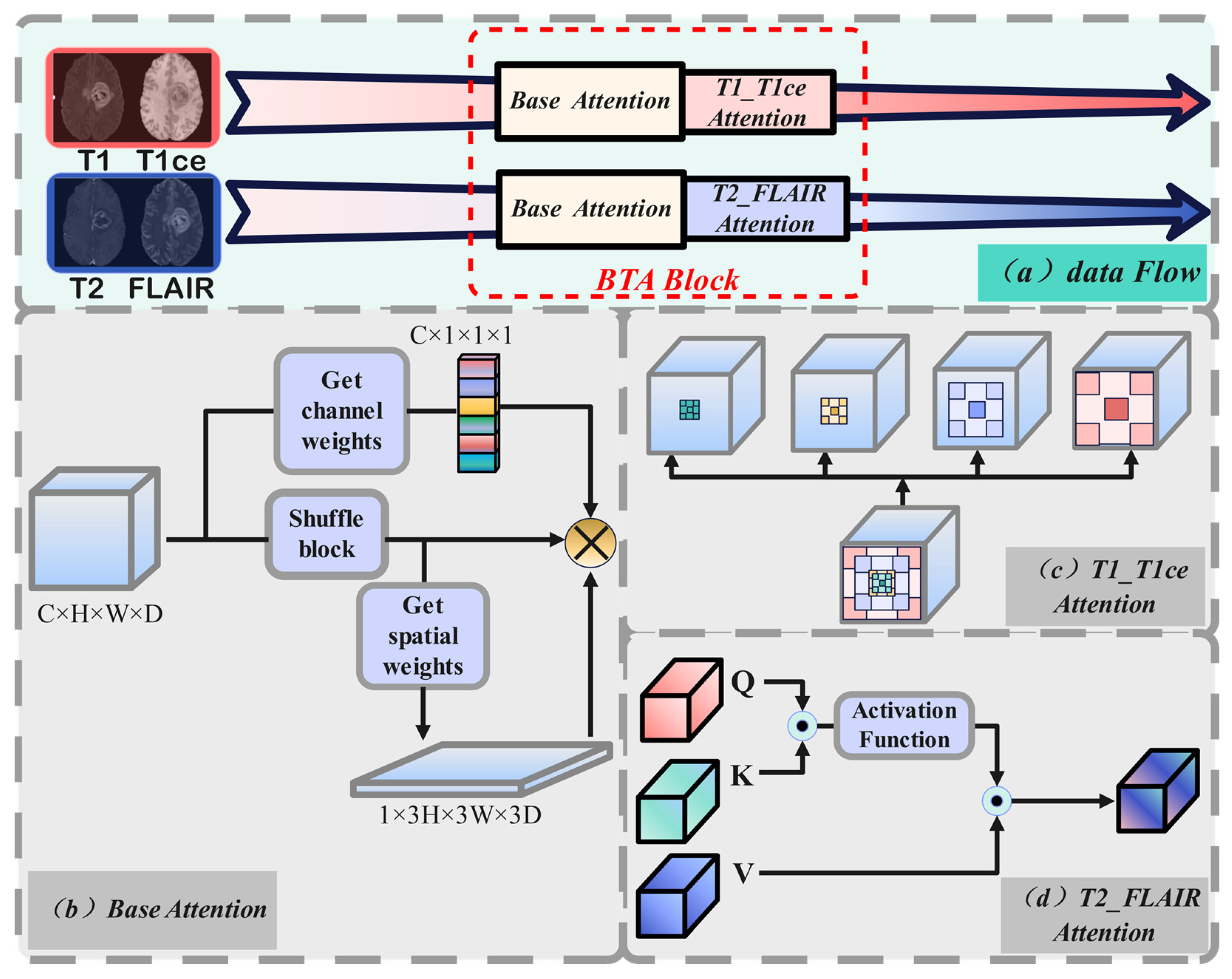
Unlike the conventional encoder, the grouped encoder processes distinct modality groups separately to exploit their complementary advantages. Images are grouped into the four independent MRI modalities (T1, T1ce, T2, and FLAIR) based on clinical knowledge before entering the grouped encoder. Grouping is typically implemented via concatenation. The process mainly relies on base attention, T1_T1ce and T2_FLAlR Modality Group Attention which is called BTA. The feature processing workflow is shown in Figure 4.
The base attention integrates spatial and channel attention mechanisms with a shuffle block. Spatial attention weights directly enhance the model’s response to spatial features. Spatial attention weights are calculated as follows:
S W = G W ( c o n c a t ( A P x ,   M P x ) )
where x denotes the input, S W defines the spatial attention weight, A P and M P are average pooling and max-pooling, C S stands for convolution and sigmoid, and G W represents obtaining feature Spatial weights through 3 × 3 × 3 convolutions with padding 1 and activation function sigmoid.
In the base attention mechanism, the shuffle block accelerates feature interaction within groups. It uses modality-shared features to dynamically highlight task-relevant features and suppress noise. The shuffle module can be described as follows:
s = s h u f f l e ( x )
where x denotes the input, s represents channel shuffle output, and s h u f f l e ( · ) means channel shuffling operation.
Channel attention weights, by adaptively learning each channel’s significance, enhance the model’s understanding of inter-channel relationships and feature representation capabilities. They can be described as follows:
C W = L N S ( L N R ( G P ( x ) ) )
where x and C W are the input and channel attention weight, respectively. L N S denotes Linear and activation function sigmoid, L N R represents Linear and ReLU, and G P is global average pooling.
To more precisely obtain the features fused within groups, the base attention mechanism T can be represented as follows:
T = s × S W × C W
where T denotes the output of base attention, s represents channel shuffle output, S W mean spatial attention weight, and C W is the channel attention weight.
In addition, to further enhance feature extraction, we added T1_T1ce and T2_FLAIR attention mechanisms to the T1_T1ce modality group and T2_FLAIR modality group. The former focuses on extracting multi-scale information, and the latter on global information. T1_T1ce attention mechanisms can be represented as follows:
A T 1 _ T 1 c e = C o n v ( c o n c a t ( A t r o u s ( A P T , θ ) ) )
where T denotes the input feature, and A T 1 _ T 1 c e represents the output result. A t r o u s indicates the Atrous Convolution operation with rate θ ∈ {2, 3, 4, 6}. AP stands for average pooling, and C o n v represents a convolution with 1 × 1 × 1 kernel, stride 1, and padding 1.
T2_FLAIR attention mechanisms can be represented as follows:
A T 2 _ F L A I R = γ × b m m ( C o n v T ,   s i g m o i d ( b m m ( C o n v ( T ) , C o n v ( T ) C o n v ( T ) T ) ) + T )
where T is the input feature, and A T 2 F L A I R is the output result. b m m denotes matrix multiplication, and C o n v represents a convolution with 1 × 1 × 1 kernel, stride 1, and padding 0. γ is a learnable parameter updated during model training to optimize results.

3.3. Mixer

In the GMD architecture, the mixer, a core component, is responsible for fusing and re-extracting features from the four modalities: T1, T1ce, T2, and FLAIR. Usually, feature extraction across different modalities relies on simple interaction strategies like channel concatenation [54] or parameter sharing [55]. While channel concatenation can form a more comprehensive and richer feature representation, it is prone to redundant information in feature maps. On the other hand, parameter sharing can easily establish associations between data and complement information but may ignore the unique features of each modality.
To more effectively integrate features from different modalities, we innovatively combine channel concatenation and parameter sharing, and introduce weight acquisition and feature shuffling operations to enhance feature crossing and fusion. Channel concatenation is performed during the input phase of the FMA block. Parameter sharing is used in the B and C feature extraction operation in Figure 5. During the preliminary processing stage in the grouped encoder, features are only collected between grouped modalities without in-depth feature extraction for each of the four modalities. Therefore, the mixer’s secondary feature extraction is a crucial supplement to the features extracted by the previous grouped encoder.
The mixer composition is FMA block, which is shown in Figure 5. Typically, the mixer first concatenates the T1_T1ce modality group and the T2_FLAIR modality group at the channel and extracts interaction features. To integrate channel and spatial features, it processes features separately at the channel and spatial level, ensuring feature commonality while leveraging the information differences between modalities. Next, it uses feature shuffling to better capture the complex relationships in multi-modality data, further enhancing feature diversity and richness.
The first step of channel-wise concatenation and interaction feature extraction can be described as follows:
F R = C o n v ( D W C o n v ( C o n v ( c o n c a t ( A T 1 _ T 1 c e , A T 2 _ F L A I R ) ) ) )
where C o n v denotes 1 × 1 × 1 convolutions, and D W C o n v represents 3 × 3 × 3 Depthwise Convolution. A T 1 _ T 1 c e and A T 2 _ F L A I R denote the T1_T1ce group and T2_FLAIR group feature map, respectively.
The feature split along the channel dimension can be described as follows:
F R 1 , F R 2 = s p l i t ( F R , 2 )
where s p l i t ( ) represents the channel split operation. F R 1 and F R 2 represent the output features of channel split operations.
The separate processing of channel features and spatial features fusion can be described as follows:
F c f = s ( c o n c a t L N S L N R G P F R 1 × F R 1 , G W ( c o n c a t ( A P F R 2 , M P ( F R 2 ) ) × F R 2 )
where F c f   is the output feature of the FMA block, and G P denotes the global average pool. L N S and L N R indicate Linear Sigmoid and Linear ReLU, respectively. G W is the get weight. The weight acquisition adopts convolution and sigmoid. M P and A P are max-pooling and average pooling, respectively. s is channel shuffle.

3.4. Decoder

The decoder aims to restore image details crucial for precise segmentation. In the first decoder layer (the bottom layer), features are small-sized yet rich in semantic information. Integrating features across scales endows the first layer with both local details and global semantics. MAA achieves this via a multi-scale feature strategy along each feature axis. Consequently, we implement MAA at the start of the first layer to capture global semantic information while integrating detailed features. The remaining decoder layers then progressively restore image details through upsampling and skip connections, ultimately achieving precise segmentation. A diagram of the MAA block is shown in Figure 6.
MAA can be described as follows:
A M A A = Z d ( C o n v c o n c a t A t r o u s A P x , θ , h w d )
where x denotes the output of the grouped encoder, and A M A A represents the result after processing by MAA. A t r o u s stands for Atrous Convolution with rate θ ∈ {1, 2, 3, 4}. A P is average pooling, and C o n v represents convolution with 1 × 1 × 1 kernel, stride 1, and padding 1. Z d indicates Formula (6), h is the column, w the row, and d the depth.

4. Experiments

4.1. Datasets and Preprocessing

In this study, we employ the BraTS 2018 [56,57,58] and BraTS 2021 [59] datasets, which are publicly available and can be utilized free of charge for training brain tumor segmentation algorithms. The training datasets were meticulously annotated by board-certified neuroradiologists who manually delineated the brain tumor regions, ensuring high-quality ground truth for model training. However, the validation dataset annotations were not directly accessible, and the segmentation results were validated online via the BraTS website (https://www.synapse.org/) (accessed on 25 March 2025).
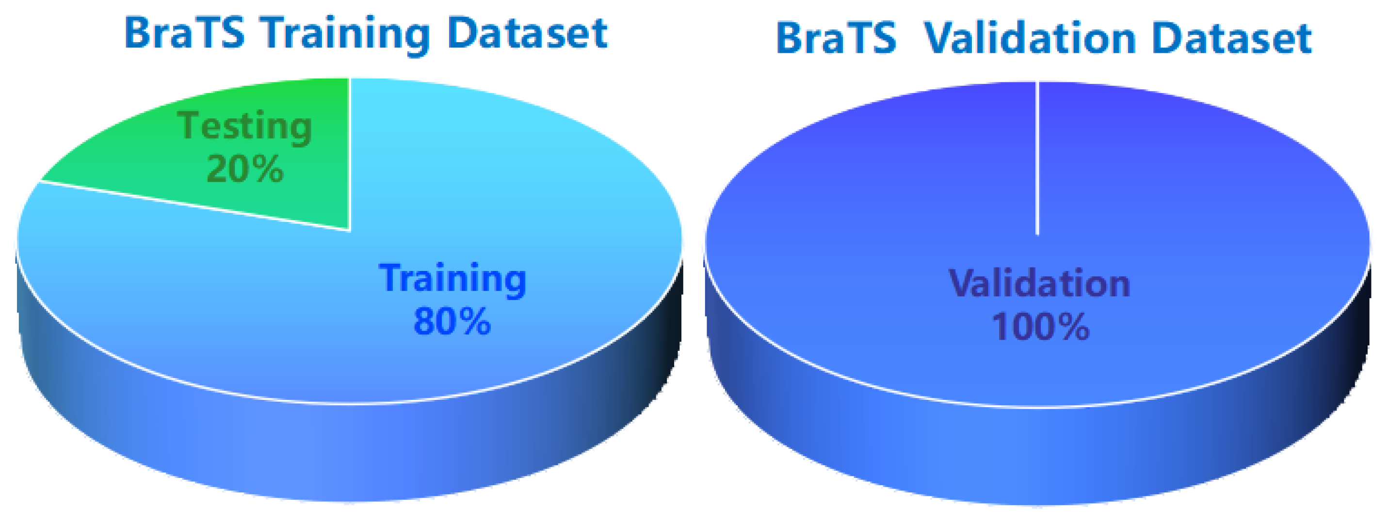
For experimental setup, we adopted a training strategy where 80% of the training dataset was allocated for model training, while the remaining 20% was reserved for model testing to evaluate its generalization capability, as shown in Figure 7. During the preprocessing phase, SimpleITK was employed for efficient image processing, and z-score normalization was applied to standardize the data, ensuring consistent intensity distributions across different scans. To minimize the impact of irrelevant background information and focus on the regions of interest, the images were randomly cropped to size of 128 × 128 × 128. This cropping strategy not only reduced computational overhead but also helped the model concentrate on the tumor and its surrounding tissues.
In the data augmentation stage, we implemented a series of geometric and intensity transformations to enhance the diversity of the training data and improve the model’s robustness. Specifically, we incorporated random rotations within the range of −30 to 30 degrees to simulate different viewing angles of the brain scans. Gaussian noise with a standard deviation of 0.1 was added to mimic real-world imaging noise conditions. Additionally, blurring with intensities ranging from 0.5 to 1 was applied to simulate varying degrees of image blur that might occur during acquisition. Finally, gamma correction values between 0.7 and 1.5 were used to adjust the intensity distributions, simulating different imaging contrasts. These augmentation techniques collectively aimed to expose the model to a wide variety of data variations, thereby enhancing its ability to generalize to unseen cases and improving its overall performance in brain tumor segmentation tasks.

4.2. Implementation Details and Loss Function

In the network implementation, we utilized Python version 3.8.10 and PyTorch version 1.10.0 as the primary development and deep learning frameworks. The training process was accelerated by an NVIDIA GeForce RTX 4090 GPU (Manufactured by Nvidia Corporation, Santa Clara, CA, USA) equipped with 24 GB of memory, while a single Intel(R) Xeon(R) Gold 6430 CPU was employed to handle background processes and data management tasks. We initiated the training with a learning rate of 1 × 10⁻⁴ and adopted a batch size of 1 considering the complexity of the model and the high dimensionality of medical images. The Ranger [60] optimizer was implemented to leverage the benefits of both Adam and LookAhead optimization algorithms, facilitating faster convergence and enhancing model stability. The Ranger optimizer solves Adam’s instability problem through the RAdam part, ensuring the stability of the training process. The LookAhead part reduces the need for tuning a large number of hyperparameters through dynamic speed adjustment strategies, achieving faster convergence with minimal computational overhead and improving the search efficiency of the global optimal solution. The implementation details are presented in Table 1.
For the loss function, we implemented the Soft Dice loss [61], which is particularly effective in addressing class imbalance issues inherent in medical image segmentation tasks. Unlike traditional pixel-wise loss functions that focus solely on classification accuracy, the Soft Dice loss calculates the similarity between the predicted and ground-truth segmentation masks using the Dice coefficient. This approach ensures that the model pays more attention to the accuracy of the segmentation results, especially for minority classes such as tumor regions that occupy a small proportion of the entire image. By computing the Dice loss separately for each class and then averaging them, the Soft Dice loss prevents the dominant majority classes from overshadowing the minority classes during the optimization process. Consequently, the model is guided to learn features that are more representative and discriminative for all classes, leading to improved segmentation performance, particularly for the less frequent but clinically significant brain tumor regions.

4.3. Evaluation Metrics

To assess the segmentation results, we employed two widely used metrics: Dice scores [62] and the Hausdorff Distance (HD) [63,64]. The Dice score evaluates the overlap between the predicted segmentation and the ground truth by comparing the area of overlap to the total area of both the predicted and true regions. It is calculated as follows:
D i c e = ( 2 × Y P r e v a l ) ( 2 × Y M a n v a l ) Y P r e v a l + Y M a n v a l
where Y P r e v a l represents the predicted segmentation and Y M a n v a l represents the ground truth. This metric ranges from 0 to 1, with higher values indicating better segmentation accuracy.
The HD, on the other hand, measures the maximum distance between the predicted and true segmentations, providing a more stringent assessment of the segmentation boundary accuracy. It is determined by calculating the distances between the boundaries of the predicted and ground truth segmentations. A smaller HD value signifies closer alignment between the predicted and true boundaries, demonstrating more precise segmentation results.
H D = m a x { s u p t T i n f p P   d t , p , s u p p P i n f t T   d ( t , p ) }
where t represents the true region boundary, p represents the predicted segmentation boundary, and d ( t , p ) stands for the distance between t and p . s u p denotes the supremum, and i n f is the infimum.

5. Results and Analysis

The experimental procedure of this paper is shown in Figure 8.

5.1. Complete Modality

5.1.1. Comparison with Methods in Complete Modality

In this paper, we compare the GMDNet with advanced segmentation methods on the BraTS 2018 and BraTS 2021 datasets. Table 2 compares GMDNet with 10 brain tumor segmentation networks on the BraTS 2018, including two from 2024, two from 2023, two from 2022, and four classic networks. MSFR-NET and RFTNet are modality-fusion-based brain tumor segmentation networks. Compared to common 3D UNet, its variants, Transformer, Transformer + CNN, and multi-modality fusion networks, GMDNet excels by fully leveraging the multi-modality characteristics of brain tumor MRI data, which also proves the advantage of the Grouped Encoder-Mixer-Decoder architecture. GMDNet shows excellent segmentation performance in all three brain tumor subregions and has the highest average Dice score among all compared networks, which reveals its strong performance in brain tumor segmentation tasks.
Table 3 shows the comparison between GMDNet and 11 state-of-the-art models on the BraTS 2021 dataset to evaluate its performance. The number of comparison networks was two in 2024, two in 2023, and two in 2022. We assess the network’s performance using WT, TC, ET, average Dice, and HD95. The results are presented in tabular form. GMDNet achieves a higher average Dice score (87.42%) than the 11 networks. The Dice results for WT, TC, and ET are 91.87%, 87.25%, and 83.16%, respectively. Our method also has the lowest average HD95 value of 10.55, outperforming the compared segmentation methods.
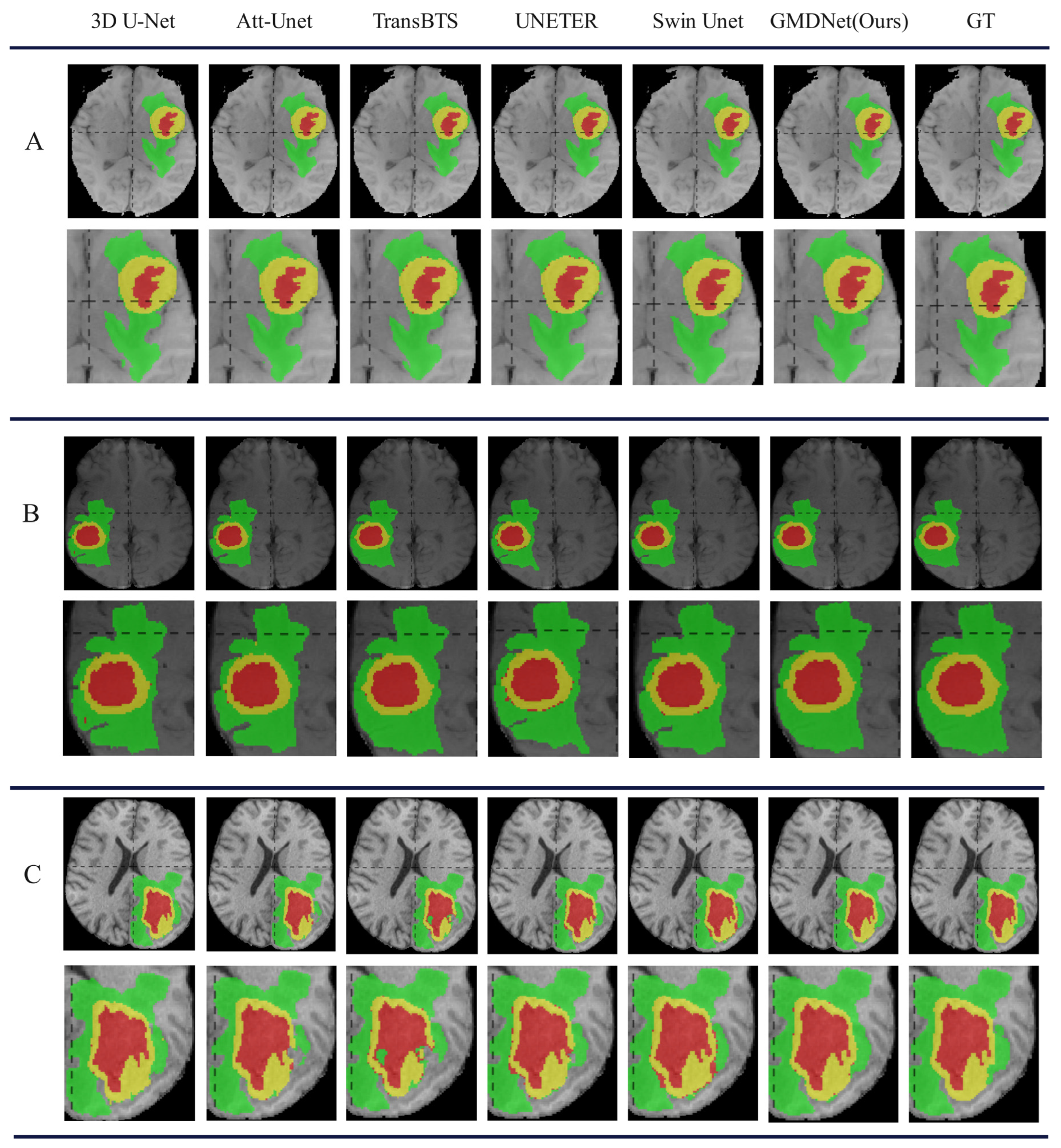
To validate the segmentation results, we randomly selected three MRI cases from the BraTS 2021 for evaluation. The compared models, from left to right, include 3D UNet, Att-Unet, TransBTS, UNETR, Swin Unet, and GMDNet, with the manual segmentation results on the right. As shown in Figure 9, the results of GMDNet are closer to the ground truth than compared methods, highlighting its effectiveness. In addition, we conducted paired t-test experiments to verify that the improvement in GMDNet was statistically significant. The statistical test results are shown in Table 4.

5.1.2. Ablation Study of Each Component in GMDNet

GMDNet contains three attention modules: BTA (Base Attention and T1_T1ce and T2_FLAlR Modality Group Attention), MAA (Multi-Scale Axial Attention), and FMA (Feature Mixer Attention). Additionally, to accelerate training and convergence, DP (Deep Supervision Mechanism) is used. For systematic evaluation of GMDNet, ablation studies on these components are conducted. Here, A is the baseline based on the traditional U-Net. Experiment B groups MRI modalities in the encoder stage of A. Experiments C, D, and E add the BTA, FMA, and MAA modules to group B. Experiment F introduces all three modules at once. Results are shown in Table 5 and Figure 10.
The experimental results show that after grouping the modalities, the Dice values for WT and TC in experiment B increased by 2.1% and 3.04%, respectively, compared to experiment A. This indicates that effective modality grouping helps in feature extraction. In experiment C, where only the fusion module was used based on experiment A, the Dice values for WT, TC, ET, and the average increased by 2.25%, 4.51%, 6.44%, and 4.4%, respectively, compared to experiment A. This shows that the FMA module, by combining parameter sharing and feature map channel concatenation, can promote the fusion of information between different modalities and supplement the encoder features through attention mechanisms. In experiment D, where BTA was added to experiment B, the Dice values for WT, TC, ET, and the average segmentation area increased by 1.69%, 3.52%, 6.69%, and 3.97%, respectively, compared to experiment A. This demonstrates that BTA enhances the network’s feature extraction for different modalities. In experiment E, where the MAA module was added to experiment B, the Dice values for WT, TC, ET, and the average increased by 0.36%, 3.42%, 5.14%, and 2.98%, respectively. Experiment F shows that combining BTA, FMA, and MAA achieves an average Dice of 87.05%. Finally, introducing the deep supervision mechanism (Experiment G) leads to small improvement in segmentation results.

5.1.3. Research on GMD Architecture

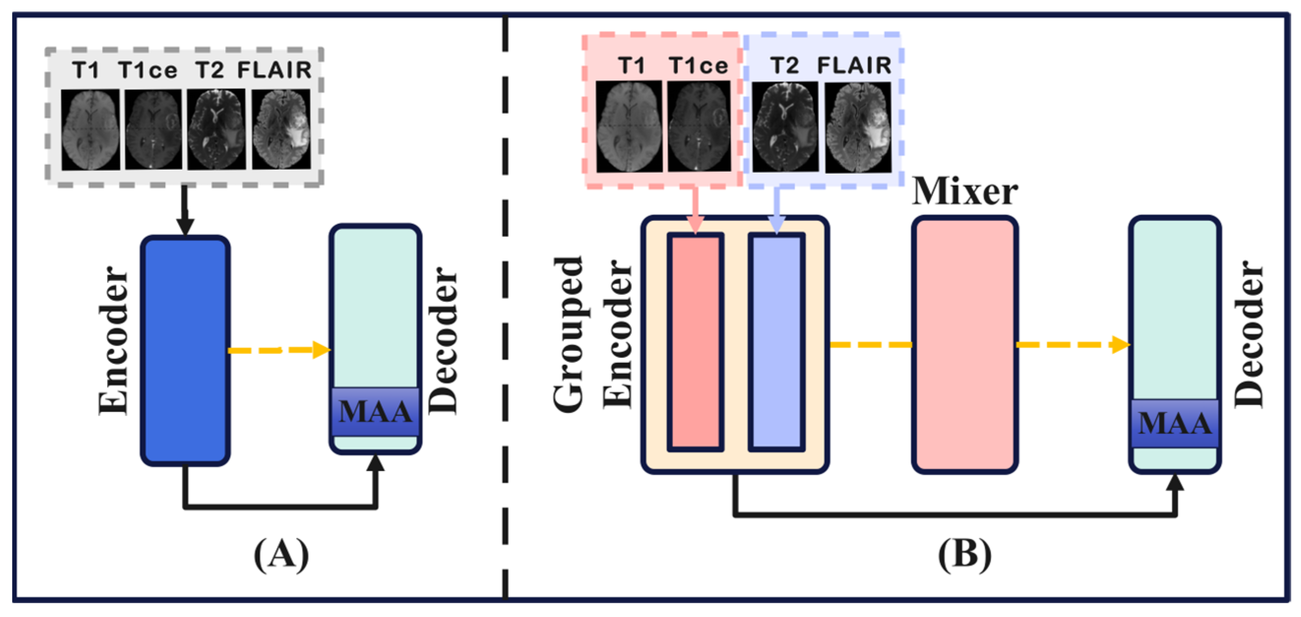
In Section 5.1.2, sufficient ablation experiments were conducted on the GMDNet. In addition, we also studied the segmentation performance, FLOPs and Parameters of the GMD architecture. The experimental setup is shown in Figure 11, where (A) the MAA module is added to the traditional Encoder–Decoder architecture. (B) On the basis of (A), Grouped Encoder and Mixer are added. The experimental results are shown in Table 6. From the experimental results, it can be seen that Experiment B increased FLOPs by 243.55 G and decreased Parameter by 12.712 M compared to Experiment A. The Dice values for WT, TC, ET, and the average segmentation area increased by 1.96%, 1.33%, 0.75%, and 1.34%. The experimental results demonstrate the advantages of GMD architecture in terms of parameters and segmentation performance.

5.2. Incomplete Modality

5.2.1. Comparison with Methods in Incomplete Modality

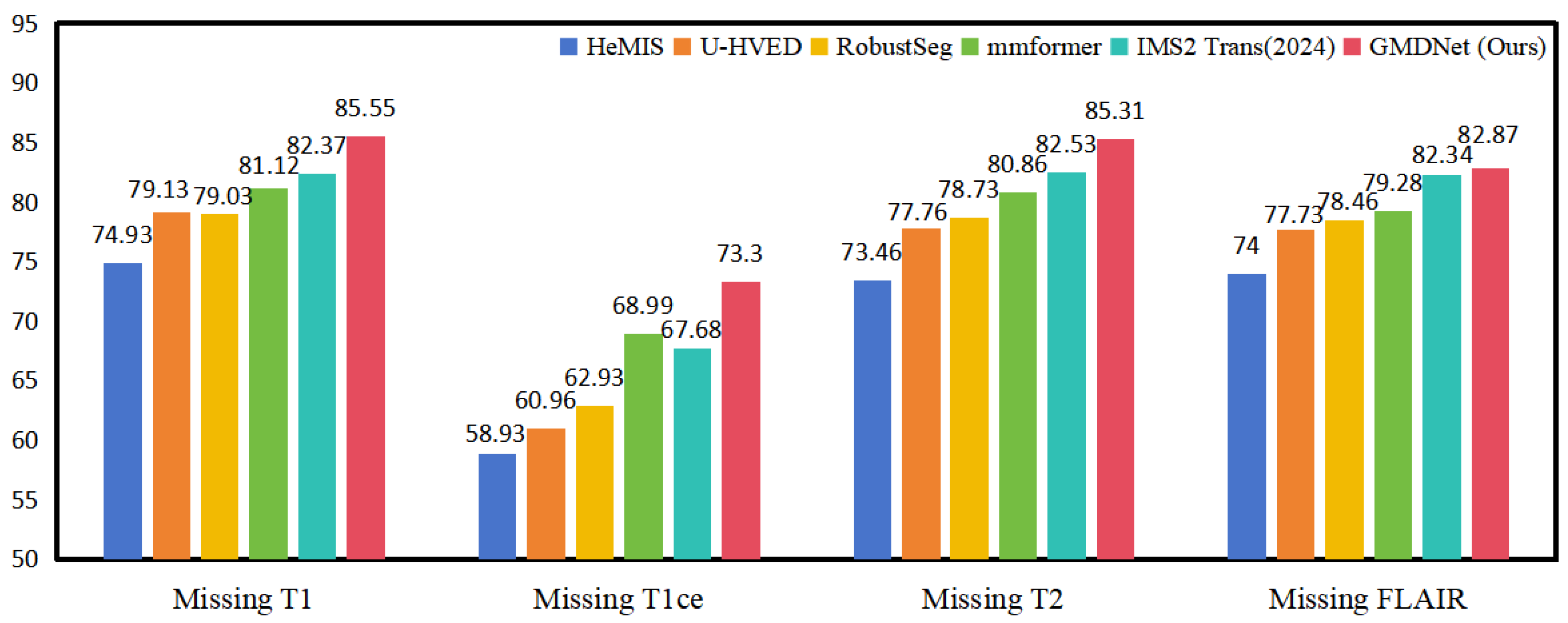
While the model under consideration achieved remarkable performance with complete modality, incomplete modality is common in clinical settings. We conducted experiments to evaluate the Grouped Encoder-Mixer-Decoder architecture’s segmentation performance under incomplete modality. We tested cases with one incomplete modality and compared results with five networks: HeMIS [49], U-HVED [50], RobustSeg [78], mmformer [67] and IMS2 Trans [51]. The results are shown in Table 7 and Figure 12. Since most incomplete modality studies use the BraTS 2018 dataset, we also used it for consistency. The results show that GMDNet maintains excellent performance even with incomplete modality, outperforming the four comparison networks. In cases of missing T1, T1ce, T2, and FLAIR, GMDNet’s average Dice scores reached 85.54%, 73.3%, 85.31%, and 82.87%, respectively. Compared to the advanced IMS2 Trans method, GMDNet achieved average Dice score improvements of 3.18%, 5.62%, 2.78%, and 0.53% in the respective incomplete modality. Notably, GMDNet showed the best performance when T2 was missing.
The experimental results imply the proposed GMD architecture’s superiority in brain tumor segmentation. Its effectiveness mainly comes from the grouped encoder and mixer component. The former can learn information from inter-modality within the same group under incomplete modality, thus supplementing relevant information. The latter improves the final segmentation results through cross-modality group information fusion. GMDNet shows the most significant effects in the TC and ET regions. Compared with common tumor segmentation methods for incomplete modality, the Grouped Encoder-Mixer-Decoder structure achieves better segmentation performance in brain tumor segmentation under incomplete modality.

5.2.2. Study on Single Modality

In prior evaluation experiments, we explored segmentation with incomplete modality and found that removing a modality affects the results in specific ways. To study the role of each modality in brain tumor segmentation, we conducted experiments using GMDNet with single modality. As shown in Figure 13, we used one of the four modalities from the BraTS 2021 as input to GMDNet for segmentation.
Table 8 shows the experimental results for each MRI modality. T1 has the lowest segmentation results for all three subregions (WT, TC, and ET) compared to the other modalities. T1ce has the lowest segmentation results for WT at 80.19%, but the highest for ET and TC at 78.53% and 79.47%, respectively. T2 does not have the highest segmentation results for any subregion, but its results are close to the highest. FLAIR plays a key role in segmenting the WT region, achieving 91.04%, nearly matching the segmentation results of the tumor edema region under complete modality.
Analyzing the brain tumor segmentation results for each MRI modality reveals their correlation with the three tumor subregions (WT, TC, and ET). The T1 modality shows body structure but only roughly displays the edema/infiltrated tissues around the tumor, resulting in unclear tumor boundaries and low correlation with all three subregions. In incomplete modality segmentation, the average segmentation results (WT, TC, and ET) without T1 are higher than with the other modalities. T1ce, obtained via MRI after contrast agent administration, highlights brain areas with more blood, making TC and WT more visible. T2-weighted images have signals related to water content: high intensity for water-rich tissues (e.g., fluids, tumors) and low intensity for water-poor tissues (e.g., bones, fibrous tissues). T2-weighted images are better for observing tumor edema, locating tumors, and determining their size, showing strong correlation with WT. FLAIR suppresses the high CSF (Signal of Cerebrospinal Fluid) using an MRI fluid attenuation inversion recovery sequence, making CSF appear darker and adjacent lesions brighter. FLAIR combines T1 and T2, suppresses CSF’s high signal, and is less effective for TC and ET segmentation but provides tumor location and edema–boundary information, giving it the highest correlation with WT. The correlations between modality sequences and brain tumor subregions (WT, TC, and ET) are shown in Table 9.
The experiments with MRI modalities confirm the rationality of grouping T1 and T1ce together, and T2 with FLAIR. Each modality group has consistent information, while different groups offer complementary information. Using tailored feature-extraction methods for each group enriches the features, improving brain tumor segmentation performance.

5.3. Reuse Modality Strategy

To address brain tumor segmentation with incomplete modality, we innovatively proposed leveraging existing modalities to improve segmentation when one is missing. We conducted experiments on the BraTS 2021 to explore the effectiveness of different modalities in compensating for missing ones.

5.3.1. Study on Reuse Modality Performance of Missing T1

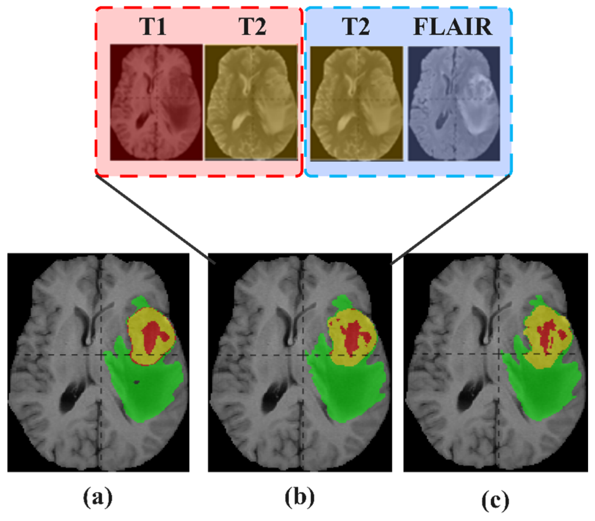
As prior studies have shown, T1 is weakly correlated with WT, TC, and ET in brain tumor segmentation. Thus, its absence has the least impact on segmentation results, a finding also supported by the incomplete modality experiments, which revealed the highest segmentation accuracy when T1 was missing. Using the GMD architecture for brain tumor segmentation, we conducted reuse modality experiments in the absence of T1. Results indicate that reusing T1ce slightly improves the Dice scores for WT and TC by 0.09% and 0.33%, respectively, but decreases ET segmentation by 0.6%. Reusing T2 causes a 1% and 0.59% drop in TC and ET segmentation, respectively, yet WT improves by 0.05%. The most significant enhancement comes from reusing FLAIR, which boosts segmentation results for WT, TC, and ET by 0.18%, 0.03%, and 1.9%, respectively, with an average Dice increase of 0.7%. This makes FLAIR the best choice for compensating for missing T1, as its imaging combines T1 and T2, retaining information from T1. FLAIR and T1ce can assist the network in segmenting the ET and TC regions within the group, as can also be seen from the experimental results. Consequently, reusing FLAIR achieves an average result of 87.17%, just 0.3% less than complete modality segmentation. The reuse results are shown in Table 10. The reuse effect is shown in Figure 14, and it can be seen from the same category that the reuse modality strategy significantly improves the segmentation results of the missing T1 for the NCR region.

5.3.2. Study on Reuse Modality Performance of Missing T1ce

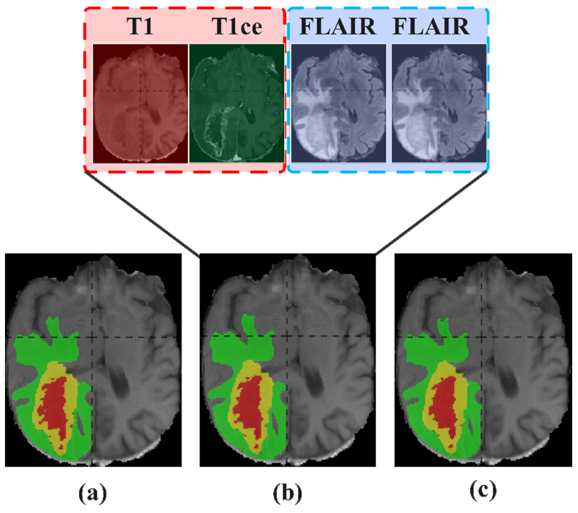
When T1ce is missing, the segmentation results for TC and ET drop significantly, lowering the average Dice score. Reusing T1 boosts segmentation results for WT, TC, and ET by 1.05%, 0.47%, and 2.63%, respectively. Reusing T2 also enhances results, increasing the scores for WT, TC, and ET by 1.02%, 1.12%, and 3.19%, respectively. Reusing FLAIR offers little improvement in this case, with WT increasing by 0.79%, ET by 1.34%, but TC dropping by 1.02%. Among these, reusing T2 provides the most significant boost, raising the average Dice score by 1.78% compared to when T1ce is missing. This is likely because T2 offers unique information about the tumor core and enhanced tumor, which T1 and FLAIR do not fully provide. Although reuse modality improves segmentation when T1ce is missing, results still lag behind those obtained with all modalities, as the key information about TC and ET in T1ce cannot be fully replicated by the remaining modalities. Table 11 shows the reuse results.
The reuse effect is shown in Figure 15. From the segmentation result graph, it can be seen that reusing T2 has improved the segmentation performance of ET and TC in the absence of T1ce, but there is still a gap in the segmentation results from the complete modality, which is consistent with results of Dice.

5.3.3. Study on Reuse Modality Performance of Missing T2

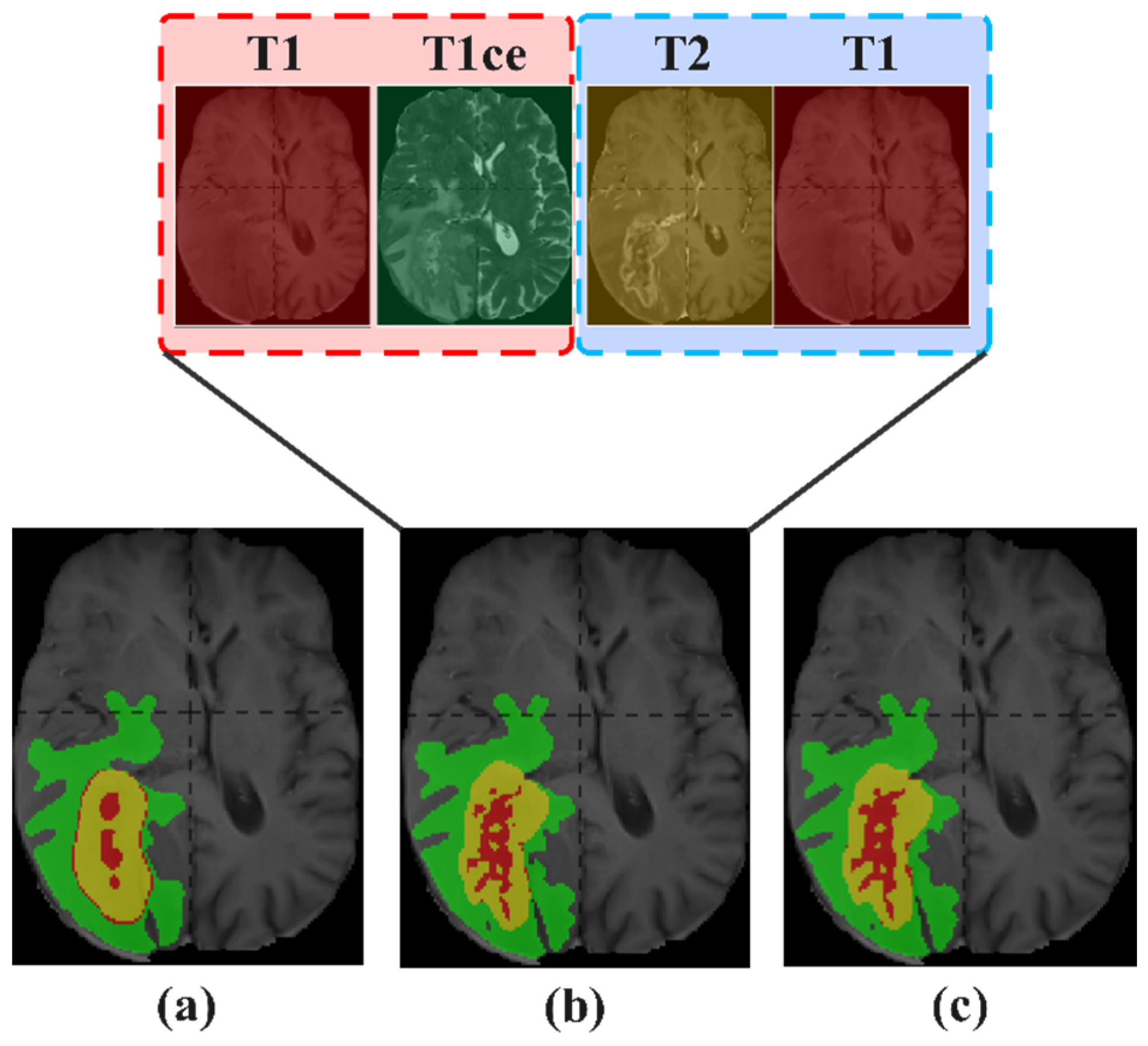
The absence of T2 has limited impact on WT, TC, and ET due to the strong correlation of T2 and FLAIR with the tumor edema region. Reusing T1 improves segmentation results for WT and ET by 0.11% and 1.11%, respectively, but decreases TC by 0.19%. Reusing T1ce reduces segmentation effects for WT and TC by 0.21% and 0.11%, respectively. Reusing FLAIR enhances results for WT, TC, ET, and the average Dice by 0.16%, 0.66%, 0.53%, and 0.45%, respectively. In cases of missing T2, reusing FLAIR is most effective for brain tumor segmentation due to its strong correlation with WT. Additionally, reusing FLAIR results in two FLAIR sequences, and since FLAIR combines T1 and T2 modalities, TC performance improves significantly. However, while reusing T1 and T1ce yields a lower average Dice than reusing FLAIR, it provides greater improvement for ET. This is because in the T2_FLAIR group, the combination of T1, T1ce, and FLAIR offers more information for ET segmentation. The reuse results are shown in Table 12.
The reuse effect is shown in Figure 16. From the figure, it can be observed that the segmentation result of missing T2 is very close to the complete modality, with only slight differences. By reusing FLAIR, the segmentation result can be further supplemented to make it closer to the complete modality segmentation result.

5.3.4. Study on Reuse Modality Performance of Missing FLAIR

As previous experiments have shown, the absence of FLAIR significantly impacts overall segmentation. Reusing T1, T2, and T1ce notably boosts the average Dice by 3.68%, 3.42%, and 3.43%, respectively. Specifically, reusing T1 enhances the Dice scores for WT, TC, and ET by 2.88%, 4.98%, and 3.19%, respectively, while reusing T2 improves them by 2.82%, 5.15%, and 2.3%. Reusing T1ce provides the most significant improvement for ET, increasing its score by 3.3%. This is because T1ce and T2 in the T2_FLAIR modality group offer crucial information for enhanced tumor segmentation. When reusing T1, the T2_FLAIR group consists of T1 and T2, which, similar to FLAIR’s imaging principles, provides information close to that of FLAIR. However, despite these improvements, the segmentation results for WT, TC, and ET when reusing a modality is still lower than when FLAIR is present, indicating that information captured by FLAIR cannot be fully replicated by the remaining modalities, as shown in Table 13.
The reuse effect is shown in Figure 17. In terms of ED, ET, and NCR, the ED region in the incomplete modality is basically the same as that in the complete modality, but there are still slight differences. NCR has the largest gap with the complete modality, followed by ET. However, NCR and ET play an extremely important role in brain tumor segmentation, which is a valuable basis for neuroradiologists to accurately diagnose. Segmentation performance under incomplete modality will affect their diagnosis. By reusing a modality, the segmentation results of incomplete modality can be made closer to complete modality.

5.3.5. Summary of Reuse Modality Strategy

The above experimental results demonstrate the effectiveness of the reuse modality strategy, which improves the segmentation results for all incomplete modality cases. Figure 18 presents the average Dice scores of the four modalities (T1, T1ce, T2, FLAIR) under incomplete modality, complete modality, and the reuse modality strategy. It shows that reuse modality with GMDNet mitigates the impact of incomplete modality to varying extents. Specifically, the T1 reuse strategy achieves 87.17% (within 0.3% of the complete modality result). Moreover, reusing modalities in the absence of FLAIR yields the most significant improvement, with an average Dice increase of 3.68% compared to the scenario without FLAIR.

6. Discussion and Conclusions

In this paper, a GMD architecture (Grouped Encoder-Mixer-Decoder) is proposed to enhance information interaction between different modalities and complement modality features, improving brain tumor MRI image segmentation. We developed GMDNet based on this architecture and introduced several modules to boost its performance: BTA (Base Attention and T1_T1ce and T2_FLAlR Modality Group Attention), MAA (Multi-Scale Axial Attention), and FMA (Feature Mixer Attention). Segmentation experiments on the BraTS 2018 and BraTS 2021 databases show that GMDNet outperforms other compared networks. On BraTS 2018, it achieves Dice scores of 91.21% for WT, 87.11% for TC, 80.97% for ET, and average Dice of 86.43%. On BraTS 2021, the results are 91.87% for WT, 87.25% for TC, 83.16% for ET, and average Dice of 87.42%. The ablation experiment results demonstrated the effectiveness of BTA, MAA, and FMA. In addition, it has been demonstrated that grouped modality and mixed strategy play an important role in brain tumor segmentation.
GMDNet excels not only in complete modality but also in incomplete modality. Incomplete modality experiments reveal that T1ce is most correlated with TC and ET, while T2 and FLAIR are closely related to WT. T1 shows weaker correlations. Missing T1ce has the most significant impact on segmentation results, while missing T1 has the least. To address performance drops in incomplete modality, we propose a reuse modality strategy. Experiments show that reusing T1 when FLAIR is missing improves results by 2.88% for WT, 4.98% for TC, 3.19% for ET, and 3.68% for average Dice. For the four types of incomplete modality, the segmentation results can be improved through the reuse modality strategy. The reuse results are closer to complete modality performance.

7. Limitations and Future Perspectives

In conclusion, GMD architecture offer superior brain tumor MRI image segmentation performance, even in incomplete modality. This work provides valuable insights for clinical applications, potentially reducing patient diagnosis time and costs. However, challenges like data quality in real clinical settings remain, prompting future research to further optimize network structures and improve segmentation performance. There may be potential overfitting and computational complexity issues in this study. In addition, it is necessary to conduct further research on the computational cost and parameter quantity of segmentation networks, so that they can be more widely applied in clinical diagnosis, and further study the reuse modality strategy to improve the segmentation performance of the architecture in incomplete modality.

Author Contributions

Conceptualization, B.G.; Methodology, B.G. and P.Y.; Software, P.Y. and R.Z.; Data Curation, C.H.; Writing—Original Draft, P.Y.; Writing—Review and Editing, B.G. and P.Y. All authors have read and agreed to the published version of the manuscript.

Funding

This research received no external funding.

Data Availability Statement

Publicly available datasets were analyzed in this study. The dataset can be found in the BraTS 2018 dataset: https://www.med.upenn.edu/sbia/brats2018/data.html (accessed on 25 March 2025). Datasets released to the public were analyzed in this study. The BraTS 2021 dataset can be found through the following link: https://www.med.upenn.edu/cbica/brats2021/#Data2 (accessed on 25 March 2025).

Conflicts of Interest

The authors declare no conflicts of interest.

References

  1. Kleihues, P.; Burger, P.C.; Scheithauer, B.W. The new WHO classification of brain tumours. Brain Pathol. 1993, 3, 255–268. [Google Scholar] [CrossRef] [PubMed]
  2. Rice, J.M. Inducible and transmissible genetic events and pediatric tumors of the nervous system. J. Radiat. Res. 2006, 47, B1–B11. [Google Scholar] [CrossRef] [PubMed]
  3. Persaud-Sharma, D.; Burns, J.; Trangle, J.; Sabyasachi, M. Disparities in brain cancer in the United States: A literature review of gliomas. Med. Sci. 2017, 5, 16. [Google Scholar] [CrossRef] [PubMed]
  4. Giese, A.; Westphal, M. Glioma invasion in the central nervous syste. Neurosurgery 1996, 39, 235–252. [Google Scholar] [CrossRef]
  5. Schneider, T.; Mawrin, C.; Scherlach, C.; Skalej, M.; Firsching, R. Gliomas in adult. Dtsch. Ärzteblatt Int. 2010, 107, 799–808. [Google Scholar] [CrossRef]
  6. Khalighi, S.; Reddy, K.; Midya, A.; Pandav, K.B.; Madabhushi, A.; Abedalthagafi, A. Artificial intelligence in neuro-oncology: Advances and challenges in brain tumor diagnosis, prognosis, and precision treatmen. NPJ Precis. Oncol. 2024, 8, 80. [Google Scholar] [CrossRef]
  7. Iqbal, S.; Khan, M.U.G.; Saba, T.; Rehman, A. Computer-assisted brain tumor type discrimination using magnetic resonance imaging feature. Biomed. Eng. Lett. 2018, 8, 5–28. [Google Scholar] [CrossRef]
  8. Najjar, R. Clinical applications, safety profiles, and future developments of contrast agents in modern radiology: A comprehensive review. iRADIOLOGY 2024, 2, 430–468. [Google Scholar] [CrossRef]
  9. Farhan, A.S.; Khalid, M.; Manzoor, U. XAI-MRI: An ensemble dual-modality approach for 3D brain tumor segmentation using magnetic resonance imagin. Front. Artif. Intell. 2025, 8, 1525240. [Google Scholar] [CrossRef]
  10. Howarth, C.; Hutton, C.; Deichmann, R. Improvement of the image quality of T1-weighted anatomical brain scans. Neuroimage 2006, 29, 930–937. [Google Scholar] [CrossRef]
  11. Lei, Y.; Xu, L.; Wang, X.; Zheng, B. IFGAN: Pre-to Post-Contrast Medical Image Synthesis Based on Interactive Frequency GA. Electronics 2024, 13, 4351. [Google Scholar] [CrossRef]
  12. Liu, Z.; Wei, J.; Li, R.; Zhou, J. Learning multi-modal brain tumor segmentation from privileged semi-paired MRI images with curriculum disentanglement learnin. Comput. Biol. Med. 2023, 159, 106927. [Google Scholar] [CrossRef] [PubMed]
  13. Ferreira, V.M.; Piechnik, S.K.; Dall’Armellina, E.; Karamitsos, T.D.; Francis, J.M.; Choudhury, R.P.; Friedrich, M.J.; Robson, M.D.; Neubauer, S. Non-contrast T1-map** detects acute myocardial edema with high diagnostic accuracy: A comparison to T2-weighted cardiovascular magnetic resonanc. J. Cardiovasc. Magn. Reson. 2012, 14, 53. [Google Scholar] [CrossRef] [PubMed]
  14. Sati, P.; George, I.C.; Shea, C.D.; Gaitán, M.I.; Reich, D.S. FLAIR*: A combined MR contrast technique for visualizing white matter lesions and parenchymal veins. Radiology 2012, 265, 926–932. [Google Scholar] [CrossRef]
  15. Usuzaki, T.; Takahashi, K.; Inamori, R.; Morishita1, Y.; Shizukuishi1, T.; Takagi1, H.; Ishikur, M.; Obar, T.; Takase, K. Identifying key factors for predicting O6-Methylguanine-DNA methyltransferase status in adult patients with diffuse glioma: A multimodal analysis of demographics, radiomics, and MRI by variable Vision Transformer. Neuroradiology 2024, 66, 761–773. [Google Scholar] [CrossRef]
  16. Jiang, Z.; Capellán-Martín, D.; Parida, A.; Liu, X.; Ledesma-Carbayo, M.J.; Anwar, S.M.; Linguraru, M.G. Enhancing generalizability in brain tumor segmentation: Model ensemble with adaptive post-processing. In Proceedings of the 2024 IEEE International Symposium on Biomedical Imaging, Athens, Greece, 27–30 May 2024; pp. 1–4. [Google Scholar] [CrossRef]
  17. Liu, Z.; Ma, C.; She, W. A multi-plane 2D medical image segmentation method combined with transformers. In Proceedings of the International Conference on Remote Sensing, Mapping, and Image Processing (RSMIP 2024), Xiamen, China, 21 June 2024; pp. 721–727. [Google Scholar] [CrossRef]
  18. Çiçek, Ö.; Abdulkadir, A.; Lienkamp, S.S.; Brox, T.; Ronneberger, O. 3D U-Net: Learning dense volumetric segmentation from sparse annotation. In Proceedings of the Medical Image Computing and Computer-Assisted Intervention–MICCAI 2016: 19th International Conference, Athens, Greece, 17–21 October 2016; pp. 424–432. [Google Scholar]
  19. Bukhari, S.T.; Mohy-ud-Din, H. E1D3 U-Net for brain tumor segmentation: Submission to the RSNA-ASNR-MICCAI BraTS 2021 challenge. In Brainlesion: Glioma, Multiple Sclerosis, Stroke and Traumatic Brain Injuries, Proceedings of the International MICCAI Brainlesion Workshop, Virtual Event, 27 September 2021; Springer: Cham, Switzerland, 2021; pp. 276–288. [Google Scholar] [CrossRef]
  20. Jiao, C.; Yang, T.; Yan, Y.; Yang, A. Rftnet: Region–attention fusion network combined with dual-branch vision transformer for multimodal brain tumor image segmentatio. Electronics 2023, 13, 77. [Google Scholar] [CrossRef]
  21. Liu, X.; Song, L.; Liu, S.; Zhang, Y. A review of deep-learning-based medical image segmentation method. Sustainability 2021, 13, 1224. [Google Scholar] [CrossRef]
  22. Cai, L.; Gao, J.; Zhao, D. A review of the application of deep learning in medical image classification and segmentatio. Ann. Transl. Med. 2020, 8, 713. [Google Scholar] [CrossRef]
  23. Thakur, G.K.; Thakur, A.; Kulkarni, S.; Khan, N.; Khan, S. Deep learning approaches for medical image analysis and diagnosi. Cureus 2024, 16, e59507. [Google Scholar] [CrossRef]
  24. Rasool, N.; Bhat, J.I. Unveiling the complexity of medical imaging through deep learning approache. Chaos Theory Appl. 2023, 5, 267–280. [Google Scholar] [CrossRef]
  25. Mistry, J. Automated Knowledge Transfer for Medical Image Segmentation Using Deep Learnin. J. Xidian Univ. 2024, 18, 601–610. [Google Scholar]
  26. Sahiner, B.; Chan, H.P.; Petrick, N.; Wei, D.; Helvie, M.A.; Adler, D.D.; Goodsitt, M.M. Classification of mass and normal breast tissue: A convolution neural network classifier with spatial domain and texture image. IEEE Trans. Med. Imaging 1996, 15, 598–610. [Google Scholar] [CrossRef]
  27. Rawat, W.; Wang, Z. Deep convolutional neural networks for image classification: A comprehensive revie. Neural Comput. 2017, 29, 2352–2449. [Google Scholar] [CrossRef]
  28. Chen, L.; Li, S.; Bai, Q.; Yang, J.; Jiang, S.; Miao, Y. Review of image classification algorithms based on convolutional neural networks. Remote Sens. 2021, 13, 4712. [Google Scholar] [CrossRef]
  29. Weng, Y.; Zhou, T.; Li, Y.; Qiu, X. Nas-unet: Neural architecture search for medical image segmentatio. IEEE Access 2019, 7, 44247–44257. [Google Scholar] [CrossRef]
  30. Yasrab, R.; Gu, N.; Zhang, X. An encoder-decoder based convolution neural network (CNN) for future advanced driver assistance system (ADAS). Appl. Sci. 2017, 7, 312. [Google Scholar] [CrossRef]
  31. Zhang, J.; Luan, Z.; Qi, L.; Gong, X. MSDANet: A multi-scale dilation attention network for medical image segmentatio. Biomed. Signal Process. Control 2024, 90, 105889. [Google Scholar] [CrossRef]
  32. Nie, D.; Lu, J.; Zhang, H.; Adeli, E.; Wang, J.; Yu, Z.; Liu, L.Y.; Wang, Q.; Shen, D. Multi-channel 3D deep feature learning for survival time prediction of brain tumor patients using multi-modal neuroimages. Sci. Rep. 2019, 9, 1103. [Google Scholar] [CrossRef]
  33. Zucchet, N.; Orvieto, A. Recurrent neural networks: Vanishing and exploding gradients are not the end of the stor. Adv. Neural Inf. Process. Syst. 2024, 37, 139402–139443. [Google Scholar]
  34. Zhou, Z.; Rahman Siddiquee, M.M.; Tajbakhsh, N.; Liang, J. Unet++: A nested u-net architecture for medical image segmentation. In Deep Learning in Medical Image Analysis and Multimodal Learning for Clinical Decision Support Proceedings of the 4th International Workshop, DLMIA 2018, and 8th International Workshop, ML-CDS 2018, Granada, Spain, 20 September 2018; Held in Conjunction with MICCAI 2018; Springer: Cham, Switzerland, 2018; pp. 3–11. [Google Scholar] [CrossRef]
  35. Huang, X.; Deng, Z.; Li, D.; Yuan, X. Missformer: An effective medical image segmentation transformer. arXiv 2021, arXiv:2109.07162. [Google Scholar] [CrossRef]
  36. Jia, Q.; Shu, H. Bitr-unet: A cnn-transformer combined network for mri brain tumor segmentation. In Proceedings of the International MICCAI Brainlesion Workshop, Virtual Event, 27 September 2021; pp. 3–14. [Google Scholar] [CrossRef]
  37. Yu, M.; Han, M.; Li, X.; Wei, X.; Jiang, H.; Chen, H.; Yu, R. Adaptive soft erasure with edge self-attention for weakly supervised semantic segmentation: Thyroid ultrasound image case study. Comput. Biol. Med. 2022, 144, 105347. [Google Scholar] [CrossRef]
  38. Wang, W.; Chen, C.; Ding, M.; Yu, H.; Zha, S.; Li, J. TransBTS: Multimodal brain tumor segmentation using transformer. In Proceedings of the International Conference on Medical Image Computing and Computer-Assisted Intervention, Virtual Event, 27 September–1 October 2021; Springer: Berlin/Heidelberg, Germany, 2021; pp. 109–119. [Google Scholar]
  39. Cai, Y.; Long, Y.; Han, Z.; Liu, M.; Zheng, Y.; Yang, W.; Chen, L. Swin Unet3D: A three-dimensionsal medical image segmentation network combining vision transformer and convolution. BMC Med. Inform. Decis. Mak. 2023, 23, 33. [Google Scholar] [CrossRef]
  40. Zhao, Y.; Li, X.; Zhou, C.; Peng, H.; Zheng, Z.; Chen, J.; Ding, W. A review of cancer data fusion methods based on deep learning. Inf. Fusion 2024, 108, 102361. [Google Scholar] [CrossRef]
  41. Wang, J.; Li, X.; Ma, Z. Multi-Scale Three-Path Network (MSTP-Net): A new architecture for retinal vessel segmentation. Measurement 2025, 250, 117100. [Google Scholar] [CrossRef]
  42. Lin, J.; Lin, J.; Lu, C.; Chen, H.; Lin, H.; Zhao, B.; Shi, Z.; Qiu, B.; Pan, X.; Xu, Z. CKD-TransBTS: Clinical knowledge-driven hybrid transformer with modality-correlated cross-attention for brain tumor segmentation. IEEE Trans. Med. Imaging 2023, 42, 2451–2461. [Google Scholar] [CrossRef]
  43. Zhuang, Y.; Liu, H.; Song, E.; Hung, C.C. A 3D cross-modality feature interaction network with volumetric feature alignment for brain tumor and tissue segmentation. IEEE J. Biomed. Health Inf. 2022, 27, 75–86. [Google Scholar] [CrossRef]
  44. Wang, Y.; Zhang, Y.; Hou, F.; Liu, Y.; Tian, J.; Zhong, C.; Zhang, Y.; He, Z. Modality-pairing learning for brain tumor segmentation. In Brainlesion: Glioma, Multiple Sclerosis, Stroke and Traumatic Brain Injuries, Proceedings of the 6th International Workshop, BrainLes 2020, Lima, Peru, 4 October 2020; Held in Conjunction with MICCAI 2020, Revised Selected Papers, Part I 6; Springer: Cham, Switzerland, 2021; pp. 230–240. [Google Scholar] [CrossRef]
  45. Guo, B.; Cao, N.; Yang, P.; Zhang, R. SSGNet: Selective Multi-Scale Receptive Field and Kernel Self-Attention Based on Group-Wise Modality for Brain Tumor Segmentation. Electronics 2024, 13, 1915. [Google Scholar] [CrossRef]
  46. Zhou, T.; Canu, S.; Vera, P.; Ruan, S. Latent correlation representation learning for brain tumor segmentation with missing MRI modalitie. IEEE Trans. Image Process. 2021, 30, 4263–4274. [Google Scholar] [CrossRef]
  47. Yang, Q.; Guo, X.; Chen, Z.; Woo, P.Y.; Yuan, Y. D 2-Net: Dual disentanglement network for brain tumor segmentation with missing modalities. IEEE Trans. Med. Imaging 2022, 41, 2953–2964. [Google Scholar] [CrossRef]
  48. Zhou, T. Feature fusion and latent feature learning guided brain tumor segmentation and missing modality recovery networ. Pattern Recognit. 2023, 141, 109665. [Google Scholar] [CrossRef]
  49. Havaei, M.; Guizard, N.; Chapados, N.; Bengio, Y. Hemis: Hetero-modal image segmentation. In Medical Image Computing and Computer-Assisted Intervention–MICCAI 2016, Proceedings of the 19th International Conference, Athens, Greece, 17–21 October 2016; Proceedings, Part II 19; Springer: Cham, Switzerland, 2016; pp. 469–477. [Google Scholar] [CrossRef]
  50. Dorent, R.; Joutard, S.; Modat, M.; Ourselin, S.; Vercauteren, T. Hetero-modal variational encoder-decoder for joint modality completion and segmentation. In Medical Image Computing and Computer Assisted Intervention–MICCAI 2019, Proceedings of the 22nd International Conference, Shenzhen, China, 13–17 October 2019; Proceedings, Part II 22; Springer: Cham, Switzerland, 2019; pp. 74–82. [Google Scholar] [CrossRef]
  51. Zhang, D.; Wang, C.; Chen, T.; Chen, W.; Shen, Y. Scalable Swin Transformer network for brain tumor segmentation from incomplete MRI modalities. Artif. Intell. Med. 2024, 149, 102788. [Google Scholar] [CrossRef]
  52. Li, Z.; Zhang, Y.; Li, H.; Chai, Y.; Yang, Y. Deformation-aware and reconstruction-driven multimodal representation learning for brain tumor segmentation with missing modalities. Biomed. Signal Process. Control 2024, 91, 106012. [Google Scholar] [CrossRef]
  53. Zhang, Z.; Yang, G.; Zhang, Y.; Yue, H.; Liu, A.; Ou, Y.; Gong, J.; Sun, X. Tmformer: Token merging transformer for brain tumor segmentation with missing modalities. Proc. AAAI Conf. Artif. Intell. 2024, 38, 7414–7422. [Google Scholar] [CrossRef]
  54. Myronenko, A. 3D MRI brain tumor segmentation using autoencoder regularization. In Brainlesion: Glioma, Multiple Sclerosis, Stroke and Traumatic Brain Injuries, Proceedings of the 4th International Workshop, BrainLes 2018, Granada, Spain, 16 September 2018; Held in Conjunction with MICCAI 2018, Revised Selected Papers, Part II 4; Springer: Cham, Switzerland, 2019; pp. 311–320. [Google Scholar] [CrossRef]
  55. Baumgartner, C.F.; Tezcan, K.C.; Chaitanya, K.; Hötker, A.M.; Muehlematter, U.J.; Schawkat, K.; Becker, A.S.; Donati, O.; Konukoglu, E. Phiseg: Capturing uncertainty in medical image segmentation. In Medical Image Computing and Computer Assisted Intervention–MICCAI 2019, Proceedings of the 22nd International Conference, Shenzhen, China, 13–17 October 2019; Proceedings, Part II 22; Springer: Cham, Switzerland, 2019; pp. 119–127. [Google Scholar] [CrossRef]
  56. Menze, B.H.; Jakab, A.; Bauer, S.; Kalpathy-Cramer, J.; Farahani, K.; Kirby, J.; Burren, Y.; Porz, N.; Slotboom, J.; Wiest, R. The multimodal brain tumor image segmentation benchmark (BRATS). IEEE Trans. Med. Imaging 2014, 34, 1993–2024. [Google Scholar] [CrossRef]
  57. Bakas, S.; Akbari, H.; Sotiras, A.; Bilello, M.; Rozycki, M.; Kirby, J.S.; Freymann, J.B.; Farahani, K.; Davatzikos, C. Advancing the cancer genome atlas glioma MRI collections with expert segmentation labels and radiomic features. Sci. Data 2017, 4, 170117. [Google Scholar] [CrossRef]
  58. Bakas, S.; Reyes, M.; Jakab, A.; Bauer, S.; Rempfler, M.; Crimi, A.; Shinohara, R.T.; Berger, C.; Ha, S.M.; Rozycki, M. Identifying the best machine learning algorithms for brain tumor segmentation, progression assessment, and overall survival prediction in the BRATS challenge. arXiv 2018, arXiv:1811.02629. [Google Scholar]
  59. Baid, U.; Ghodasara, S.; Mohan, S.; Bilello, M.; Calabrese, E.; Colak, E.; Farahani, K.; Kalpathy-Cramer, J.; Kitamura, F.C.; Pati, S. The rsna-asnr-miccai brats 2021 benchmark on brain tumor segmentation and radiogenomic classification. arXiv 2021, arXiv:2107.02314. [Google Scholar] [CrossRef]
  60. Liu, L.; Jiang, H.; He, P.; Chen, W.; Liu, X.; Gao, J.; Han, J. On the variance of the adaptive learning rate and beyond. arXiv 2019, arXiv:1908.03265. [Google Scholar] [CrossRef]
  61. Milletari, F.; Navab, N.; Ahmadi, S.A. V-net: Fully convolutional neural networks for volumetric medical image segmentation. In Proceedings of the 2016 Fourth International Conference on 3D Vision (3DV), Stanford, CA, USA, 25–28 October 2016; pp. 565–571. [Google Scholar]
  62. Dice, L.R. Measures of the amount of ecologic association between species. Ecology 1945, 26, 297–302. [Google Scholar] [CrossRef]
  63. Kim, I.-S.; McLean, W. Computing the Hausdorff distance between two sets of parametric curves. Commun. Korean Math. Soc. 2013, 28, 833–850. [Google Scholar] [CrossRef]
  64. Aydin, O.U.; Taha, A.A.; Hilbert, A.; Khalil, A.A.; Galinovic, I.; Fiebach, J.B.; Frey, D.; Madai, V.I. On the usage of average Hausdorff distance for segmentation performance assessment: Hidden error when used for ranking. Eur. Radiol. Exp. 2021, 5, 4. [Google Scholar] [CrossRef]
  65. Chen, C.; Liu, X.; Ding, M.; Zheng, J.; Li, J. 3D dilated multi-fiber network for real-time brain tumor segmentation in MRI. In Medical Image Computing and Computer Assisted Intervention–MICCAI 2019, Proceedings of the 22nd International Conference, Shenzhen, China, 13–17 October 2019; Springer: Cham, Switzerland, 2019; pp. 184–192. [Google Scholar]
  66. Luo, Z.; Jia, Z.; Yuan, Z.; Peng, J. HDC-Net: Hierarchical decoupled convolution network for brain tumor segmentation. IEEE J. Biomed. Health Inf. 2020, 25, 737–745. [Google Scholar] [CrossRef]
  67. Zhang, Y.; He, N.; Yang, J.; Li, Y.; Wei, D.; Huang, Y.; Zhang, Y.; He, Z.; Zheng, Y. mmformer: Multimodal medical transformer for incomplete multimodal learning of brain tumor segmentation. In Medical Image Computing and Computer-Assisted Intervention, Proceedings of the 25th International Conference, Singapore, 18–22 September 2022; Springer Nature: Cham, Switzerland, 2022; pp. 107–117. [Google Scholar]
  68. Guan, X.; Zhao, Y.; Nyatega, C.O.; Li, Q. Brain tumor segmentation network with multi-view ensemble discrimination and kernel-sharing dilated convolution. Brain Sci. 2023, 13, 650. [Google Scholar] [CrossRef]
  69. Li, X.; Jiang, Y.; Li, M.; Zhang, J.; Yin, S.; Luo, H. MSFR-Net: Multi-modality and single-modality feature recalibration network for brain tumor segmentation. Med. Phys. 2023, 50, 2249–2262. [Google Scholar] [CrossRef]
  70. Liu, H.; Huang, J.; Li, Q.; Guan, X.; Tseng, M. A deep convolutional neural network for the automatic segmentation of glioblastoma brain tumor: Joint spatial pyramid module and attention mechanism network. Artif. Intell. Med. 2024, 148, 102776. [Google Scholar] [CrossRef]
  71. Oktay, O.; Schlemper, J.; Folgoc, L.L.; Lee, M.; Heinrich, M.; Misawa, K.; Mori, K.; McDonagh, S.; Hammerla, N.Y.; Kainz, B.; et al. Attention u-net: Learning where to look for the pancreas. arXiv 2018, arXiv:1804.03999. [Google Scholar] [CrossRef]
  72. Hatamizadeh, A.; Tang, Y.; Nath, V.; Yang, D.; Myronenko, A.; Landman, B.; Roth, H.R.; Xu, D. Unetr: Transformers for 3d medical image segmentation. In Proceedings of the IEEE/CVF Winter Conference on Applications of Computer Vision, Waikoloa, HI, USA, 3–8 January 2022; pp. 574–584. [Google Scholar]
  73. Peiris, H.; Hayat, M.; Chen, Z.; Egan, G.; Harandi, M. A robust volumetric transformer for accurate 3D tumor segmentation. In Medical Image Computing and Computer-Assisted Intervention, Proceedings of the 25th International Conference, Singapore, 18–22 September 2022; Springer: Cham, Switzerland, 2022; pp. 162–172. [Google Scholar] [CrossRef]
  74. Tian, W.; Li, D.; Lv, M.; Huang, P. Axial attention convolutional neural network for brain tumor segmentation with multi-modality MRI scans. Brain Sci. 2022, 13, 12. [Google Scholar] [CrossRef]
  75. Wu, Q.; Pei, Y.; Cheng, Z.; Hu, X.; Wang, C. SDS-Net: A lightweight 3D convolutional neural network with multi-branch attention for multimodal brain tumor accurate segmentation. Math. Biosci. Eng. 2023, 20, 17384–17406. [Google Scholar] [CrossRef]
  76. Håversen, A.H.; Bavirisetti, D.P.; Kiss, G.H.; Lindseth, F. QT-UNet: A self-supervised self-querying all-Transformer U-Net for 3D segmentation. IEEE Access 2024, 12, 62664–62676. [Google Scholar] [CrossRef]
  77. Akbar, A.S.; Fatichah, C.; Suciati, N.; Za’in, C. Yaru3DFPN: A lightweight modified 3D UNet with feature pyramid network and combine thresholding for brain tumor segmentation. Neural Comput. Appl. 2024, 36, 7529–7544. [Google Scholar] [CrossRef]
  78. Chen, C.; Dou, Q.; Jin, Y.; Chen, H.; Qin, J.; Heng, P.A. Robust multimodal brain tumorsegmentation via feature disentanglement and gated fusion. In Medical Image Computing and Computer Assisted Intervention-MICCAI 2019, Proceedings of the 22nd International Conference, Shenzhen, China, 13–17 October 2019; Proceedings, Part II 22; Springer: Cham, Switzerland, 2019; pp. 447–456. [Google Scholar] [CrossRef]
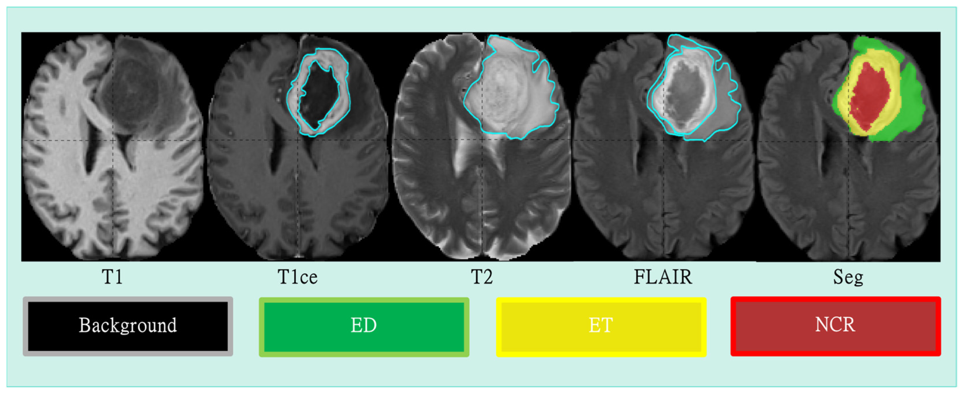
Figure 1. Four MRI modalities and brain tumor segmentation images.
Electronics 14 01658 g001
Figure 2. Schematic diagram of brain tumor segmentation architecture.
Electronics 14 01658 g002
Figure 3. An illustration of the proposed GMDNet for brain tumor image segmentation.
Electronics 14 01658 g003
Figure 4. The grouped encoder feature processing workflow. (a) For the schematic diagram of the data flow inside the grouped encoder, (bd) are the internal structure of the BTA Block.
Electronics 14 01658 g004
Figure 5. An illustration of FMA Block.
Electronics 14 01658 g005
Figure 6. An illustration of the MAA block.
Electronics 14 01658 g006
Figure 7. The use of the BraTS training and validation datasets.
Electronics 14 01658 g007
Figure 8. Experimental flowchart.
Electronics 14 01658 g008
Figure 9. Visualization results of medical cases. The union of green, yellow and red, the union of red and yellow, and the yellow labels represent WT, TC, and ET, respectively.
Electronics 14 01658 g009
Figure 10. The Dice (%) results of ablation study of each component in GMDNet.
Electronics 14 01658 g010
Figure 11. Schematic diagram of the GMD architecture experiment. (A) For Encoder-Decoder architecture, (B) For GMD architecture.
Electronics 14 01658 g011
Figure 12. Comparison of Dice (%) results using different segmentation methods in incomplete modality.
Electronics 14 01658 g012
Figure 13. Diagram of single modality segmentation experiment. (A), (B), (C) and (D) represent single modality experiments of T1, T1ce, T2 and FLAIR respectively.
Electronics 14 01658 g013
Figure 14. The effect of reusing modality results. (a) Represents the segmentation result in the absence of T1; (b) denotes the reuse of FLAIR to compensate for absent T1; (c) indicates segmentation under complete modality. Red, yellow, and green represent NCR, ET, and ED areas respectively.
Electronics 14 01658 g014
Figure 15. The effect of reusing modality results. (a) Represents the segmentation result in the absence of T1ce; (b) denotes the reuse of T2 to compensate for absent T1ce; (c) indicates segmentation under complete modality. Red, yellow, and green represent NCR, ET, and ED areas respectively.
Electronics 14 01658 g015
Figure 16. The effect of reusing modality results. (a) Represents the segmentation result in the absence of T2; (b) denotes the reuse of FLAIR to compensate for absent T2; (c) indicates segmentation under complete modality. Red, yellow, and green represent NCR, ET, and ED areas respectively.
Electronics 14 01658 g016
Figure 17. The effect of reusing modality results. (a) Represents the segmentation result in the absence of FLAIR; (b) denotes the reuse of T1 to compensate for absent FLAIR; (c) indicates segmentation under complete modality. Red, yellow, and green represent NCR, ET, and ED areas respectively.
Electronics 14 01658 g017
Figure 18. Missing, Reuse, and Complete Modality results for each modality. (a) Missing T1 and Reuse of FLAIR; (b) Missing T1ce and Reuse of T2; (c) Missing T2 and Reuse of FLAIR; (d) Missing FLAIR and Reuse of T1.
Electronics 14 01658 g018
Table 1. Model parameter configuration.
Basic ConfigurationValue
PyTorch Version1.10.0
Python3.8.10
GPUNVIDIA GeForce RTX 4090 GPU (24 G)
Cuda11.3
Learning Rate1 × 10−4
OptimizerRanger
Batch Size1
Table 2. Comparison with online results on the BraTS 2018 dataset.
MethodsDice (%)HD 95 (mm)
WTTCETAVGWTTCETAVG
3D U-Net [18]88.5371.7775.9678.7517.1011.626.0411.59
V-Net [61]89.6081.0076.6082.406.547.827.217.19
DMFNet [65]89.9083.5078.1083.834.867.743.385.33
HDCNet [66]88.5084.8076.6083.307.897.097.217.40
TransUNet (2022) [38]89.9582.0478.3883.467.117.674.286.35
mmformer (2022) [67]89.6485.7877.6184.344.438.043.275.25
MVKS-Net (2023) [68]90.0083.3979.8884.423.957.632.314.63
MSFR-Net (2023) [69]90.9085.8080.7085.804.246.722.734.82
RFTNet (2024) [20]90.3082.1580.2484.235.976.413.165.18
SPA-Net (2024) [70]89.6385.8979.9085.144.795.402.774.32
GMDNet (Ours)91.2187.1180.9786.434.435.572.634.21
Table 3. Comparison with online results on the BraTS 2021 dataset.
MethodsDice (%)HD 95 (mm)
WTTCETAVGWTTCETAVG
3D U-Net [18]88.0276.1776.2080.139.9721.5725.4819.01
Att-Unet [71]89.7481.5979.6083.648.0914.6819.3714.05
UNETR [72]90.8983.7380.9385.184.7113.3821.3913.16
TransBTS [38]90.4583.4981.1785.036.7710.1418.9411.95
VT-UNet [73]91.6684.4180.7585.614.1113.2015.0810.80
AABTS-Net (2022) [74]92.2086.1083.0087.104.0011.1817.7310.97
E1D3 UNet (2022) [19]92.4086.5082.2087.034.239.6119.7311.25
Swin Unet3D (2023) [39]90.5086.6083.4086.83----
SDS-Net (2023) [75]91.8086.8082.5087.0321.0711.9913.1315.40
QT-UNet-B (2024) [76]91.2483.2079.9984.814.4412.9517.1911.53
Yaru3DFPN (2024) [77]92.0286.2780.9086.404.098.4321.9111.48
GMDNet (Ours)91.8787.2583.1687.425.168.2218.2710.55
Table 4. Ratio (in %) of the improvement in the performance of GMDNet compared to different methods. Bold numbers indicate statistical significance (p < 0.05).
MethodsWTTCET
%Subjectsp%Subjectsp%Subjectsp
GMDNet vs. 3D U-Net79.281.20 × 10−884.061.35 × 10−780.080.00129
GMDNet vs. Att-Unet78.493.04 × 10−683.271.75 × 10−680.080.00419
GMDNet vs. TransBTS84.061.75 × 10−685.262.60 × 10−783.271.83 × 10−6
GMDNet vs. UNETR78.091.47 × 10−585.661.51 × 10−980.080.00187
GMDNet vs. SwinUnet3D71.310.0072481.270.0002978.490.00296
Table 5. The results of ablation study of each component in GMDNet.
Experiment.BTAFMAMAADPDice (%)
WTTCETAvg
A (w/o Group) 89.5581.6676.2282.47
B 91.6584.7076.1484.16
C 91.8086.1782.6686.87
D 91.2485.1882.9186.44
E 89.9185.0881.3685.45
F 91.9586.3182.9087.05
G (GMDNet)91.8787.2583.1687.42
Table 6. The results of the GMD architecture experiment.
ExperimentFLOPsParameterDice (%)
WTTCETAvg
A746.371 G48.128 M89.9185.9282.4186.08
B (GMDNet)989.921 G35.416 M91.8787.2583.1687.42
Table 7. Comparison with different segmentation networks in incomplete modality.
T1T1ceT2FLAIRMethodsDice (%)
WTTCETAvg
OHeMIS85.772.966.274.93
U-HVED88.277.571.779.13
RobustSeg88.280.368.679.03
mmformer88.1479.5575.6781.12
IMS2 Trans(2024)89.4781.4776.1982.37
GMDNet (Ours)90.7686.1279.7785.55
OHeMIS85.958.032.958.93
U-HVED87.462.133.460.96
RobustSeg87.665.635.662.93
mmformer87.7571.5247.7068.99
IMS2 Trans(2024)88.7771.7042.5967.68
GMDNet (Ours)90.6775.1654.0773.3
OHeMIS83.071.166.373.46
U-HVED86.377.169.977.76
RobustSeg87.777.970.678.73
mmformer87.3379.8075.4780.86
IMS2 Trans(2024)89.0282.5576.0382.53
GMDNet (Ours)89.6186.2080.1485.31
OHeMIS81.272.668.274
U-HVED82.977.872.577.73
RobustSeg85.980.169.478.46
mmformer82.7180.3974.7579.28
IMS2 Trans(2024)88.4482.4276.1682.34
GMDNet (Ours)86.4681.9580.2282.87
Table 8. Experimental results of GMD architecture with single modality.
ModalityDice (%)
WTTCETAvg
T180.6567.4147.8965.31
T1ce80.1978.5379.4779.39
T287.9372.0754.0371.34
FLAIR91.0470.7048.9370.22
Table 9. MRI modalities and tumor regions correlation reference.
ModalityWTTCET
T1LowLowLow
T1ceLowHighHigh
T2HighMediumLow
FLAIRHighLowLow
Table 10. The reuse modality results of missing T1.
Reuse Modality→Missing ModalityDice (%)
WTTCETAvg
Missing T191.8386.2881.386.47
T1ce→T191.9286.6180.786.41
T2→T191.8885.2880.7185.95
FLAIR→T192.0186.3183.287.17
Table 11. The reuse modality results of missing T1ce.
Reuse Modality→Missing ModalityDice (%)
WTTCETAvg
Missing T1ce90.4675.254.2373.29
T1→T1ce91.5175.6756.8674.68
T2→T1ce91.4876.3257.4275.07
FLAIR→T1ce91.2574.1855.5773.66
Table 12. The reuse modality results of missing T2.
Reuse Modality→Missing ModalityDice (%)
WTTCETAvg
Missing T291.5585.8382.0086.46
T1→T291.6685.6483.1186.80
T1ce→T291.3485.7282.9786.67
FLAIR→T291.7186.4982.5386.91
Table 13. The reuse modality results of missing FLAIR.
Reuse Modality→Missing ModalityDice (%)
WTTCETAvg
Missing FLAIR86.6581.3879.5982.54
T1→FLAIR89.5386.3682.7886.22
T2→FLAIR89.4786.5381.8985.96
T1ce→FLAIR89.3685.6682.8985.97
Disclaimer/Publisher’s Note: The statements, opinions and data contained in all publications are solely those of the individual author(s) and contributor(s) and not of MDPI and/or the editor(s). MDPI and/or the editor(s) disclaim responsibility for any injury to people or property resulting from any ideas, methods, instructions or products referred to in the content.