Microwave Imaging of Uniaxial Objects Using a Hybrid Input U-Net

Abstract

This paper introduces hybrid inputs using Internet of Things (IoT) sensors for reconstructing microwave images of uniaxial objects. Specifically, scattered field data is obtained through IoT sensors, and artificial intelligence techniques are employed to enable real-time electromagnetic imaging. The presented method combines a U-Net architecture with an integrated input to reconstruct high-resolution images of dielectric targets for both Transverse Magnetic (TM) and Transverse Electric (TE) waves. The z-axial dielectric constants are reconstructed by the TM wave illumination, while the x- and y-axial dielectric constants are recovered by the TE wave illumination. First, a Direct Sampling Method (DSM) gives spatial details of the target. Second, a Back-propagation (BP) scheme provides basic information about the target’s properties. Lastly, we combine these two inputs by taking their product, which is further processed in the U-Net. Numerical results show that this integration can improve image quality with nearly no additional computing burden. Experiments also reveal that our proposed method is both accurate and efficient for uniaxial objects, making it a reliable solution to overcome the challenges in electromagnetic imaging.

1. Introduction

Electro-Magnetic Imaging (EMI) and the Internet of Things (IoT) are converging to enhance sensing, monitoring, and automation. IoT-enabled EMI systems facilitate real-time data collection, wireless transmission, and cloud-based analysis for applications like structural health monitoring, biomedical imaging, security, environmental sensing, and autonomous systems. This integration enhances efficiency, enables predictive maintenance, and supports smarter decision-making across industries. Electromagnetic imaging is a critical technology in modern science and engineering, with extensive applications in medical imaging, Non-Destructive Testing (NDT), body scanning, object detection, environmental assessment, and disaster rescue. As technology continues to advance, the demand for electromagnetic imaging has grown significantly, requiring not only improvements in imaging accuracy and resolution but also enhancements in computational speed to achieve real-time imaging and meet the requirements for higher-quality imaging.

Recently, the application of neural networks has become a significant trend in the field of image reconstruction. As a result, common image reconstruction methods can be categorized into traditional optimization algorithms and neural network-based optimization algorithms. Traditional optimization algorithms are typically grounded in physical models and mathematical formulas, offering advantages in theoretical stability and interpretability. These methods excel at accurately describing scattering phenomena or the characteristics of physical fields, making them particularly suitable for low-noise environments or scenarios with known target models. In 2020, Kang proposed single- and multi-frequency Direct Sampling Methods (DSMs) for limited-aperture inverse scattering problems. The study introduced a mathematical analysis of DSMs, improving imaging performance by designing multi-frequency indicator functions to enhance robustness and accuracy. Numerical simulations with synthetic and experimental data demonstrated the effectiveness of these methods [1]. In 2021, Harris proposed three DSMs for inverse scattering problems based on the factorization method. The study introduced indicator functions with Tikhonov regularization and conducted rigorous resolution analysis. Numerical simulations demonstrated their effectiveness in reconstructing scatterer shapes with high stability [2]. In 2022, Mahdinezhad proposed hybrid microwave imaging approaches that combine Time-Domain (TD) and Frequency-Domain (FD) algorithms. These methods integrate FD-based prior information to enhance TD convergence and use early TD iterations to improve FD accuracy. Experimental and synthetic results demonstrated that these hybrid techniques significantly reduce computation time while improving imaging resolution and accuracy [3]. In 2023, Yu proposed a novel inversion strategy for solving inverse scattering problems with inhomogeneous media. This method, termed the Multiscaling Differential Contraction Integral Equation (MS-DCIE), integrates the multiscaling regularization scheme with the differential contraction integral equation formulation. By mitigating nonlinearity and ill-posedness, the MS-DCIE achieves high-resolution reconstructions without the need to compute Green’s functions of inhomogeneous backgrounds. Numerical and experimental results highlight its efficiency and robustness, demonstrating superior performance compared to traditional state-of-the-art approaches, particularly in reducing computational costs and improving reconstruction accuracy [4]. In 2024, Li proposed a hybrid solver combining the spectral-integral method and the spectral element method for electromagnetic scattering and inverse scattering problems involving anisotropic objects under TE polarization. Numerical experiments demonstrated the solver’s accuracy and its capability to reconstruct multiple anisotropic parameters [5].

However, traditional methods may face limitations in computational efficiency and convergence speed when dealing with high-dimensional data or nonlinear problems. In contrast, neural network-based optimization algorithms leverage the nonlinear fitting capabilities and powerful data-driven characteristics of deep learning, enabling efficient handling of high-dimensional data in complex scenarios and achieving fast and accurate reconstruction. Furthermore, neural networks can accelerate inference through pretrained models, making them especially advantageous for real-time imaging demands. In 2019, Li proposed a deep Convolutional Neural Network (CNN) designed for electromagnetic inverse scattering problems. The study established a connection between CNN architecture and iterative solution methods, demonstrating that this method provides superior image quality and computational efficiency compared to conventional techniques [6]. In 2020, Yao proposed an enhanced deep learning approach based on a complex-valued deep convolutional encoder–decoder architecture for solving electromagnetic inverse scattering problems. The proposed model directly reconstructs high-contrast scatterers’ permittivity from scattered field data. Numerical benchmarks demonstrated its ability in challenging scenarios involving high-contrast targets [7]. Same year, Lu and collaborators proposed a learning-based quantitative microwave imaging framework utilizing a hybrid input scheme. This framework combines the DSM and BP with a CNN to enhance the reconstruction quality of high-resolution dielectric targets. The hybrid input scheme, which integrates spatial information from DSM and preliminary parameters from BP, significantly improves the performance of U-net CNN without additional computational costs. Numerical and experimental results demonstrate its ability to achieve high-accuracy imaging while maintaining computational efficiency, providing a real-time solution for microwave imaging problems [8]. In 2021, Li proposed a multifrequency U-Net CNN for solving electromagnetic inverse scattering problems. The method leverages multifrequency BP results to train the CNN, significantly improving the accuracy and stability of inversion results for high-contrast scatterers [9]. In 2022, Xu proposed a Scalable Cascaded Convolutional Neural Network (SC-CNN) to incorporate multiresolution labels for the reconstruction. Numerical results demonstrated that SC-CNN achieves superior inversion accuracy and computational efficiency compared to conventional BP-U-Net and direct inversion schemes [10]. That same year, Han proposed a hybrid microwave imaging method combining the Linear Sampling Method (LSM), Born Iterative Method (BIM), and a CNN U-Net for 3-D object reconstruction. This method leverages LSM for initial shape estimation, refines results with the U-Net, and applies BIM in a reduced domain to retrieve dielectric properties. Numerical results demonstrated its ability to achieve higher accuracy and lower computational cost compared to standalone BIM [11]. In 2023, Liu proposed an intelligent electromagnetic inverse scattering framework that combines deep learning techniques and information metasurfaces. The study introduced the Contrast Source Inversion Generative Adversarial Network (CSI-GAN), a physics-informed unsupervised learning method that integrates contrast source inversion (CSI) with a generative adversarial network (GAN). Numerical simulations demonstrated its ability to achieve high-resolution imaging with reduced data acquisition and computational costs [12]. In 2024, Yao proposed a novel deep learning framework for Electro-Magnetic Inverse Scattering Problems (EMIS) using a Conditional Generative Adversarial Network (CDCGAN). The CDCGAN-EMIS integrates a generator, discriminator, and forward solver to establish a mapping between scattered electromagnetic fields and high-contrast permittivity distributions. Numerical experiments demonstrated its ability to handle highly nonlinear and high-contrast scenarios with superior accuracy [13]. The key contributions of this paper are as follows:

• To the best of our knowledge, there is no prior research that integrates BP and DSM as hybrid input measures within the U-Net architecture for uniaxial object imaging. The proposed method effectively leverages BP’s capability to reconstruct dielectric properties and DSM’s ability to extract spatial information, significantly improving reconstruction accuracy while maintaining minimal computational cost.
• This paper tackles the nonlinear effects and field coupling challenges in TE wave-based imaging, which are inherently more complex than in TM waves. By refining the hybrid inputs and incorporating precise incident angle adjustments, the proposed method can effectively mitigate the aforementioned issues, resulting in more stable and accurate reconstructions.
• Extensive numerical simulations demonstrate that the BP-DSM hybrid input mechanism achieves higher accuracy and an improved Structural Similarity Index Measure (SSIM) compared to the use of the BP scheme alone. Moreover, the proposed method also exhibits strong performance even under high noise conditions (e.g., 20% Gaussian noise), showcasing its robustness and applicability to real-world electromagnetic environments.

Section 2 introduces the theoretical basis of electromagnetic wave propagation and inverse scattering problems. Section 3 introduces the U-Net architecture. Section 4 provides numerical simulation results. Section 5 gives the conclusion of this paper.

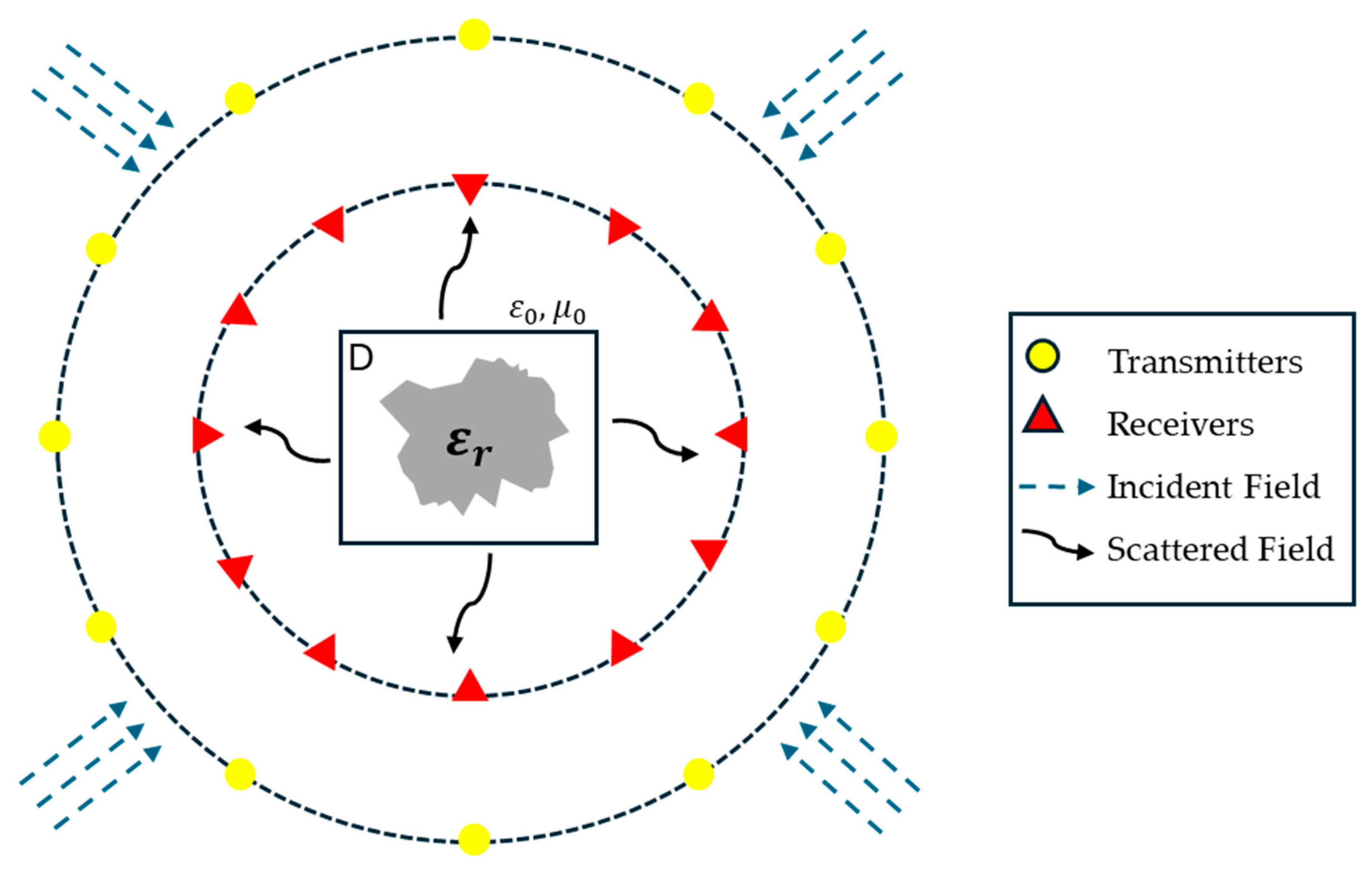
2. Formulation of the Problem

2.1. Direct Problem

Figure 1 illustrates a typical microwave imaging setup for inverse scattering problems. The diagram consists of transmitters (yellow circles) and receivers (red triangles) arranged in a circular configuration around an unknown dielectric target, represented by ${\epsilon }_r$ inside the domain $D$. Transmitters emit electromagnetic waves (yellow curved arrows) toward the imaging region. These waves interact with the unknown object inside $D$, which has a relative permittivity ${\epsilon }_r$ and is surrounded by a free-space medium with permittivity ${\epsilon }_0$ and permeability ${\mu }_0$. As the waves scatter upon encountering the target, receivers capture the scattered field (red arrows), which contains crucial information about the object’s shape, location, and material properties. The collected scattered field data is then used in an inverse reconstruction algorithm, such as BP or the DSM, to estimate the dielectric distribution of the target.

The direct scatter problem can be considered as two separate incident fields. One is the TM wave propagating along the z-axis ($E_z^i$) and the other is the TE wave ($E_x^i$ and $E_y^i$). The scattered field can be obtained by using the Hankel function (Green’s function in two-dimensional cases) [14]. For numerical calculations of the direct problem, we can apply the moment method to transform the integral equations into matrix forms as follows:

$$-\left(E_z^i\right)=\left(\left[G_1\right]\left[{\tau }_z\right]-\left[I\right]\right)\left(E_z\right)$$

(1)

$$\left(E_z^s\right)=\left[G_2\right]\left[{\tau }_z\right]\left(E_z\right)$$

(2)

$$\left(\begin{array}{c}{-E}_x^i\\ {-E}_y^i\end{array}\right)=\left\{\left[\begin{array}{cc}\left[G_3\right]& \left[G_4\right]\\ \left[G_4\right]& \left[G_5\right]\end{array}\right]\left[\begin{array}{cc}\left[{\tau }_x\right]& 0\\ 0& \left[{\tau }_y\right]\end{array}\right]-\left[\begin{array}{cc}\left[I\right]& 0\\ 0& \left[I\right]\end{array}\right]\right\}\left(\begin{array}{c}{E}_x\\ E_y\end{array}\right)$$

(3)

$$\left(\begin{array}{c}{E}_x^s\\ E_y^s\end{array}\right)=\left\{\left[\begin{array}{cc}\left[G_6\right]& \left[G_7\right]\\ \left[G_7\right]& \left[G_8\right]\end{array}\right]\left[\begin{array}{cc}\left[{\tau }_x\right]& 0\\ 0& \left[{\tau }_y\right]\end{array}\right]\right\}\left(\begin{array}{c}{E}_x\\ E_y\end{array}\right)$$

(4)

The Green’s function matrix can be expressed as:

$${\left(G_1\right)}_{mn}=\left\{\begin{array}{c}-{\displaystyle \frac{j\pi k_0{a}_n}{2}}{J}_1\left(k_0{a}_n\right){H_0}^{\left(2\right)}\left(k_0{\rho }_{mn}\right), m\ne n\hfill \\ -{\displaystyle \frac{j}{2}}\left[{\pi k}_0{a}_n{H_1}^{\left(2\right)}\left(k_0{a}_n\right)-2j\right] , m=n\hfill \end{array}\right.$$

(5)

$${\left(G_2\right)}_{mn}=-{\displaystyle \frac{j\pi k_0{a}_n}{2}}{J}_1\left(k_0{a}_n\right){H_0}^{\left(2\right)}\left(k_0{\rho }_{mn}\right)$$

(6)

$$\left(G_3\right)=\left\{\begin{array}{c}-{\displaystyle \frac{j\pi a_n{J}_1\left(k_0{a}_n\right)}{2{{\rho }^3}_{mn}}}\times \left[k{\rho }_{mn}{\left(y_m-y_n\right)}^2{H_0}^{\left(2\right)}\left(k_0{\rho }_{mn}\right)\right.+\\ \begin{array}{cc}\left.({\left(x_m-x_n\right)}^2-{(y_m-y_n)}^2){H_1}^{\left(2\right)}\left(k_0{\rho }_{mn}\right)\right]& , m\ne n \end{array}\\ -{\displaystyle \frac{j}{4}}\left[\pi k_0{a}_n{H_1}^{\left(2\right)}\left(k_0{a}_n\right)-4j\right] , m=n\end{array}\right\}$$

(7)

$$\left(G_4\right)=\left\{\begin{array}{c}-{\displaystyle \frac{j\pi a_n{J}_1\left(k_0{a}_n\right)}{2{{\rho }^3}_{mn}}}\left(x_m-x_n\right)\left(y_m-y_n\right)\times \\ \begin{array}{cc}\left[2{H_1}^{\left(2\right)}\left(k_0{\rho }_{mn}\right)-k_0{\rho }_{mn}{H_0}^{\left(2\right)}\left(k_0{\rho }_{mn}\right)\right]& , m\ne n \end{array}\\ 0 , m=n\end{array}\right\}$$

(8)

$$\left(G_5\right)=\left\{\begin{array}{c}-{\displaystyle \frac{j\pi a_n{J}_1\left(k_0{a}_n\right)}{2{{\rho }^3}_{mn}}}\times \left[k_0{\rho }_{mn}{\left(x_m-x_n\right)}^2{H_0}^{\left(2\right)}\left(k_0{\rho }_{mn}\right)+\right.\\ \begin{array}{cc}\left.({(y_m-y_n)}^2-{\left(x_m-x_n\right)}^2)\right]& , m\ne n \end{array}\\ -{\displaystyle \frac{j}{4}}\left[\pi k_0{a}_n{H_1}^{\left(2\right)}\left(k_0{a}_n\right)-4j\right] , m=n\end{array}\right\}$$

(9)

$$\left(G_6\right)=-{\displaystyle \frac{j\pi a_n{J}_1\left(k_0{a}_n\right)}{2{{\rho }^3}_{mn}}}\times \left[k_0{\rho }_{mn}{\left(y_m-y_n\right)}^2{H_0}^{\left(2\right)}\left(k_0{\rho }_{mn}\right)+({\left(x_m-x_n\right)}^2-{(y_m-y_n)}^2){H_1}^{\left(2\right)}\left(k_0{\rho }_{mn}\right)\right]$$

(10)

$${\left(G_7\right)}_{mn}=-{\displaystyle \frac{j\pi a_n{J}_1\left(k_0{a}_n\right)}{2{{\rho }^3}_{mn}}}\left(x_m-x_n\right)(y_m-y_n)\left[2{H_1}^{\left(2\right)}\left(k_0{\rho }_{mn}\right)-k_0{\rho }_{mn}{H_0}^{\left(2\right)}\left(k_0{\rho }_{mn}\right)\right]$$

(11)

$${\left(G_8\right)}_{mn}=-{\displaystyle \frac{j\pi a_n{J}_1\left(k_0{a}_n\right)}{2{{\rho }^3}_{mn}}}\left[k_0{\rho }_{mn}{\left(x_m-x_n\right)}^2{H_0}^{\left(2\right)}\left(k_0{\rho }_{mn}\right)+({(y_m-y_n)}^2-{\left(x_m-x_n\right)}^2){H_1}^{\left(2\right)}\left(k_0{\rho }_{mn}\right)\right]$$

(12)

Here, ${\rho }_{mn}$ is defined as the distance between the $m-th$ observation point ($x_m, y_m$) and the $n-th$ source point ($x_m, y_m$), given by ${\rho }_{mn}=\sqrt{{\left(x_m-x_n\right)}^2+{\left(y_m-y_n\right)}^2}$. The function $H_0^{\left(2\right)}$ represents the zero-order Hankel function of the second kind, $H_1^{\left(2\right)}$ is the first-order Hankel function of the second kind, and $J_1$ denotes the first-order Bessel function. The column vectors $\left(E_x\right)$, $(E_y)$ and $\left(E_z\right)$ consist of $N$ elements that represent the total field, while the corresponding incident field vectors ${(E}_x^i)$, ${(E}_y^i)$ and ${(E}_z^i)$ also have N-element. In contrast, the scattered field is represented by the column vectors $\left(E_x^s\right)$, $(E_y^s),$ and $\left(E_z^s\right)$, which each contain $M$ elements, where $M$ is the number of measurement points. Moreover, the matrices $\left[{\mathrm{G}}_1\right]$, $\left[{\mathrm{G}}_3\right]$, $\left[{\mathrm{G}}_4\right]$ and $\left[{\mathrm{G}}_5\right]$ are $N\times N$ square matrices, while $\left[{\mathrm{G}}_2\right]$, $\left[{\mathrm{G}}_6\right]$, $\left[{\mathrm{G}}_7\right]$ and $\left[{\mathrm{G}}_8\right]$ are M $\times$ N matrices. The diagonal matrices ${\left({\tau }_x\right)}_{nn}={\epsilon }_x\left(\overline{r}\right)-1$, ${\left({\tau }_y\right)}_{nn}={\epsilon }_y\left(\overline{r}\right)-1$ and ${\left({\tau }_z\right)}_{nn}={\epsilon }_z\left(\overline{r}\right)-1$, respectively, are $N\times N$ matrix. Additionally, $\left[I\right]$ denotes the $N\times N$ identity matrix.

2.2. Back-Propagation (BP)

In scattering problems, the scattered field is recorded outside the scatterer. In the TM case, the dielectric constant ${\epsilon }_z$ is the only unknown parameter. Whereas, in the TE case, both ${\epsilon }_x$ and ${\epsilon }_y$ are the unknown variables. As a result, the reconstruction process would involve determining ${\epsilon }_z$ for TM polarization and ${\epsilon }_x$,${\epsilon }_y$ for TE polarization. To achieve this, BP and DSM are applied to obtain an initial approximation of the dielectric constant distribution tensor. Finally, a U-Net-based deep learning framework is employed to refine these estimates, leading to a more precise reconstruction.

In this part, the measured scattered field is used to obtain an initial estimation of the permittivity distribution through BP, helping to streamline the U-Net training process. Our findings suggest that BP can efficiently approximate the dielectric constants for weak scatterers. The induced currents $I_z^b, I_x^b$, and $I_y^b$ are assumed to be directly proportional to the BP waves as follows:

$$\left(I_z^b\right)={\xi }_m·{\left[G_2\right]}^H\left(E_z^s\right)$$

(13)

$$\left(\begin{array}{c}{I}_x^b\\ I_y^b\end{array}\right)={\xi }_e·{\left[\begin{array}{cc}\left[G_6\right]& \left[G_7\right]\\ \left[G_7\right]& \left[G_8\right]\end{array}\right]}^H\left(\begin{array}{c}{E}_x^s\\ E_y^s\end{array}\right)$$

(14)

where H represents the Hermitian (conjugate transpose) operation. To minimize the difference between the measured field and the calculated field from the $I_z^b, I_x^b$, and $I_y^b$ obtained in Equations (13) and (14), the values ${\xi }_m$ and ${\xi }_e$ are derived as follows:

$${\xi }_m={\displaystyle \frac{{\left(E_z^s\right)}^T·{\left(\left[G_2\right]\left({\left[G_2\right]}^H·\left(E_z^s\right)\right)\right)}^{*}}{{‖\left[G_2\right]\left({\left[G_2\right]}^H·\left(E_z^s\right)\right)‖}^2}}$$

(15)

$${\xi }_e={\displaystyle \frac{{\left(\begin{array}{c}{E}_x^s\\ E_y^s\end{array}\right)}^T·{\left(\left[\begin{array}{cc}\left[G_6\right]& \left[G_7\right]\\ \left[G_7\right]& \left[G_8\right]\end{array}\right]\left({\left[\begin{array}{cc}\left[G_6\right]& \left[G_7\right]\\ \left[G_7\right]& \left[G_8\right]\end{array}\right]}^H·\left(\begin{array}{c}{E}_x^s\\ E_y^s\end{array}\right)\right)\right)}^{*}}{{‖\left[\begin{array}{cc}\left[G_6\right]& \left[G_7\right]\\ \left[G_7\right]& \left[G_8\right]\end{array}\right]\left({\left[\begin{array}{cc}\left[G_6\right]& \left[G_7\right]\\ \left[G_7\right]& \left[G_8\right]\end{array}\right]}^H·\left(\begin{array}{c}{E}_x^s\\ E_y^s\end{array}\right)\right)‖}^2}}$$

(16)

where $T$ represents the transpose operation, and * denotes the matrix operation of complex conjugate. Once ${\xi }_m$ and ${\xi }_e$ are obtained, the total BP wave $E_z^b$, $E_x^b$, and $E_y^b$ are determined through the BP current by the following equations:

$$\left(E_z^b\right)=\left(E_z^i\right)+\left[G_1\right]\left(I_z^b\right)$$

(17)

$$\left(\begin{array}{c}{E}_x^b\\ E_y^b\end{array}\right)=\left(\begin{array}{c}{E}_x^i\\ E_y^i\end{array}\right)+\left[\begin{array}{cc}\left[G_3\right]& \left[G_4\right]\\ \left[G_4\right]& \left[G_5\right]\end{array}\right]\left(\begin{array}{c}{I}_x^b\\ I_y^b\end{array}\right)$$

(18)

The contrasts $\left[{\tau }_z^b\right], \left[{\tau }_x^b\right] \mathrm{and} \left[{\tau }_y^b\right]$ are linearly proportional to the BP currents and can be expressed as:

$$\left(I_{z,p}^b\right)=diag\left(\left[{\tau }_z^b\right]\right)\left(E_z^b\right)$$

(19)

$$\left(\begin{array}{c}{I}_{x,p}^b\\ I_{y,p}^b\end{array}\right)=diag\left(\left[\begin{array}{cc}\left[{\tau }_x^b\right]& 0\\ 0& \left[{\tau }_y^b\right]\end{array}\right]\right)\left(\begin{array}{c}{E}_x^b\\ E_y^b\end{array}\right)$$

(20)

By applying the least squares method to all incidences in Equations (19) and (20), the n-th contrasts for $\left[{\tau }_z^b\right], \left[{\tau }_x^b\right] \mathrm{and} \left[{\tau }_y^b\right]$ are determined as follows:

$$\left[{\tau }_z^b\right]={\displaystyle \frac{{\sum }_{p=1}^{N_i}{I}_{z, p}^b\left(n\right)·{\left[E_z^b\left(n\right)\right]}^{*}}{{\sum }_{p=1}^{N_i}{‖E_z^b\left(n\right)‖}^2}}$$

(21)

$$\left[\begin{array}{cc}\left[{\tau }_x^b\right]& 0\\ 0& \left[{\tau }_y^b\right]\end{array}\right]={\displaystyle \frac{{\sum }_{p=1}^{N_i}\begin{array}{c}{I}_{x,p}^b\left(n\right)\\ I_{y,p}^b\left(n\right)\end{array}·{\left[\left(\begin{array}{c}{E}_x^b\\ E_y^b\end{array}\right)\left(n\right)\right]}^{*}}{{\sum }_{p=1}^{N_i}{‖\begin{array}{c}{E}_x^b\left(n\right)\\ E_y^b\left(n\right)\end{array}‖}^2}}$$

(22)

where $N_i$ is the number of incident waves.

2.3. Direct Sampling Methods (DSMs)

The DSM is a simple, fast, and efficient non-iterative sampling technique. Since it only requires input from the scattered field data, it can rapidly reconstruct an initial estimate of the location and size of the target. In this study, for reconstructing surface profiles and conductor shapes, DSM is particularly suitable for retrieving the shape and position of unknown scatterers, as conductors only require shape and size reconstruction. A schematic diagram of this process is shown in Figure 2.

The DSM was initially applied to the two-dimensional dielectric inverse scattering problem with a fixed planar incident wave and was later extended to various inverse scattering problems. DSM is a fast approach as it does not require additional operations such as Singular Value Decomposition (SVD) or solving ill-posed integral equations. The DSM formulation for the TM case is given as follows:

$$\Psi \left(r_p\right)={\displaystyle \frac{1}{N_i}}\sum _{l=1}^{N_i}\hspace{1em}{\displaystyle \frac{\left|⟨{\left(E_z^s\right)}_l\left(r\right),G_2\left(r,r_p\right)⟩\right|}{‖{\left(E_z^s\right)}_l\left(r\right)‖‖G_2\left(r,r_p\right)‖}}$$

(23)

Here, $r_p$ represents the sampling point, while $r$ denotes the position vector of the receiver. $N_r$ is the number of receiving points. The vector ${\left(E_z^s\right)}_l\left(r\right)$, with dimensions $N_r\times 1$, represents the measured scattered field. The term $\left[{\mathrm{G}}_2\right]$ is also an $N_r\times 1$ vector, representing the Green’s function for an excitation source located at $r_p$ and an observation point at $r$. The indicator function in the X-direction is given as follows:

$${\Psi }_x={\displaystyle \frac{1}{N_i}}\sum _{l=1}^{N_i}{\displaystyle \frac{\left|\left(\begin{array}{c}{\left(E_x^s\right)}_l\\ {\left(E_y^s\right)}_l\end{array}\right)·\left(\begin{array}{c}{G}_6\\ G_7\end{array}\right)\right|}{‖\left(\begin{array}{c}{\left(E_x^s\right)}_l\\ {\left(E_y^s\right)}_l\end{array}\right)‖‖\left(\begin{array}{c}{G}_6\\ G_7\end{array}\right)‖}}$$

(24)

The indicator function in the Y-direction is given as follows:

$${\Psi }_y={\displaystyle \frac{1}{N_i}}\sum _{l=1}^{N_i}{\displaystyle \frac{\left|\left(\begin{array}{c}{\left(E_x^s\right)}_l\\ {\left(E_y^s\right)}_l\end{array}\right)·\left(\begin{array}{c}{G}_6\\ G_7\end{array}\right)\right|}{‖\left(\begin{array}{c}{\left(E_x^s\right)}_l\\ {\left(E_y^s\right)}_l\end{array}\right)‖‖\left(\begin{array}{c}{G}_6\\ G_7\end{array}\right)‖}}$$

(25)

When we transmit the TE waves for reconstruction, the magnitude of the incident fields $E_x^i$ and $E_y^i$ will be affected by the angle of the incidence. When $E_x^i$ is large, we can use ${\Psi }_x\left(r_p\right)$ to reconstruct the shape. Similarly, when $E_y^i$ is large, we can use ${\Psi }_y\left(r_p\right)$ to reconstruct the shape. There are 32 incident waves in total.

To fulfill the one-to-one relationship with the neural network, a hybrid input scheme, BP-DSM, i.e., the dot product between the result by DSM and the one by BP, is proposed to achieve the quantitative inversion. The results obtained by BP are used for distinguishing scatterers with the same shape but different permittivity, and the spatial information obtained by DSM can also improve the quality of feature map information compared to using BP alone.

3. U-Net

Figure 3 shows the U-Net architecture used in this study. It consists of a contracting network on the left and an expanding network on the right. The contracting network applies repeated $3\times 3$ convolution and batch normalization as well as Rectified Linear Units (ReLU) to extract and refine image features, followed by a $2\times 2$ max pooling layer for down-sampling. The max pooling layer helps prevent overfitting by selecting the maximum value within non-overlapping regions.

In the expanding network, an up-sampling operation is applied to the upper $3\times 3$ convolution layer to restore spatial resolution. The convolution layers extract features using multiple filters, while batch normalization accelerates training and stabilizes gradient updates by reducing sensitivity to parameter variations. ReLU layers introduce nonlinearity, allowing the model to recognize complex patterns and enhance decision-making. Although this process improves model performance during training, its immediate effects may not always be evident. Here, $N_i$ represents the number of input channels, and $N_{out}$ represents the number of output channels. In this study, $N_i$ is equal to $N_{out}$. In the final stage, a convolution layer with $1\times 1$ size consolidates the extracted features to produce predictions. The key reasons for choosing U-Net are its strong generalization capability, skip connections for gradient stability, and an enhanced receptive field and prediction accuracy.

The objective functions (26) for the U-Net are minimized to obtain ${\epsilon }_z$, ${\epsilon }_x$, and ${\epsilon }_y$:

$$\begin{array}{c}argmin\\ B,i\end{array}:\sum _{N=1}^{N_t}f\left(B\left(\begin{array}{c}{\epsilon }_x^{\alpha }\\ {\epsilon }_y^{\alpha }\\ {\epsilon }_z^{\alpha }\end{array}\right), \left(\begin{array}{c}{\epsilon }_x\\ {\epsilon }_y\\ {\epsilon }_z\end{array}\right)\right)+\Omega \left(i\right)$$

(26)

Equation (26) defines a unified loss function that simultaneously minimizes the reconstruction errors of the three dielectric components ${\epsilon }_x,{\epsilon }_y,$ and ${\epsilon }_z$. The function $f(\cdot )$ evaluates the discrepancy between the predicted permittivity values obtained from the U-Net model $B$ and the corresponding ground truth. By integrating all three components into a single loss formulation, the proposed framework ensures consistent and coordinated learning across different polarization directions. The term $\Omega \left(i\right)$ represents a regularization function applied to stabilize the optimization process.

4. Numerical Results

4.1. Simulation Configuration

In our simulation, the scatterer is partitioned into small cells, each with a side length smaller than ${\displaystyle \frac{0.2{\lambda }_0}{\sqrt{{\epsilon }_r}}}$, where ${\lambda }_0$ represents the free-space wavelength and ${\epsilon }_r$ is the highest relative permittivity among the anisotropic objects. The incident wave operates at a frequency of 3 GHz, and the environment features 32 transmitters and receivers. Both TM and TE polarized plane waves are used to illuminate the scatterers, with Gaussian noise added at levels of 5% and 20% to mimic real-world conditions. For the TM polarization, the transmitters and receivers are arranged at uniform 11.25° intervals, resulting in a total of 32 devices each. The dataset is divided, with 80% allocated for training and 20% reserved for testing. For TE wave reconstruction, the magnitudes of the incident fields $E_x^i$ and $E_y^i$ depend on the angle of incidence. To address this, we fixed the incident angles at specific values: 0°, 2.5°, 5°, 7.5°, and 10° (to enhance $E_y^i$); 82.5°, 85°, 87.5°, 90°, 92.5°, 95°, 97.5°, and 100° (to enhance $E_x^i$); 172.5°, 175°, 177.5°, 180°, 182.5°, 185°, 187.5°, and 190° (again for strong $E_y^i$); 262.5°, 265°, 267.5°, 270°, 272.5°, 275°, 277.5°, and 280° (for strong $E_x^i$); and finally, 352.5°, 355°, and 357.5° (for strong $E_y^i$). When $E_x^i$ is dominant, we use the corresponding scattered field $E_x^s$ to reconstruct ${\epsilon }_x$; similarly, when $E_y^s$ is dominant, $E_y^i$ is used to reconstruct ${\epsilon }_y$. In total, 32 incident waves are utilized.

During training, each U-Net functions independently, making GPU parallelization an effective strategy to greatly enhance computational efficiency. For optimization, we utilize Adaptive Moment Estimation (ADAM), a widely used algorithm in deep learning. ADAM integrates the benefits of both Adaptive Gradient Algorithm (AdaGrad) and Root Mean Square Propagation (RMSProp) by estimating the first and second moments of gradients (mean and variance), allowing it to assign adaptive learning rates to individual parameters. This capability enables dynamic learning rate adjustments, making it particularly useful for handling sparse gradients and noisy data. Additionally, ADAM incorporates bias correction, which is especially important in the early stages of training. Due to its reliability and efficiency, it has become a standard optimization method in deep learning. In this study, the learning rate is set between ${10}^{-3}$ and ${10}^{-5}$, with a total of 40 epochs, where the dataset is shuffled at the start of each epoch to improve training performance. The Root Mean Square Error (RMSE), defined in Equation (27), is utilized to assess the accuracy and effectiveness of each solution.

$$RMSE={\displaystyle \frac{1}{M_t}}\sum _{i=1}^{M_t}{‖{\epsilon }_r-{\epsilon }_r^{\alpha }‖}_F/{‖{\epsilon }_r‖}_F$$

(27)

Here, ${\epsilon }_r^{\alpha }$ represents the reconstructed dielectric constant distribution, while ${\epsilon }_r$ denotes the ground truth. $M_t$ refers to the total number of test cases conducted, and $F$ represents the Frobenius norm. The Structural Similarity Index Measure (SSIM) is defined as follows:

$$SSIM={\displaystyle \frac{\left(2{\mu }_{\tilde{y}}{\mu }_y+C_1\right)\left(2{\sigma }_{\tilde{y}y}+C_2\right)}{\left({\mu }_{\tilde{y}}^2+{\mu }_y^2+C_1\right)\left({\sigma }_{\tilde{y}}^2+{\sigma }_y^2+C_2\right)}}$$

(28)

In this context, $\tilde{y}$ represents the reconstructed relative permittivity profile, while y denotes the true relative permittivity profile. The mean of y is denoted as ${\mu }_y$, the variance of $\tilde{y}$ is given by ${\sigma }_{\tilde{y}}^2$, and the covariance between $\tilde{y}$ and y is represented by ${\sigma }_{\tilde{y}y}$. The constants $C_1$ and $C_2$ are introduced to prevent division by zero, where $C_1={\left(K_{1}D\right)}^2$ and $C_2={\left(K_{2}D\right)}^2.$ Here, $K_1=0.01$ and $K_2=0.03$ are hyperparameters, while $D$ denotes the dynamic range of pixel values in the target image y.

For reference, the relative permittivity of free space (air) is considered as 1.0, serving as the baseline in contrast with the dielectric targets. In our experiments, the dielectric constants of the scatterers are categorized into three groups:

(1)

1.2–1.5, representing materials such as Teflon, PTFE, or dry wood;

(2)

1.5–2.0, corresponding to acrylic, plastics, and epoxy resins;

(3)

2.0–2.5, covering low-loss ceramics, glass, and dense polymer composites.

These values reflect commonly used materials in electromagnetic imaging, ensuring the simulations are representative of practical scenarios.

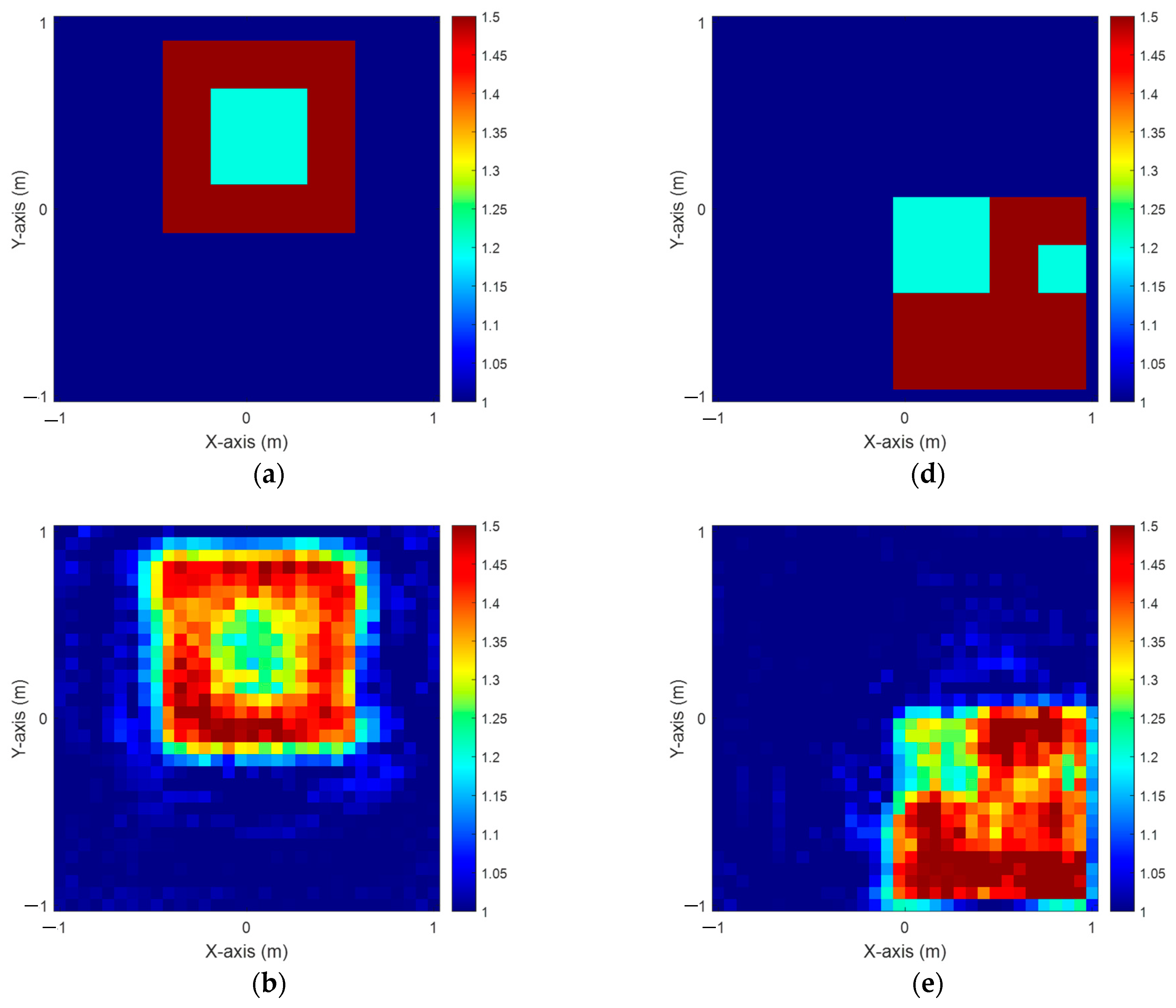
4.2. Dielectric Permittivity Between 1 and 1.5 with 20% Noise

This scenario involves the permittivity distribution ranges between 1 and 1.5 with 20% Gaussian noise. The dataset consists of 500 images from 10 dielectric constant distributions and 50 random locations. We compare the reconstruction results obtained using the pure BP (Back-propagation) scheme and the hybrid BP-DSM scheme with both TM and TE waves. Figure 4a represents the true ${\epsilon }_z$. Figure 4b illustrates the reconstructed ${\epsilon }_z$ by BP. Figure 4c depicts the reconstructed ${\epsilon }_z$ by BP-DSM. Figure 4d represents the true ${\epsilon }_x$. Figure 4e presents the reconstructed ${\epsilon }_x$ by BP. Figure 4f shows the reconstructed ${\epsilon }_x$ by BP-DSM. Comparing either Figure 4b,c or Figure 4e,f clearly demonstrates that the BP-DSM scheme leads to notable improvements in reconstruction quality. The proposed hybrid input method has enhanced the structural details, minimized noise, and achieved a more precise dielectric permittivity distribution compared to using the BP scheme alone.

Table 1. Performance of dielectric constant variation of ${\epsilon }_z$ and ${\epsilon }_x$ from 1 to 1.5 with 20% noise.

Performance	${\mathit{\epsilon }}_{\mathit{z}}$		${\mathit{\epsilon }}_{\mathit{x}}$
	BP	BP-DSM	BP	BP-DSM
RMSE	7.05%	6.38%	5.7%	4.71%
SSIM	81.59%	86.85%	88.17%	92.13%

presents the performance of TM ${\epsilon }_z$ and TE ${\epsilon }_x$ using the BP scheme alone and the hybrid BP-DSM mechanism with 20% Gaussian noise. Numerical results indicate that the hybrid BP-DSM approach outperforms the BP scheme in reconstructing the dielectric constant distribution in high-noise environments and better preserves the structural features of the images.

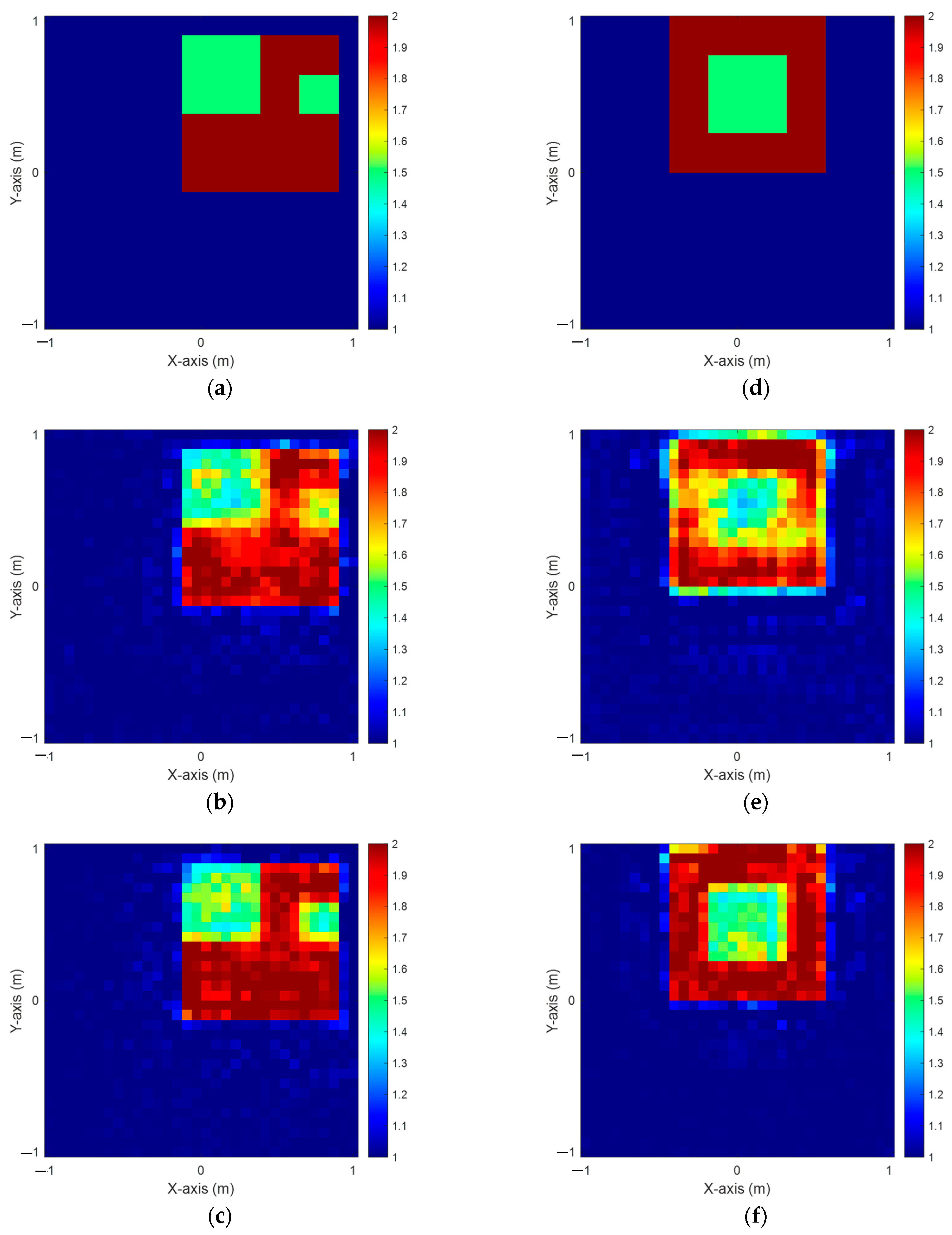
4.3. Dielectric Permittivity Ranges from 1.5 to 2 with 5% Noise

This scenario involves the permittivity distribution ranges between 1.5 and 2 with 5% Gaussian noise. The dataset remains at 500 (10 $\times$ 50) images as in the previous case. The BP and BP-DSM mechanisms are used to reconstruct dielectric objects in both TM and TE wave conditions. Figure 5a represents the true ${\epsilon }_z$. Figure 5b illustrates the reconstructed ${\epsilon }_z$ by the BP scheme. Figure 5c depicts the reconstructed ${\epsilon }_z$ by the hybrid BP-DSM scheme. Figure 5d represents the true ${\epsilon }_x$. Figure 5e presents the reconstructed ${\epsilon }_x$ by the BP scheme. Figure 5f shows the reconstructed ${\epsilon }_x$ by the BP-DSM mechanism. By comparing Figure 5b,c, as well as Figure 5e,f, it is clear that the BP-DSM mechanism markedly improves reconstruction quality and enhances the accuracy of both the object’s shape and its permittivity distribution, outperforming the BP scheme used alone.

From the results in

Table 2. Performance of dielectric constant variation of ${\epsilon }_z$ and ${\epsilon }_x$ between 1.5 and 2 with 5% Gaussian noise.

Performance	${\mathit{\epsilon }}_{\mathit{z}}$		${\mathit{\epsilon }}_{\mathit{x}}$
	BP	BP-DSM	BP	BP-DSM
RMSE	5.7%	4.77%	6.54%	4.51%
SSIM	93.79%	94.03%	93.57%	97.24%

, we observe that the hybrid BP-DSM approach also overwhelms the standalone BP method in reconstructing the distributions of high-contrast dielectric constants in the presence of 5% Gaussian noise.

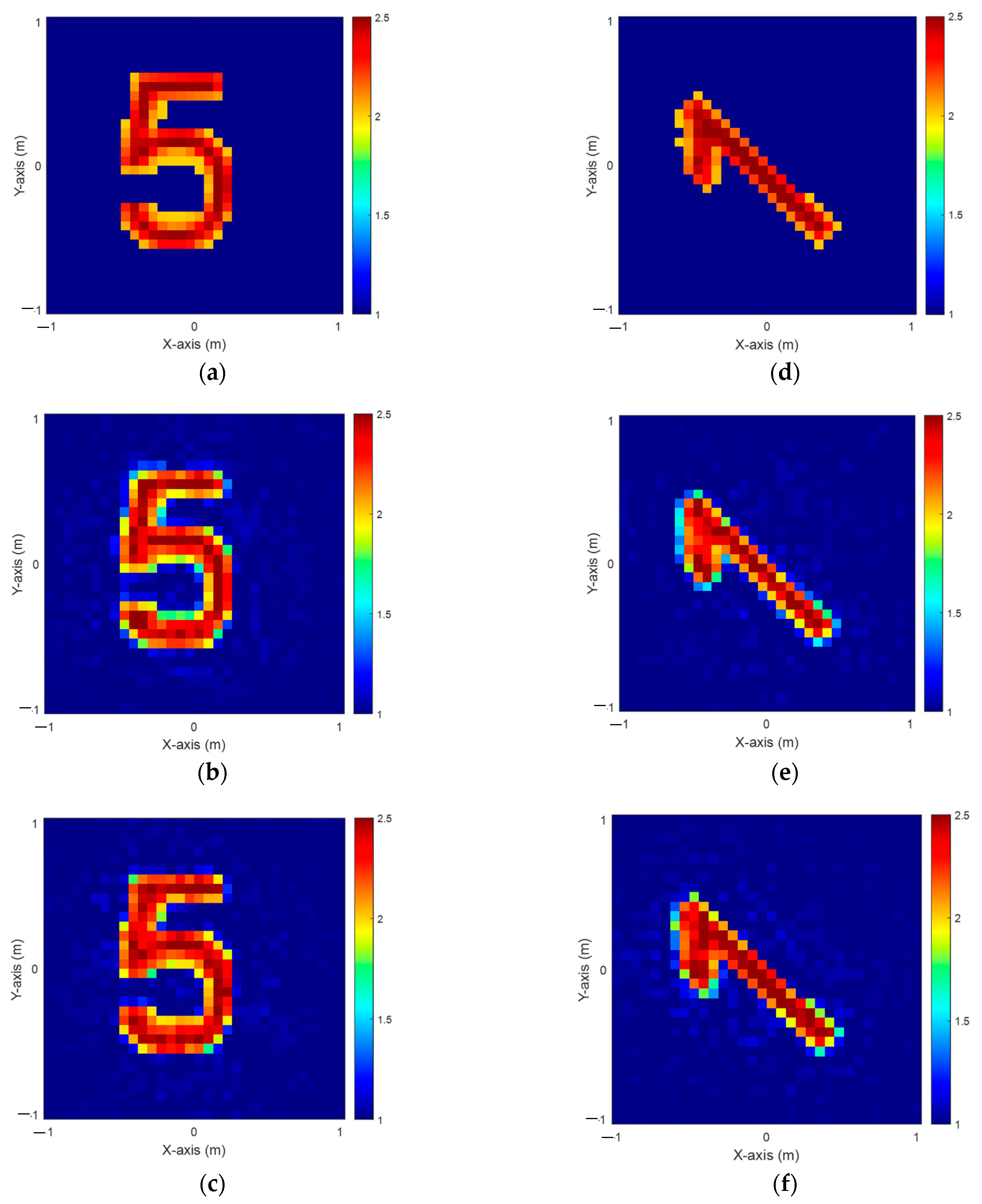
4.4. Dielectric Permittivity Ranges Between 2 and 2.5 with 5% Noise

This scenario further increases the permittivity distribution, which ranges from 2 to 2.5 with 5% Gaussian noise. Reconstruction results for dielectric objects are compared between standalone BP and hybrid BP-DSM in both TM and TE cases. Figure 6a represents the true ${\epsilon }_z$. Figure 6b illustrates the reconstructed ${\epsilon }_z$ by BP. Figure 6c depicts the reconstructed ${\epsilon }_z$ by BP-DSM. Figure 6d represents the true ${\epsilon }_x$. Figure 6e presents the reconstructed ${\epsilon }_x$ by BP. Figure 6f shows the reconstructed ${\epsilon }_x$ by BP-DSM. Similarly, it is apparent from Figure 6b,c, as well as Figure 6e,f, that the BP-DSM hybrid input scheme significantly improves the reconstruction quality by preserving finer structural details, thereby surpassing the BP scheme alone.

Numerical data in

Table 3. Performance of dielectric constant variation of ${\epsilon }_z$ and ${\epsilon }_x$ from 2 to 2.5 with 5% noise.

Performance	${\mathit{\epsilon }}_{\mathit{z}}$		${\mathit{\epsilon }}_{\mathit{x}}$
	BP	BP-DSM	BP	BP-DSM
RMSE	8.37%	7.77%	7.87%	6.51%
SSIM	86.48%	87.1%	86.31%	90.37%

also prove that the BP-DSM mechanism offers superior reconstruction accuracy compared to the standalone BP approach when dealing with the dielectric constant distribution in the presence of 5% Gaussian noise in both TM and TE waves.

To provide a practical sense of computational performance, we report the approximate time consumption for each stage of the proposed method. On a desktop system equipped with an NVIDIA RTX 4060Ti GPU, Intel(R) Core (TM)i7-14700k, and 64 GB RAM. The computation of Green’s function matrices and application of the BP and DSM algorithms takes approximately 3.2 s per image, including data preparation and pre-processing. The training of the U-Net model with 500 samples for 40 epochs requires approximately 1.5 h. Once trained, the inference time per sample is about 0.08 s, enabling real-time reconstruction.

5. Conclusions

In this paper, we propose a novel hybrid input scheme that integrates BP and DSM within a U-Net architecture for microwave imaging of uniaxial objects. By leveraging BP’s strength in reconstructing dielectric properties and DSM’s ability to capture spatial details, our findings underscore the robustness (including noise immunity and reduced computational costs) of the proposed methodology. The hybrid BP-DSM is capable of yielding more reliable and stable permittivity distributions with greater efficiency. Furthermore, by incorporating precise incident angle adjustments, the nonlinear effects and field coupling challenges inherent in the TE wave imaging can be overcome. Additional numerical experiments confirm that this method is able to real-time reconstruct high-permittivity objects, highlighting its tremendous potential for practical applications in electromagnetic inverse scattering problems.

However, when the noise level exceeds 50%, the model begins to lose structural accuracy, especially in preserving object boundaries and background clarity. This indicates a potential limitation of the current approach under extremely noisy conditions. Future work may incorporate denoising strategies or adversarial training to enhance robustness in such scenarios.

References

1. Kang, S.; Lambert, M.; Ahn, C.Y.; Ha, T.; Park, W.K. Single- and Multi-Frequency Direct Sampling Methods in a Limited-Aperture Inverse Scattering Problem. IEEE Access 2020, 8, 121637–121649. [Google Scholar] [CrossRef]
2. Harris, I. Direct sampling algorithms based on the factorization method for inverse scattering. In Proceedings of the 2021 IEEE Research and Applications of Photonics in Defense Conference (RAPID), Miramar Beach, FL, USA, 2–4 August 2021. [Google Scholar]
3. Saraskanroud, F.M.; Jeffrey, I. Hybrid Approaches in Microwave Imaging Using Quantitative Time- and Frequency-Domain Algorithms. IEEE Trans. Comput. Imaging 2022, 8, 121–132. [Google Scholar] [CrossRef]
4. Zhong, Y.; Zardi, F.; Salucci, M.; Oliveri, G.; Massa, A. Multiscaling Differential Contraction Integral Method for Inverse Scattering Problems with Inhomogeneous Media. IEEE Trans. Microw. Theory Tech. 2023, 71, 4064–4079. [Google Scholar] [CrossRef]
5. Li, J.; Li, Z.; Guan, Z.; Han, F. 2-D Electromagnetic Scattering and Inverse Scattering from Anisotropic Objects Under TE Illumination Solved by the Hybrid SIM/SEM. IEEE Trans. Antennas Propag. 2024, 72, 3517–3528. [Google Scholar] [CrossRef]
6. Li, L.; Wang, L.G.; Teixeira, F.L. Performance Analysis and Dynamic Evolution of Deep Convolutional Neural Network for Electromagnetic Inverse Scattering. IEEE Antennas Wirel. Propag. Lett. 2019, 18, 2259–2263. [Google Scholar] [CrossRef]
7. Yao, H.M.; Jiang, L.; Sha, W.E.I. Enhanced Deep Learning Approach Based on the Deep Convolutional Encoder–Decoder Architecture for Electromagnetic Inverse Scattering Problems. IEEE Antennas Wirel. Propag. Lett. 2020, 19, 1211–1215. [Google Scholar] [CrossRef]
8. Zhang, L.; Xu, K.; Song, R.; Ye, X.; Wang, G.; Chen, X. Learning-Based Quantitative Microwave Imaging with a Hybrid Input Scheme. IEEE Sens. J. 2020, 20, 15007–15013. [Google Scholar] [CrossRef]
9. Li, H.; Chen, L.; Qiu, J. Convolutional Neural Networks for Multifrequency Electromagnetic Inverse Problems. IEEE Antennas Wirel. Propag. Lett. 2021, 20, 1424–1428. [Google Scholar] [CrossRef]
10. Xu, K.; Zhang, C.; Ye, X.; Song, R. Fast Full-Wave Electromagnetic Inverse Scattering Based on Scalable Cascaded Convolutional Neural Networks. IEEE Trans. Geosci. Remote Sens. 2022, 60, 2001611. [Google Scholar] [CrossRef]
11. Han, F.; Zhong, M.; Fei, J. Hybrid Microwave Imaging of 3-D Objects Using LSM and BIM Aided by a CNN U-Net. IEEE Trans. Geosci. Remote Sens. 2022, 60, 2006809. [Google Scholar] [CrossRef]
12. Liu, C.; Zhang, H.; Li, L.; Cui, T.J. Towards Intelligent Electromagnetic Inverse Scattering Using Deep Learning Techniques and Information Meta-surfaces. IEEE J. Microwaves 2023, 3, 509–522. [Google Scholar] [CrossRef]
13. Yao, H.M.; Jiang, L.; Ng, M. Enhanced Deep Learning Approach Based on the Conditional Generative Adversarial Network for Electromagnetic Inverse Scattering Problems. IEEE Trans. Antennas Propag. 2024, 72, 6133–6138. [Google Scholar] [CrossRef]
14. Chiu, C.C.; Chen, P.H.; Jiang, H. Electromagnetic Imaging of Uniaxial Objects by Artificial Intelligence Technology. IEEE Trans. Geosci. Remote Sens. 2022, 60, 2008414. [Google Scholar] [CrossRef]
Figure 1. Schematic representation of the inverse scattering setup.
Electronics 14 01633 g001
Figure 2. DSM schematic diagram.
Electronics 14 01633 g002
Figure 3. U-Net architecture.
Electronics 14 01633 g003
Figure 4. Relative permittivity between 1 and 1.5. (a) Ground truth for the ε z (b) BP reconstruction outcomes for the ε z . (c) Hybrid input reconstruction outcomes for the ε z . (d) Ground truth for the ε x . (e) BP reconstruction outcomes for the ε x . (f) Hybrid input reconstruction outcomes for the ε x .
Electronics 14 01633 g004aElectronics 14 01633 g004b
Figure 5. Relative permittivity between 1.5 and 2. (a) Ground truth for the ε z (b) BP reconstruction outcomes for the ε z . (c) Hybrid input reconstruction outcomes for the ε z . (d) Ground truth for the ε x . (e) BP reconstruction outcomes for the ε x . (f) Hybrid input reconstruction outcomes for the ε x .
Electronics 14 01633 g005
Figure 6. Relative permittivity between 2 and 2.5. (a) Ground truth for the ε z . (b) BP reconstruction outcomes for the ε z . (c) Hybrid input reconstruction outcomes for the ε z . (d) Ground truth for the ε x . (e) BP reconstruction outcomes for the ε x . (f) Hybrid input reconstruction outcomes for the ε x .
Electronics 14 01633 g006