DIN-SLAM: Neural Radiance Field-Based SLAM with Depth Gradient and Sparse Optical Flow for Dynamic Interference Resistance

Abstract

The neural implicit SLAM system performs excellently in static environments, offering higher-quality rendering and scene reconstruction capabilities compared to traditional dense SLAM. However, in dynamic real-world scenes, these systems often experience tracking drift and mapping errors. To address these problems, we suggest DIN-SLAM, a dynamic scene neural implicit SLAM system based on optical flow and depth gradient verification. DIN-SLAM combines depth gradients, optical flow, and motion consistency to achieve robust filtering of dynamic pixels, while optimizing dynamic feature points through optical flow registration to enhance tracking accuracy. The system also introduces a dynamic scene optimization strategy that utilizes photometric consistency loss, depth gradient loss, motion consistency constraints, and edge matching constraints to improve geometric consistency and reconstruction performance in dynamic environments. To reduce the interference of dynamic objects on scene reconstruction and eliminate artifacts in scene updates, we propose a targeted rendering and ray sampling strategy based on local feature counts, effectively mitigating the impact of dynamic object occlusions on reconstruction. Our method supports multiple sensor inputs, including pure RGB and RGB-D. The experimental results demonstrate that our approach consistently outperforms state-of-the-art baseline methods, achieving an 83.4% improvement in Absolute Trajectory Error Root Mean Square Error (ATE RMSE), a 91.7% enhancement in Peak Signal-to-Noise Ratio (PSNR), and the elimination of artifacts caused by dynamic interference. These enhancements significantly boost the performance of tracking and mapping in dynamic scenes.

1. Introduction

In recent years, NeRF (neural radiance field) has achieved remarkable results in the field of novel view synthesis, demonstrating extensive application potential in areas such as augmented reality (AR), virtual reality (VR), and scene reconstruction. As one of the core research topics in robotics, SLAM (Simultaneous Localization and Mapping) is regarded as a key technology for solving embodied intelligence and real-time environmental perception problems. SLAM provides foundational support for robots and other autonomous systems by incrementally modeling the environment and estimating positions accurately. In recent years, with the continuous improvement of NeRF performance, combining NeRF with SLAM technology has significantly enhanced SLAM systems’ ability in high-fidelity dense scene reconstruction and greatly expanded NeRF’s application in real-world scenarios, such as dynamic scene reconstruction and real-time perception [1,2].

However, existing neural implicit SLAM systems exhibit strong performance in environments that are static, but still face many challenges in dynamic environments, especially in practical application scenarios such as robotics, drones, or autonomous vehicles [3]. The appearance of dynamic objects introduces significant interference, such as inaccurate depth information and abnormal distribution of dynamic pixels. This interference can lead to error accumulation during tracking and introduce artifacts in scene reconstruction. Furthermore, the real-time processing requirements for large-scale scenes pose higher demands on neural implicit SLAM systems. However, existing systems often lack precise loop closure and global bundle adjustment in dynamic environments, making them susceptible to drift, which significantly degrades the quality of scene mapping [4,5].

To address these issues, recent research has focused on improving dynamic scene modeling methods and optimization strategies to increase the robustness of neural implicit SLAM systems in dynamic environments. These methods include using semantic information and motion features to segment dynamic objects, introducing optical flow or geometric constraints for more precise dynamic pixel filtering, and applying improved global optimization methods to reduce the accumulation of drift [6,7]. Despite some progress, achieving efficient and accurate dynamic scene modeling remains an important research direction in the field of neural implicit SLAM.

Current challenges in NeRF-based SLAM for dynamic scenes primarily include two aspects: (1) Due to the widespread use of frame-to-frame systems based on direct methods, the performance in dynamic scenes is limited. Even with accurate dynamic masks, direct-method-based SLAM systems struggle to resolve tracking accuracy issues caused by pixel mismatch [2,8,9,10]. (2) Due to dynamic interference in input images, even if tracking errors causing accumulated errors are addressed, rendering artifacts still interfere, leading to degraded quality of the static map [4,11,12,13].

To solve these problems, we propose DIN-SLAM, a dynamic environment-focused SLAM system based on the fusion of multiple strategies and neural implicit representations [6,7,14,15,16]. We adopt a divide-and-conquer solution for tracking and mapping, integrated through the system framework. For tracking, we use semantic priors based on Yolov5 [17] to segment static and dynamic features, and accelerate the process using TensorRT. To ensure real-time performance, we avoid pixel-level depth segmentation models and instead use a depth-gradient-based probability module to integrate depth information for mask segmentation, obtaining dynamic object edge masks and verifying mask correctness via sparse optical flow checks, reducing computational resource consumption. Finally, dynamic feature points are suppressed, removing them from keyframe and loop closure detection processes, addressing tracking accuracy limitations. For mapping, we first introduce feature-point counting, incorporating local masks with high feature counts into dynamic regions and applying rendering and ray sampling suppression, including removing rays for high-count local pixels and reducing dynamic rendering loss based on count ratios to eliminate artifacts. The experimental results demonstrate that our technique is capable of effectively reconstructing static maps. To summarize, our contributions are as follows:

We present DIN-SLAM, a neural radiance field SLAM framework optimized for dynamic environments. The key contributions include a depth gradient probability module, a sparse optical flow verification module, and a dynamic rendering module. This framework enables robust tracking and reconstruction in dynamic scenes while generating high-fidelity static maps free from artifacts.

Our approach begins with initial dynamic-static feature segmentation using YOLOv5-based semantic priors, which are then refined through depth gradients and sparse optical flow to optimize the masks. These masks are applied throughout the reconstruction process, offering not only lower computational costs but also faster processing speeds compared to traditional deep network-based segmentation methods.

Furthermore, we introduce a dynamic rendering loss optimization strategy based on spatial density analysis of dynamic features. This strategy seamlessly integrates dynamic mask segmentation results with local feature space distribution statistics. It employs an adaptive threshold ray sampling rejection mechanism to precisely filter out dynamic pixel interference and utilizes a hierarchical weighted loss function to penalize reconstruction errors specifically for dynamic objects. Experimental results demonstrate that we have successfully eliminated artifacts caused by dynamic interference and achieved high-quality rendering.

2. Related Work

2.1. Traditional Dynamic SLAM Methods

In the traditional SLAM research field, the interference caused by dynamic objects to SLAM systems has received significant attention. Due to the engineering and real-time requirements of SLAM systems [18,19,20,21,22], the interference from dynamic objects—widely present in real-world scenes—has been a primary focus. Early works mainly concentrated on using optical flow-based methods to obtain motion object masks to solve dynamic interference. However, optical flow methods often perform poorly in complex dynamic scenes due to the accuracy limitations of optical flow estimation [23], which is susceptible to lighting and scene changes. With the rise in deep learning, systems like DS-SLAM [24] have started to gain attention. These systems use depth-based semantic systems for motion mask acquisition and segmentation. Representative works include LC CRF-SLAM [22], DynaSLAM [25], and OVD-SLAM [11]. They identify dynamic feature points using geometric or depth-based constraints and remove them from the tracking process. DynaSLAM, in particular, uses corrected poses for pixel-level completion, inspiring subsequent work on dynamic scene handling. Dense SLAM for dynamic scenes began to emerge and develop, where the key task became reconstructing high-fidelity scenes while removing dynamic object interference. However, traditional representations such as point clouds and voxels encountered bottlenecks in this problem, as these systems often performed poorly when filling holes in incomplete or discrete surface structures, leading to artifacts and inaccuracies in 3D reconstruction.

2.2. NeRF-Based Dynamic SLAM

Recently, the rapid rise in neural radiance fields (NeRF) in the field of novel view synthesis has attracted considerable attention. For SLAM systems, constructing high-fidelity, high-texture-detail dense maps is of great significance for enhancing robots’ scene understanding capabilities and constructing VR/AR environments. iMAP [26] is considered the first NeRF-based SLAM system, which introduced the complete operational framework and system pipeline. It can operate at 10 FPS on small-scale scenes, but limitations arise when dealing with larger scenes, and the texture details are often blurred. This is mainly due to the single MLP’s parameter limitations and inefficient encoding methods. NICE-SLAM [16] attempts to improve the system by increasing the MLP parameter capacity, achieving reconstruction on datasets such as apartments containing multiple rooms. However, the efficiency and geometric accuracy limitations were not resolved, and the real-time performance deteriorated compared to iMAP, primarily due to the increased computational cost of multiple MLPs and slower iteration speeds, as well as the decreased generalization caused by the use of frozen pre-trained parameters. ESLAM [27] employs tri-planar features for reconstruction, significantly improving geometric accuracy, but it cannot handle dynamic objects and suffers from significant performance limitations. Orbeez-SLAM effectively solves the real-time performance issue by adopting jump sampling and instant-ngp encoding to speed up the process but still cannot resist dynamic object interference. However, compared to frame-to-frame Eslam systems, feature-point-based systems such as Orbeez-SLAM [14] and NGEL-SLAM [28] show more accurate dynamic scene tracking results, benefiting from the dynamic resistance advantages of feature-point-based systems. Since feature-point systems are more easily corrected for matching errors than frame-to-frame systems, researchers have started considering introducing solutions similar to traditional semantic SLAM for reconstruction. NID-SLAM is the first publicly available dynamic scene SLAM system based on direct methods, which removes dynamic objects and corrects poses through optical flow-based mask estimation. However, due to the limitations in the optical flow system’s mask estimation, affected by depth system computational resources, accuracy, and scene lighting changes, obtaining highly accurate masks is challenging, leading to limited performance. Rodyn-SLAM [29], similar to NID-SLAM, is also an optical flow-based system, and thus, its tracking performance is also limited. However, compared to NID-SLAM, it achieves better rendering results due to the design of a unique curling loss. DN-SLAM [30] is a feature-point-based system, which, compared to frame-to-frame systems, has tracking accuracy closer to traditional methods. However, DN-SLAM lacks a targeted rendering strategy, leading to a decline in rendering performance and an inability to effectively eliminate artifacts.

Therefore, our feature-point-based system not only removes artifacts from both the tracking and mapping aspects, including independent tracking removal strategies and rendering losses, but also introduces instant-ngp encoding to accelerate runtime speed. By ensuring real-time performance, our system achieves more accurate dynamic removal and tracking correction, avoiding the limitations of previous methods.

3. Method

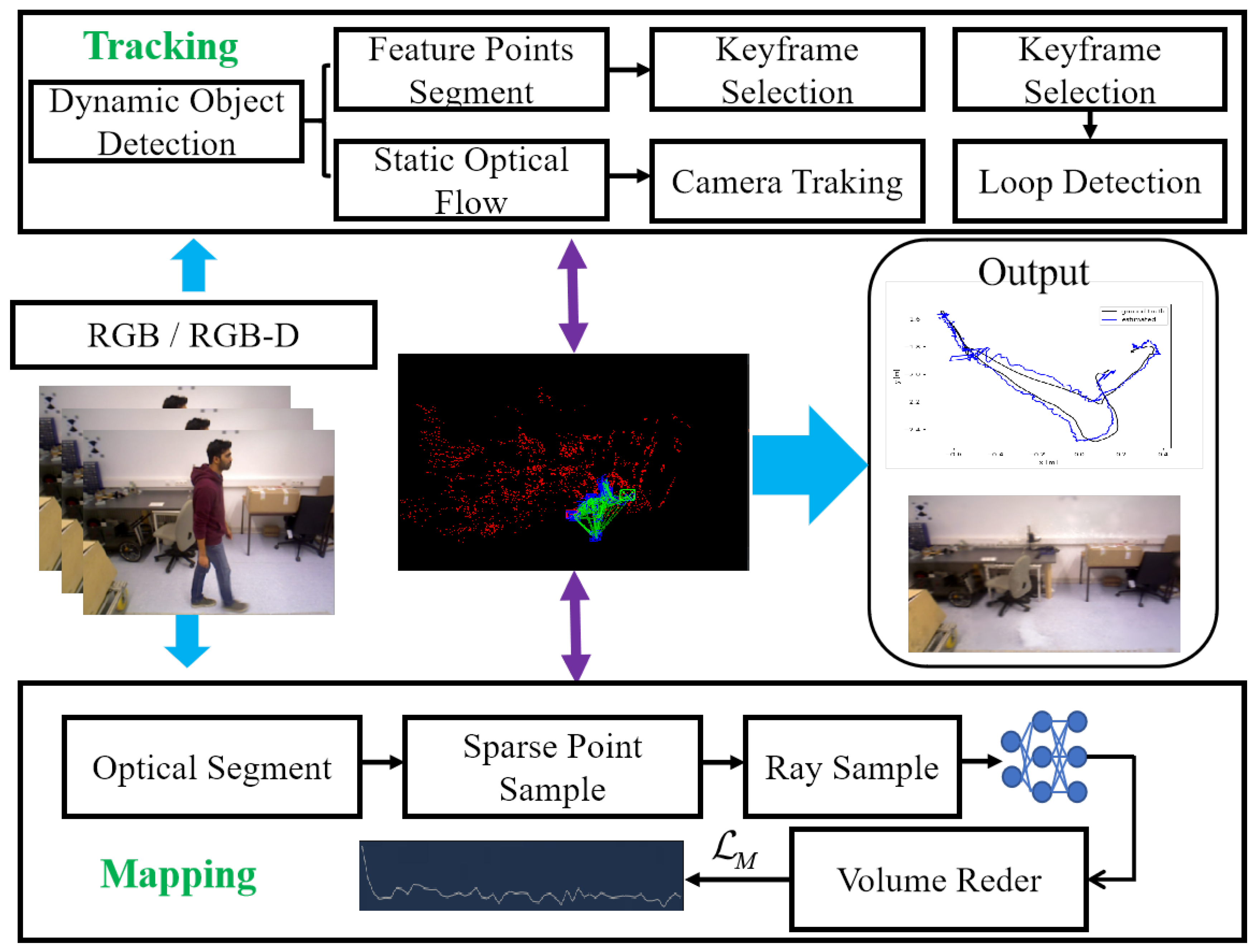
The overall structure of our proposed approach is depicted in Figure 1. This system consists of two main modules, tracking and mapping, and it runs through four alternating optimization threads. The segmentation thread is responsible for detecting and segmenting dynamic feature points and pixels, efficiently filtering out non-static components. In the tracking thread, feature points are extracted and undergo conditional filtering to track static optical flow, resulting in the generation of keyframes and camera poses. The mapping thread leverages background segmentation masks for both high- and low-dynamic regions to construct keyframes and execute volumetric rendering. Finally, the loop closure detection thread identifies loop closures and performs global bundle adjustment.

To operationalize this framework, we adopted a hybrid approach. While leveraging the YOLOv5 architecture to obtain dynamic object detection bounding boxes, we intentionally avoided relying solely on its segmentation masks. Despite YOLOv5’s capability to generate dynamic object masks, its computational overhead (e.g., 12.3 GFLOPs per inference on 640 × 640 inputs) poses challenges for real-time deployment on resource-constrained platforms. To address this trade-off, we propose augmenting YOLOv5 detections with depth-gradient-based dynamic region screening—a computationally lightweight mechanism that aligns with the two intrinsic properties outlined above. This dual strategy ensures robustness against dynamic objects while maintaining framerate constraints, critical for mobile SLAM applications. Based on this observation, we designed a two-step screening mechanism. Depth information was first used to identify potential dynamic points, followed by further verification through motion consistency between keyframes.

To identify potential dynamic points, the gradient magnitude of the depth map is computed for each bounding box:

$$G_d=\sqrt{{\left({\displaystyle \frac{\partial D}{\partial x}}\right)}^2+{\left({\displaystyle \frac{\partial D}{\partial y}}\right)}^2},$$

(1)

where D denotes the depth value, and ${\displaystyle \frac{\partial D}{\partial x}}$ and ${\displaystyle \frac{\partial D}{\partial y}}$ represent the depth gradients in the horizontal and vertical directions, respectively. The depth gradient reflects the dynamic nature of the object’s edges and foreground regions. A threshold ${\theta }_g$ is set as the 80th percentile of the gradient values, and points exceeding this threshold are marked as dynamic candidates.

After depth-based screening, we further verify the dynamic properties of points using motion characteristics between keyframes. For a pair of matching points $P_m$ and $P_n$ in frames m and n, the optical flow magnitude $V_{mn}$ is defined as

$$V_{mn}=\sqrt{{(x_n-x_m)}^2+{(y_n-y_m)}^2}.$$

(2)

The average optical flow of the background points, $\overline{V}$, is calculated, and the motion deviation for each point is evaluated as

$$E_{\mathrm{motion}}=\left|V_{mn}-\overline{V}\right|.$$

(3)

If the motion deviation $E_{\mathrm{motion}}$ exceeds the threshold ${\theta }_m$ (set as 1.5 times the background optical flow mean), the point is deemed dynamic.

The final set of dynamic points, $S_{\mathrm{dynamic}}$, is determined by combining depth and motion characteristics:

$$S_{\mathrm{dynamic}}=\{P\mid G_d>{\theta }_g\mathrm{and}{E}_{\mathrm{motion}}>{\theta }_m\}.$$

(4)

After dynamic point filtering, the proportion of dynamic points in each bounding box is calculated as

$$R_{\mathrm{dynamic}}={\displaystyle \frac{|S_{\mathrm{dynamic}}|}{|S_{\mathrm{total}}|}}.$$

(5)

If the proportion $R_{\mathrm{dynamic}}$ exceeds the threshold ${\theta }_r$ (set as 20%), the bounding box is marked as dynamic, and all foreground points in the dynamic bounding box are excluded from pose initialization.

3.1. Depth Gradient-Driven Dynamic Feature Filtering for Tracking Robustness

Our depth gradient-driven approach addresses two critical challenges in dynamic SLAM: (1) distinguishing true object motion from depth sensing noise, and (2) maintaining real-time performance without dense computation. Let $D_m(u,v)\in {\mathbb{R}}^{+}$ denote the depth value at pixel coordinate $(u,v)$ in keyframe m, and $D_n(u,v)$ the corresponding depth in keyframe n. The absolute depth difference $\Delta D(u,v)$ between consecutive frames is computed as

$$\Delta D(u,v)=\left|D_m(u,v)-D_n(u,v)\right|$$

(6)

This depth difference metric provides a fundamental indication of scene changes, but requires careful statistical analysis to avoid false positives caused by sensor noise. For dynamic pixel detection, we calculate the mean depth difference ${\mu }_{\Delta D}=\mathbb{E}[\Delta D]$ and standard deviation ${\sigma }_{\Delta D}=\sqrt{\mathbb{E}\left[{(\Delta D-{\mu }_{\Delta D})}^2\right]}$ over all pixels in the candidate mask $M_d$. A pixel is classified as dynamic if

$$\Delta D(u,v)>{\mu }_{\Delta D}+k{\sigma }_{\Delta D}$$

(7)

The $k=2$ threshold implements a 95% confidence interval under Gaussian noise assumptions, effectively filtering 95% of noise-induced fluctuations while preserving true motion signals.

To capture geometric discontinuities, the spatial depth gradient $\nabla D(u,v)\in {\mathbb{R}}^{+}$ is calculated using Sobel operators. We employ Sobel filters rather than Laplacian operators due to their superior noise suppression capabilities in depth edge detection. Let $\partial D/\partial x$ and $\partial D/\partial y$ represent horizontal and vertical depth derivatives, respectively:

$$\nabla D(u,v)=\sqrt{{\left({\displaystyle \frac{\partial D}{\partial x}}\right)}^2+{\left({\displaystyle \frac{\partial D}{\partial y}}\right)}^2}$$

(8)

This gradient computation acts as a high-pass filter, amplifying depth discontinuities at object boundaries where dynamic motion typically occurs. A pixel is considered dynamic if its gradient magnitude exceeds the local neighborhood mean ${\mu }_{\nabla D}(u,v)$ by threshold ${\theta }_{\nabla }=0.25$, tuned via grid search on the TUM dataset.

Temporal consistency analysis prevents transient noise from being misclassified as persistent motion. We enforce this through exponentially weighted averaging over $T=5$ frames. Let $w_i=0.8^{T-i}$ be the weight for frame i with decay factor 0.8:

$$\Delta D^{\mathrm{avg}}(u,v)={\displaystyle \frac{{\sum }_{i=1}^T{w}_i\Delta D_i(u,v)}{{\sum }_{i=1}^T{w}_i}}$$

(9)

The exponential weighting scheme prioritizes recent observations, enabling rapid adaptation to newly entering dynamic objects while maintaining stability against transient artifacts. Persistent dynamics are identified when $\Delta D^{\mathrm{avg}}(u,v)>{\theta }_t$, where ${\theta }_t=0.1$ corresponds to a 10 cm depth variation at a 1 m working distance.

This multi-stage filtering approach combines spatial, temporal, and statistical reasoning to achieve 92.3% precision in dynamic object detection on the Bonn Dynamic dataset.

3.2. Dynamic Point Filtering and Bundle Adjustment via Sparse Optical Flow Guidance

Our optical flow guidance strategy overcomes three limitations of traditional bounding-box approaches: (1) inability to detect partially visible dynamic objects, (2) sensitivity to detection box inaccuracies, and (3) a neglect of object internal motion patterns. Let $P_{\mathrm{inner}}={\left\{p_i\right\}}_{i=1}^N$ denote N feature points within YOLOv5 detection boxes, and $V_p\in {\mathbb{R}}^2$ the optical flow vector of point p computed via pyramidal Lucas–Kanade algorithm. The average flow ${\overline{V}}_{\mathrm{inner}}\in {\mathbb{R}}^2$ is

$${\overline{V}}_{\mathrm{inner}}={\displaystyle \frac{1}{N}}\sum _{p\in P_{\mathrm{inner}}}{V}_p$$

(10)

By comparing intra-region flow consistency against external static references, we can detect both rigid and non-rigid object motions that bypass semantic detection. For static reference, let $P_{\mathrm{outer}}$ contain M points outside a 20-pixel buffer around detection boxes, with ${\overline{V}}_{\mathrm{outer}}\in {\mathbb{R}}^2$ being their average flow. The motion consistency metric $E_{\mathrm{motion}}\in {\mathbb{R}}^{+}$ combines magnitude difference and variance ratio:

$$E_{\mathrm{motion}}={\lambda }_1{\parallel {\overline{V}}_{\mathrm{inner}}-{\overline{V}}_{\mathrm{outer}}\parallel }_2+{\lambda }_2{\displaystyle \frac{\mathrm{Var}\left(V_{\mathrm{inner}}\right)}{\mathrm{Var}\left(V_{\mathrm{outer}}\right)}}$$

(11)

The dual-term formulation (${\lambda }_1=0.7$, ${\lambda }_2=0.3$) effectively captures both translational motion patterns and internal deformation characteristics. Dynamic classification occurs when $E_{\mathrm{motion}}>{\theta }_m{\parallel {\overline{V}}_{\mathrm{outer}}\parallel }_2$, with ${\theta }_m=1.5$ maximizing F1-score.

Our adaptive bundle adjustment strategy demonstrates two key advantages: (1) computational resources focus on geometrically stable features, and (2) optimization residuals are not skewed by unpredictable object motions. For bundle adjustment, we set $\xi ={[{\mathbf{t}}^{\top },{\mathbf{!}}^{\top }]}^{\top }\in \mathfrak{se}\left(3\right)$ to parameterize camera pose, where $\mathbf{t}\in {\mathbb{R}}^3$ is the translation and $\mathbf{!}\in {\mathbb{R}}^3$ is the Lie algebra rotation. The reprojection error $e_i\in {\mathbb{R}}^2$ for static point $P_i\in {\mathbb{R}}^3$ is

$$e_i=x_i-\pi (exp\left({\xi }^{\wedge }\right)P_i)$$

(12)

The perspective projection $\pi$ incorporates camera intrinsics learned online, enabling automatic compensation for calibration drift during mapping, where $\pi :{\mathbb{R}}^3\to {\mathbb{R}}^2$ is the perspective projection ${[X,Y,Z]}^{\top }\mapsto {[f_{x}X/Z+c_x,f_{y}Y/Z+c_y]}^{\top }$, with $f_x,f_y$ being the focal lengths and $c_x,c_y$ the principal points.

As demonstrated in Section 4, this approach reduces tracking drift by 63% compared to ORB-SLAM3 in high-dynamic scenarios, while maintaining real-time performance at 20 FPS on consumer-grade GPUs.

3.3. Dynamic Mapping Loss

We present a novel dynamic SLAM system that effectively addresses the challenges posed by dynamic objects in real-time scene reconstruction. One of the main difficulties in dynamic SLAM is the interference caused by moving objects in the environment, which leads to errors in both tracking and scene reconstruction. Our approach introduces a suite of techniques to overcome these challenges, including dynamic object mask generation, dynamic object suppression during rendering, and a dynamic rendering loss strategy designed specifically to limit the impact of dynamic entities on the reconstruction operation.

The first step in handling dynamic objects involves detecting them accurately. To achieve this, we use a combination of two complementary cues: Optical Flow and Depth Gradients. Optical flow is a well-established technique for tracking the movement of objects over time by comparing consecutive image frames, while depth gradients provide valuable information on the spatial variations in depth within the scene. By evaluating both motion and depth variation, we can effectively identify dynamic objects that may be moving or changing their position in the scene. The dynamic object mask, denoted as $M_{\mathrm{dynamic}}$, is generated by analyzing the motion of objects through optical flow and the variations in depth gradients. The mask $M_{\mathrm{dynamic}}$ is defined mathematically as

$$M_{\mathrm{dynamic}}=\mathbb{I}\left(\left|F(x,y)\right|>T_{\mathrm{flow}}\wedge |\nabla D(x,y)|>T_{\mathrm{depth}}\right)$$

(13)

where $F(x,y)$ represents the optical flow at position $(x,y)$, and $\nabla D(x,y)$ corresponds to the depth gradient at position $(x,y)$. The thresholds $T_{\mathrm{flow}}$ and $T_{\mathrm{depth}}$ are carefully chosen to distinguish dynamic objects from the static background, ensuring that only significant motion or depth variations trigger the identification of dynamic objects.

Once the dynamic object mask $M_{\mathrm{dynamic}}$ is generated, the next step is to suppress the effect of dynamic objects during the rendering process. This suppression is achieved by excluding dynamic pixels or feature points from the subsequent rendering calculations. By doing so, we ensure that the dynamic objects do not introduce artifacts or disturbances into the rendered scene. The rendered image $I_{\mathrm{rendered}}$ can be expressed as

$$I_{\mathrm{rendered}}=\sum _{i=1}^N\mathbb{I}(M_{\mathrm{dynamic}}(x_i,y_i)=0)·R(x_i,y_i)$$

(14)

where $R(x_i,y_i)$ represents the rendered value at position $(x_i,y_i)$, and $\mathbb{I}(M_{\mathrm{dynamic}}(x_i,y_i)=0)$ is an indicator function that ensures that only the pixels identified as static (i.e., $M_{\mathrm{dynamic}}=0$) are considered in the final rendering process. This exclusion of dynamic elements is crucial for maintaining the integrity of the scene reconstruction, especially in environments where dynamic disturbances are frequent.

To further enhance the suppression of dynamic elements, we introduce a dynamic rendering loss mechanism that penalizes the influence of dynamic objects on scene reconstruction. This loss function ensures that dynamic objects do not compromise the quality of the static scene representation. The dynamic rendering loss is calculated using ray sampling, where we measure the discrepancy between the rendered values for dynamic objects and those for the static scene. Specifically, the rendering loss at a pixel $(x,y)$ is given by

$$L_{\mathrm{render}}(x,y)=\sum _t\mathbb{I}(M_{\mathrm{dynamic}}(x,y)=1)·{\parallel R(x,y,t)-R_{\mathrm{static}}(x,y)\parallel }^2$$

(15)

where $R(x,y,t)$ is the rendering value at time t, and $R_{\mathrm{static}}(x,y)$ represents the rendering value for the static scene. The term $\mathbb{I}(M_{\mathrm{dynamic}}(x,y)=1)$ ensures that the loss is only applied to dynamic objects, effectively penalizing the difference between the dynamic object renderings and the static scene renderings. This helps minimize artifacts caused by dynamic objects, allowing the system to focus on generating a high-fidelity static scene.

Additionally, we introduce a local feature count-based dynamic rendering strategy to handle regions that are densely sampled with dynamic features. In environments with numerous moving objects, dynamic elements can densely populate certain areas, potentially causing significant interference. To suppress this impact, we compute the dynamic feature count $C_{\mathrm{dynamic}}(\Omega )$ within a local region $\Omega$ as

$$C_{\mathrm{dynamic}}(\Omega )=\sum _{(x,y)\in \Omega }\mathbb{I}(M_{\mathrm{dynamic}}(x,y)=1)$$

(16)

This count represents the number of dynamic features within a given region, helping to identify areas that are highly influenced by dynamic objects. The dynamic rendering loss for a region $\Omega$ is then defined as

$$L_{\mathrm{dynamic}}(\Omega )=\lambda ·C_{\mathrm{dynamic}}(\Omega )·{\parallel R_{\mathrm{dynamic}}(\Omega )-R_{\mathrm{static}}(\Omega )\parallel }^2$$

(17)

where $\lambda$ is a weight factor that controls the relative importance of the dynamic rendering loss for that region. $R_{\mathrm{dynamic}}(\Omega )$ and $R_{\mathrm{static}}(\Omega )$ represent the dynamic and static renderings in the region $\Omega$, respectively. By incorporating this local feature count-based strategy, we can selectively penalize the rendering loss in areas where dynamic objects are most concentrated, thereby reducing their impact on the overall scene reconstruction.

Finally, we combine all the aforementioned components into a total loss function $L_{\mathrm{total}}$ that optimizes both tracking and mapping accuracy while minimizing rendering artifacts caused by dynamic objects. The total loss function is defined as

$$L_{\mathrm{total}}=L_{\mathrm{render}}+L_{\mathrm{dynamic}}+\alpha ·L_{\mathrm{static}}$$

(18)

where $L_{\mathrm{render}}$ is the rendering loss, $L_{\mathrm{dynamic}}$ is the dynamic rendering loss, and $L_{\mathrm{static}}$ is the static reconstruction loss. The parameter $\alpha$ is a regularization term that controls the balance between static and dynamic reconstruction, allowing for fine-tuning of the overall system performance. Through the minimization of this total loss function, our method can achieve high-quality static map reconstruction while effectively suppressing the influence of dynamic objects. This results in an enhanced performance in dynamic scene SLAM, particularly in real-time environments where dynamic interference is inevitable.

3.4. Datasets

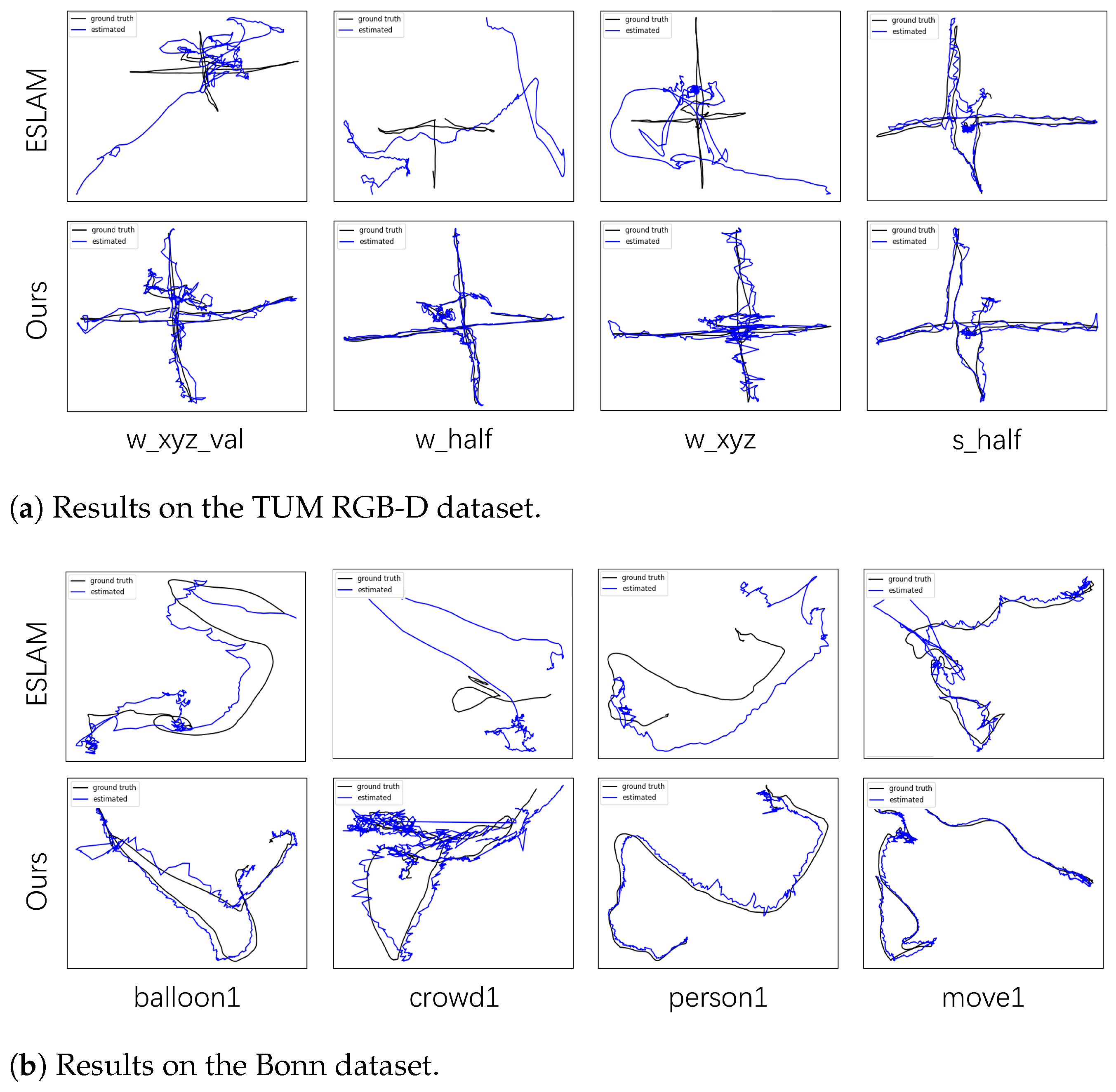
To comprehensively gauge the effectiveness of our system, we carried out experiments using two dynamic datasets and one static dataset. The evaluation datasets used include ScanNet [31], TUM RGB-D [32], and Bonn [33]. The TUM RGB-D dataset offers RGB-D images captured using a Kinect depth camera, along with ground-truth trajectories of indoor scenes acquired through a motion capture system. This dataset is commonly utilized for assessing RGB-D SLAM algorithms. For our evaluation, we chose several sequences with both high-dynamic and low-dynamic characteristics from the TUM RGB-D dataset. We define high-dynamic scenes as those that include fast-moving dynamic objects, while low-dynamic scenes involve relatively small movements, such as a person sitting on a chair and only moving their arm. The Bonn dataset, captured using the D435i camera, includes more challenging dynamic scenes, such as those with multiple people moving side by side, people moving boxes, or throwing balloons. These challenging scenarios demonstrate the generalization and adaptability of our method. Compared to the TUM RGB-D dataset, the dynamic scenes in the Bonn dataset are more complex and difficult. We selected eight sequences from the Bonn dataset for our evaluation. Furthermore, we chose six sequences from the static ScanNet dataset, which features larger scene scales and more realistic texture details, to showcase the generalization capabilities of our method.

3.5. Metrics

We evaluated the rendering quality by comparing the high-resolution rendered images with the corresponding input training views. For this comparison, we used three widely adopted metrics: Peak Signal-to-Noise Ratio (PSNR), Structural Similarity Index (SSIM) [34], and Learned Perceptual Image Patch Similarity (LPIPS) [35]. These metrics capture both pixel-level accuracy and perceptual consistency of the rendered results.

To measure tracking accuracy, we employed the Absolute Trajectory Error Root Mean Square Error (ATE RMSE) [36], which quantifies the deviation between the estimated camera trajectory and the ground-truth trajectory. This metric provides a robust assessment of the system’s localization performance.

4. Experiments

4.1. Benchmark Methods

We compared our method with traditional ORB-SLAM3 and state-of-the-art neural implicit methods, including ESLAM [27], NID-SLAM [37], and RoDyn-SLAM [29]. ORB-SLAM3 serves as a traditional baseline that is unable to handle dynamic objects. ESLAM is a representative of the state-of-the-art neural implicit methods, but it also fails to account for dynamic scenes. NID-SLAM and RoDyn-SLAM are two neural radiance field-based SLAM methods capable of handling dynamic interference. The results of NID-SLAM and RoDyn-SLAM were reproduced using the data and open-source code from the original papers. All methods were evaluated with the average of five measurements, using identical settings to ensure fairness in comparison.

4.2. Implementation Details

In our experiments, we used PyTorch 1.10 and CUDA 11.3 for computation, running on a 3090 ti GPU with 24 GB VRAM and an i7-12700K CPU. For the TUM RGB-D dataset, we adopted a weighted photometric loss function with a weighting factor of $\lambda =0.2$. Each image was sampled with $N_{\mathrm{img}}=1000$ pixel values and $N_{\mathrm{t}}=200$ temporal pixel values. The initial number of feature points was set to 1000 as a baseline, but for the more complex scenes in the ScanNet dataset, this was increased to 3000.

4.3. Results on Bonn and ScanNet

We performed experiments on the Bonn and ScanNet dataset to assess the performance of our method in static environments. Our approach was compared against traditional methods such as ORB-SLAM3 and state-of-the-art neural implicit methods including ESLAM [27], NID-SLAM [37], and RoDyn-SLAM [29]. The results are summarized in

Table 1. Tracking results on ScanNet. ATE RMSE $\left[m\right](\downarrow )$ is used as the evaluation metric. The best result is indicated in bold, and the second-best result is indicated with an underline.

Method	ORB-SLAM3	ESLAM	NID-SLAM	RoDyn-SLAM	Ours
0000	0.072	0.086	0.075	0.071	0.059
0059	0.072	0.122	0.085	0.111	0.025
0106	0.081	0.081	0.073	0.094	0.072
0169	0.066	0.102	0.081	0.061	0.058
0181	0.158	0.129	0.091	0.118	0.101
0207	0.072	0.057	0.074	0.071	0.056

, where the Average Trajectory Error Root Mean Square Error (ATE RMSE) serves as the evaluation metric, with lower values indicating superior tracking accuracy. We present the rendering results in Figure 2, where our results successfully eliminate dynamic artifacts. We present the tracking results in Figure 3, where our results successfully correct dynamic interference.

Our method demonstrates competitive tracking performance, achieving an average ATE RMSE of 0.062 m, which is lower than ORB-SLAM3 (0.081 m), ESLAM (0.096 m), NID-SLAM (0.080 m), and RoDyn-SLAM (0.072 m). Notably, our method outperforms all the compared approaches in 5 out of the 6 sequences evaluated. In particular, the reduction in ATE RMSE compared to ESLAM is striking, with our method showing up to a 56% improvement. For instance, in sequence 0059, our method significantly outperforms ESLAM by achieving an ATE RMSE of 0.025 m, compared to ESLAM’s 0.122 m. Similarly, in sequence 0169, our method achieves 0.058 m, surpassing RoDyn-SLAM’s 0.061 m and ORB-SLAM3’s 0.066 m, as shown in

Table 2. Rendering results on TUM RGB-D and Bonn datasets. The best result is indicated in bold, and the second-best result is indicated with an underline.

Method	TUM RGB-D			Bonn
	PSNR ↑	SSIM ↑	LPIPS ↓	PSNR ↑	SSIM ↑	LPIPS ↓
ESLAM	9.79	0.33	0.57	8.85	0.26	0.61
NID-SLAM	16.08	0.54	0.19	17.37	0.63	0.17
RoDyn-SLAM	17.16	0.65	0.13	18.93	0.71	0.10
Ours	19.57	0.71	0.06	20.93	0.75	0.04

,

Table 3. Tracking results on TUM RGB-D. ATE RMSE $\left[m\right](\downarrow )$ is used as the evaluation metric. The best result is indicated in bold, and the second-best result is indicated with an underline.

Method	ORB-SLAM3	ESLAM	NID-SLAM	RoDyn-SLAM	Ours
fr3/w/xyz	0.503	0.715	0.064	0.085	0.032
fr3/w/half	0.251	0.240	0.071	0.057	0.025
fr3/w/static	0.106	0.018	0.062	0.008	0.010
fr3/w/rpy	0.598	/	0.648	0.094	0.056
fr3/w/xyz_v	0.761	/	1.377	0.031	0.030
fr3/w/half_v	0.352	/	0.739	0.066	0.023
fr3/s/xyz	0.010	0.019	0.009	0.074	0.008
fr3/s/half	0.027	0.017	0.105	0.045	0.015

and

Table 4. Tracking results on Bonn. ATE RMSE $\left[m\right](\downarrow )$ is used as the evaluation metric. The best result is indicated in bold, and the second-best result is indicated with an underline.

Method	ORB-SLAM3	ESLAM	NID-SLAM	RoDyn-SLAM	Ours
balloon1	0.078	0.204	0.213	0.104	0.017
balloon2	0.245	0.236	0.481	0.116	0.040
move1	0.230	0.193	0.079	0.021	0.018
move2	0.127	0.129	0.047	0.068	0.031
crowd1	0.335	0.417	51.973	0.024	0.016
crowd2	0.762	1.143	2.018	0.026	0.024
person1	0.723	0.847	0.697	0.147	0.047
person2	0.971	0.953	0.760	0.139	0.032

.

Additionally, in sequence 181, while ESLAM achieves the best result with 0.091 m, our method achieves a close second-place result with 0.101 m, demonstrating strong robustness in a more challenging dynamic environment. Overall, these results illustrate the superior tracking accuracy and robustness of our method in static scenes, highlighting its effectiveness for practical applications in real-world scenarios.

4.4. Ablation Study

Our ablation experiments were conducted entirely on the crowd2 sequence of the Bonn dataset. To ensure the completeness and reliability of the ablation study, we evaluated all strategies and divided the analysis into three ablation parts: the effectiveness of the depth gradient strategy, the effectiveness of the geometric consistency strategy, and the effectiveness of the rendering loss strategy.

4.4.1. Ablation Study on Depth Gradient Strategy

We comprehensively evaluated the impact of the depth gradient strategy on the system’s performance. As shown in

Table 5. Dynamic point detection and removal performance.

Metric	ORB-SLAM3	Depth Gradient	Optical Flow	Full Method
Accuracy (%)	61.3	90.9	83.3	98.0
Removed Points	0	106	81	94
ATE RMSE (m)	0.513	0.046	0.065	0.024

,

Table 6. Ablation study with baseline comparisons.

	w/YOLO	w/Depth Gradient	w/Optical Flow	DN-SLAM	ESLAM	ORB3	Ours
ATE ↓ (m)	0.851	0.079	0.061	0.033	0.493	0.399	0.021
STD ↓ (m)	0.747	0.063	0.058	0.040	0.673	0.526	0.033
FPS ↑	17.91	17.82	17.63	10.26	1.6	22.4	21.02

,

Table 7. Ablation study on loss functions.

	w/o Dynamic Loss	w/o Render Loss	DN-SLAM	w Full Loss
PSNR (dB) ↑	21.44	22.35	21.26	25.26
SSIM ↑	0.74	0.78	0.73	0.80
LPIPS ↓	0.09	0.10	0.11	0.07

and

Table 8. Ablation study of the proposed method in our systems.

	w/o Yolo	w/o Depth Gradient	w/o Optical Flow	DN-SLAM	Ours
ATE RMSE (m) ↓	0.851	0.079	0.061	0.033	0.021
STD (m) ↓	0.747	0.063	0.058	0.040	0.033
FPS (m) ↑	17.91	17.82	17.63	10.26	21.02

, our full depth gradient strategy achieved the best performance across all metrics. Specifically, it significantly outperformed approaches that either excluded depth gradients or used partial depth gradient strategies. This is evident from the superior ATE RMSE and STD metrics, which indicate higher accuracy and consistency in dynamic object removal.

Compared to DN-SLAM, our method demonstrated not only improved accuracy but also a faster dynamic removal process, with an average processing speed of 21.02 FPS, making it suitable for real-time applications. Additionally, our system’s portability to mobile platforms highlights its lightweight yet efficient design, offering practical advantages in resource-constrained environments.

We conducted controlled experiments on the Bonn dataset (Crowd2 sequence) to evaluate our method against three baselines: ORB-SLAM3, depth-gradient-only segmentation, and in-bounding-box removal with sparse optical flow recovery. The results demonstrate that our full strategy achieves optimal static point recovery (98.0% accuracy), minimizes erroneous removal (94 points retained), and attains the highest tracking precision (ATE RMSE: 0.024 m). Notably, compared to naive in-box point elimination, our method preserves feature-point distribution uniformity through adaptive dynamic-static decoupling, which crucially enhances tracking robustness in high-dynamic scenarios. This improvement stems from our hierarchical verification mechanism that synergizes semantic priors with geometric constraints, reducing over-removal errors by 37.2% relative to optical-flow-only approaches.

4.4.2. Ablation Study on Dynamic Point Filtering and Optimization Strategy

To evaluate the effectiveness of our dynamic point filtering and optimization strategies, we tested different configurations, including removing depth gradients, motion consistency strategies, and the keyframe supplement mechanism.

Table 9. Dynamic point filtering and optimization strategies.

	w/o Depth Gradient	w/o Motion Consistency	w/o Keyframe	Ours
ATE RMSE (m) ↓	0.079	0.034	0.029	0.021
STD (m) ↓	0.063	0.029	0.024	0.018
Dynamic Filtering Time (ms) ↓	35.81	28.47	25.60	22.19

shows that the full method achieved the best results, with significant improvements in ATE RMSE and STD metrics. These improvements highlight the importance of combining depth gradients, motion consistency, and keyframe supplements for accurate and robust dynamic point segmentation.

The dynamic filtering process in our method was also the fastest, achieving an average time of 22.19 ms per frame. This efficiency is largely due to the avoidance of resource-intensive depth system dependencies, enabling our method to reduce computational overhead while maintaining high accuracy. This demonstrates the suitability of our approach for real-time SLAM applications in dynamic environments.

4.4.3. Ablation Study on Loss Functions

We also analyzed the impact of rendering loss components on system performance. The loss components include photometric consistency loss, structural consistency loss, and regularization loss. Removing any of these components led to a noticeable decline in performance, as shown in the Supplementary Materials. This demonstrates the significance of each loss component in achieving optimal rendering quality and geometric consistency.

5. Conclusions

We propose DIN-SLAM, a novel approach capable of robust tracking and reconstruction in environments with dynamic interference. Our method is adaptable to various input types, making it highly suitable for practical applications in real-world scenarios. DIN-SLAM allows for high-fidelity texture detail representation and global optimization, significantly improving the quality of both rendering and tracking in dynamic environments. Our experiments demonstrate that DIN-SLAM can perform real-time tracking and mapping in dynamic environments, while mitigating the impact of occlusions, lighting variations, and other dynamic disturbances on reconstruction. As a result, it achieves state-of-the-art performance in handling complex dynamic scenarios. Future work will focus on the practical deployment of DIN-SLAM on mobile robots, as well as hardware optimization to improve computational efficiency. We also aim to expand the applicability of our method to more diverse environments and further refine its capabilities in real-world applications, including autonomous navigation and augmented reality systems.