High-Fidelity Modeling and Stability Analysis of Microgrids by Considering Time Delay

Abstract

Microgrids (MGs) offer substantial environmental, economic, and technological benefits by supplying electrical energy to the grid or local consumers via power electronic inverter-interfaced Distributed Energy Resources (DERs). However, the design, control, and stability analysis of inverter-interfaced MGs present significant challenges, as numerous system parameters influence the overall stability of these MGs. While extensive research has been conducted on MG stability, predominantly through eigenvalue-based state-space models, further refinement is necessary for more accurate stability assessments. This paper provides an accurate and detailed stability analysis of MGs, focusing specifically on parallel-connected grid-forming inverters (GFIs) operating in island mode. The novelty of this paper lies in three key contributions: (1) accurately considering a time delay in regard to the dq-axis synchronous reference frame, (2) the enhanced accuracy of the small-signal model for the purpose of the voltage control loop, and (3) the enhanced accuracy of the small-signal model for the purpose of the current control loop. In the literature, digital control-induced time delays are typically incorporated directly into the dq-axis, while the effect of the phase shift is then neglected, leading to inaccurate stability assessment results. Accordingly, the motivation of this paper is to consider the time delay, which naturally exists in regard to the abc-axis, and accurately represent it in regard to the dq-axis by modeling the phase shift effect for precise stability analysis. These contributions enable a precise small-signal model to be developed and eigenvalue-based stability analysis to be carried out by not only incorporating an accurate representation of the time delay, but also considering the voltage control loop and the current control loop in regard to the dq-axis synchronous reference frame. To achieve this aim, a full-order state-space and small-signal model of GFIs is developed, considering all the subsystem dynamics. The theoretical analysis conducted within the MATLAB m-file code environment (other programming languages, such as C or Python, could also be employed) and the real-time simulation results obtained using PLECS show excellent agreement, verifying the accuracy of the proposed method and highlighting its superior precision compared to conventional stability analysis. The real-time simulation results show that the proposed small-signal model has less than 5% deviation in regard to both active and reactive power droop coefficient limits, while the conventional model deviates by 22% and 530% in regard to active and reactive power droop, respectively. Consequently, this study determines the critical boundaries of the control parameters that ensure MG stability, providing a more accurate foundation for stability analysis and control design.

1. Introduction

Microgrids (MGs) are versatile electrical power systems that can operate either as part of a larger grid or independently as self-sustaining power sources. These systems consist of small-scale renewable and/or conventional inverter-interfaced Distributed Energy Resources (DERs), supplying electricity to nearby loads. The design and control of MGs are of significant importance in regard to maintaining stable and reliable operation. Given the increasing penetration of inverter-interfaced DERs, maintaining small-signal stability is crucial to prevent instabilities in MGs. This paper addresses this challenge by accurately incorporating time delay effects into the dq-axis synchronous reference frame and enhancing the small-signal modeling of both voltage and current control loops. These advancements enable more precise eigenvalue-based stability analysis, improving the understanding of the dynamic behavior of inverter-based MGs.

Small-signal stability is defined as the ability of a system to maintain stable operation by returning to a specific operating point following small disturbances, such as load variations or changes in the operating point. The reliability of the stability analysis depends on the accuracy of the modeling of the entire system. In island MGs, DERs are commonly interfaced with inverter topologies. Inverters used in MGs are generally classified into three main categories based on their functionality: (i) grid-forming inverters (GFIs), (ii) grid-feeding inverters, and (iii) grid-supporting inverters. Grid-feeding and grid-supporting inverters operate in grid-connected mode, supplying power to the main grid, while also contributing to voltage and frequency stability [1]. In contrast, GFIs are designed to provide power to local loads independently of the main grid, functioning in what is often referred to as island mode. These GFIs, also known as island inverters, derive their reference voltage and frequency from primary control mechanisms, allowing them to operate autonomously without requiring the main grid for the purposes of the reference voltage and frequency. In island microgrids (MGs), grid-forming inverters (GFIs) are connected to the point of common coupling (PCC) and operate in parallel, allowing electrical energy from single or multiple sources to be delivered to loads through multiple GFIs. Island MGs offer several advantages, including increased power capacity, enhanced redundancy, and improved operational reliability [2,3]. However, island MGs require a complex approach in regard to their analysis and design. The key aspects of this approach include stability analysis [4], synchronization systems [5], protection mechanisms [3], power management [6], power quality [7,8], and feedback control [9]. To ensure efficient operation and compliance with the relevant standards [10], island MGs must employ a multi-functional closed-loop control system. This system should be capable of regulating the voltage and frequency, ensuring accurate power sharing, synchronizing with or isolating from the main grid, managing the power flow, and optimizing the operating costs. These operational demands have driven the development of a hierarchical control system for MGs, typically structured into zero-level [11,12,13], primary [14,15], secondary, and tertiary control layers [16,17]. This paper focuses specifically on the zero-level and primary control of island MGs.

Zero-level control in island microgrids (MGs) encompasses the voltage controller, current controller, decoupling scheme, and feed-forward (FF) control mechanisms. In contrast, the primary control system is responsible for managing power sharing among parallel-connected grid-forming inverters (GFIs). It provides reference voltage and frequency values to the zero-level control, enabling each GFI to distribute active and reactive power according to its rated power capacity [14]. Droop-based control methods are often favored in regard to primary control systems due to their flexibility, ease of integrating new distributed energy sources, redundancy, and straightforward implementation, making them more reliable than communication-based approaches. However, despite these advantages, droop-based control has its limitations, such as frequency and voltage deviations, as well as degraded reactive power quality due to output impedance mismatches. As a result, conventional droop control alone may not be sufficient to achieve optimal performance. To address these issues, extensive research has been conducted on various modifications of droop-based control to enhance power sharing in island MGs [18,19,20,21,22]. One widely adopted solution is the use of the virtual impedance concept, combined with conventional droop control. This approach has garnered significant attention for its ability to mitigate power quality challenges, such as improving stability, compensating for output impedance mismatches, handling unbalanced loads, and addressing harmonic distortions [23,24]. The stability of island microgrids (MGs) is a critical concern, even more so than in traditional power systems, as MGs operate independently and must maintain their own stability. In traditional power systems, the inertia provided by large generators plays a key role in damping voltage and frequency oscillations. However, in MGs, distributed generation (DG) units are connected to the grid via inverters, making them more vulnerable to voltage and frequency oscillations than traditional systems. This heightened sensitivity can lead to instability in island MGs [25,26].

Small-signal stability analysis has long been a powerful tool for assessing the stability of MGs. In the literature, small-signal stability analysis for island MGs is typically divided into the modeling of low-frequency and high-frequency dynamics, corresponding to primary control and zero-level control, respectively [4]. Thus, small-signal stability studies are generally divided into two main categories: (i) the small-signal modeling of primary control, with a focus on droop-based control, and (ii) the small-signal modeling of zero-level control, which falls within the scope of this paper. A comprehensive literature review is presented as follows.

Stability analysis based on primary control (low-frequency dynamics): Stability analysis involving conventional droop control, specifically through small-signal modeling of primary control, was first introduced in [27] for parallel-connected single-phase inverters. The study identified that the droop control parameters, namely the active power droop coefficient, reactive power droop coefficient, and power filter cut-off frequency, are the most critical factors influencing system stability. In [28], a small-signal analysis of an adaptive decentralized droop controller was conducted, although it overlooked zero-level control schemes. A new small-signal model for synchronverters, designed to emulate synchronous generators, was proposed in [29], while [30] introduced a small-signal model for microgrids (MGs) based on universal droop control. In [31], the stability margin of a droop-controlled island MG was enhanced using cascaded lead compensators, with small-signal analysis validating its effectiveness.

Additionally, ref. [32] presented a novel small-signal model that considered the dynamic interactions between the inverters due to the active power–frequency droop scheme. Finally, ref. [33] offered a low-order, low-frequency small-signal model to analyze the stability and dynamics of large, interconnected AC microgrids, with droop-based and PQ-controlled distributed generation (DG) units. In summary, the existing literature highlights various small-signal modeling approaches for droop-controlled MGs, emphasizing the importance of stability analysis of both island and grid-connected MGs, the dynamic interactions between inverters, and the influence of key control parameters.

Stability analysis based on zero-level control (high-frequency dynamics): The authors in [4] expanded small-signal analysis to include zero-level control, incorporating inner voltage and current controllers, the coupling scheme, and feed-forward (FF) control, resulting in a more accurate small-signal model. In [34], a reduced-order small-signal model was developed using the singular perturbation algorithm and was compared to the full-order model in regard to both grid-tied and island modes, enabling the investigation of transition dynamics. Similarly, ref. [35] proposed a small-signal model based on an internal model-based controller, comparing it to PI-based voltage and current controllers for the purposes of stability and transient analysis.

In [36], a current-based droop control approach was introduced, with stability analysis applied through the use of a small-signal model including zero-level control schemes, demonstrating a wider stability margin compared to conventional droop control. Meanwhile, ref. [37] examined the small-signal stability of a microgrid and introduced an optimization method using an adaptive network-based fuzzy inference system (ANFIS) for the online tuning of virtual inductances. In [38], a droop-like voltage feedback controller was proposed, accompanied by the small-signal stability analysis of a microgrid in regard to both static and dynamic load models. Similarly, ref. [39] investigated the stability of an AC microgrid with a high number of converter-interfaced loads, using admittance-based small-signal analysis. In [30], a small-signal model of a microgrid was developed based on universal droop control and internal model-based controllers to examine critical system parameters. A genetic algorithm-based parameter optimization approach was presented in [40], analyzing the small-signal stability of droop-controlled inverters, including both grid-forming and grid-supporting types. In [41], particle swarm optimization was employed to determine optimal nonlinear frequency droop relations, with small-signal modeling conducted for a stability assessment. Meanwhile, ref. [42] introduced a simplified method for small-signal stability analysis, focusing on dominant inverter coupling inductances and interconnecting line impedances. In [43], a small-signal model was developed to assess the stability of an island hybrid microgrid with high photovoltaic penetration, while [44] proposed an equivalent complex-value SISO small-signal model to identify critical stable values using Bode diagrams. Finally, ref. [45] introduced a full-order state-space small-signal model that incorporated both virtual synchronous generators and conventional synchronous generators, enabling the investigation of their interactions. To evaluate low-frequency oscillations, the model was simplified using an enhanced quasi-stationary approach. In summary, recent advancements in small-signal stability analysis have expanded beyond conventional droop control to incorporate zero-level control schemes. A comprehensive summary of the related literature on small-signal stability analysis is presented in

Table 1. Summary of the related literature on small-signal stability analysis.

Related Papers	Primary Control (Low-Frequency Dynamics)	Zero Level Control (High-Frequency Dynamics)	Time Delay Consideration
[27,28,29,31,33]	Yes	No	No
[4,30,32,34,35,36,37,38,39,40,41,42,44,45]	Yes	Yes	No
[46,47,48,49]	Yes	Yes	Yes (Padé approx. directly in regard to dq-axis)

.

A comparative analysis of the studies in the literature on zero-level control reveals a diverse range of approaches for analyzing the stability of microgrids in terms of small-signal modeling complexity (from detailed to reduced order), the specific control strategies investigated (e.g., various droop control methods, internal model control), the domain of analysis (time vs. frequency), the application of optimization techniques, and the comprehensiveness of the system representation (from focused component analysis to full-order models). Distinct from these prior works, the originality of this paper lies in its highly accurate small-signal modeling in regard to outer voltage control, inner current control, and a digital control-induced time delay, which enable a more reliable prediction of the stability limits in regard to island microgrids, including zero-level control and primary control dynamics.

Novelty of This Study

The design and control of MGs play a critical role in ensuring their stable and reliable operation. With the increasing penetration of inverter-interfaced DERs, maintaining small-signal stability is essential to prevent potential instability issues in MGs. From this perspective, the novelty of this paper is threefold: (1) accurately considering a time delay in regard to the dq-axis synchronous reference frame, (2) the improved accuracy of the voltage control loop for the purpose of small-signal modeling in regard to the dq-axis, and (3) the improved accuracy of the current control loop for the purpose of small-signal modeling in regard to the dq-axis. In the literature, digital control-induced time delays are typically incorporated directly into the dq-axis, while the effect of the phase shift is then neglected; the motivation of this paper is to represent a time delay in the abc-axis and model the phase shift effect in regard to the dq-axis for the purpose of stability analysis. These contributions facilitate a precise small-signal model and eigenvalue-based stability analysis by incorporating an accurate representation of the time delay, voltage control loop, and current control loop in regard to the dq-axis synchronous reference frame. These contributions enhance the accuracy of the small-signal model and enable precise eigenvalue-based stability analysis of MGs.

To the best of the authors’ knowledge, refs. [46,47] were the first to incorporate a time delay into small-signal stability analysis, introducing a component connection method that accounts for digital control-induced time delays. Meanwhile, refs. [48,49] proposed a method for small-signal modeling in regard to grid-connected MGs and island MGs, respectively, by transforming the time delay into a rational polynomial using the Padé approximation method. However, these time delay modeling approaches lack accuracy in regard to the dq-axis synchronous reference frame. In the referenced papers, it is stated that the effect of a time delay is limited to high-frequency dynamics, such as the voltage and current controller. However, due to the phase shift in regard to the dq-axis presented in this paper, the time delay has a significant effect on the droop controller parameters in terms of the stability of the MG. While the results in the cited papers suggest that there is 100% agreement between the analysis and real-time results, the critical distinction still needs clarification. Furthermore, it is also stated that the Padé approximation order has no effect on small-signal analysis. This is valid only when the order is sufficiently high. A comparison involving lower and higher-order approximation (e.g., 1st and 4th order) reveals notable differences, as elaborated in Section 3.2. No further numerical comparisons between the referenced papers and this paper seem possible since the controller designs and topologies differ from each other. This study contributes a reliable framework by providing a high-fidelity numerical comparison between the conventional approach and the proposed modeling approach.

The novelty of this study is the proposal of an accurate time delay representation in regard to the dq-axis synchronous reference frame for the purpose of small-signal stability analysis of island MGs. Additionally, the accuracy of voltage and current control loop small-signal models, discussed in Section 4.1.2 and Section 4.1.3, is enhanced by considering the angular frequency (ω) as a state variable, another novelty of this study that has not previously been addressed in the literature on voltage and current controller small-signal models. In terms of GFI operation, the frequency of GFIs fluctuates due to droop control as the demanded active power changes, which degrades the accuracy of small-signal stability modeling if not considered, because the decoupling terms in regard to control loops depend on ω. As a result, a small-signal model with an additional E_V matrix for the voltage controller and an E_C matrix for the current controller offers improved accuracy compared to conventional small-signal models.

The small-signal model of a MG also encompasses all the relevant dynamics, such as droop control, voltage controller, current controller, coupling scheme, feed-forward control, time delay, and virtual impedance control. Consequently, this paper presents high-fidelity stability analysis of island microgrids, taking into account all the relevant dynamics.

The rest of the paper is organized as follows. Section 2 provides an overview of conventional droop control for power sharing and presents the detailed mathematical framework. Section 3 introduces an accurate time delay representation for use in small-signal models. Section 4 develops the small-signal model for the entire microgrid, including improved voltage and current control loop small-signal models. Section 5 presents the theoretical and real-time simulation results to validate the accuracy of the proposed time delay representation compared to conventional time delay modeling in regard to the dq-axis. Finally, Section 6 presents a discussion and conclusions from this paper.

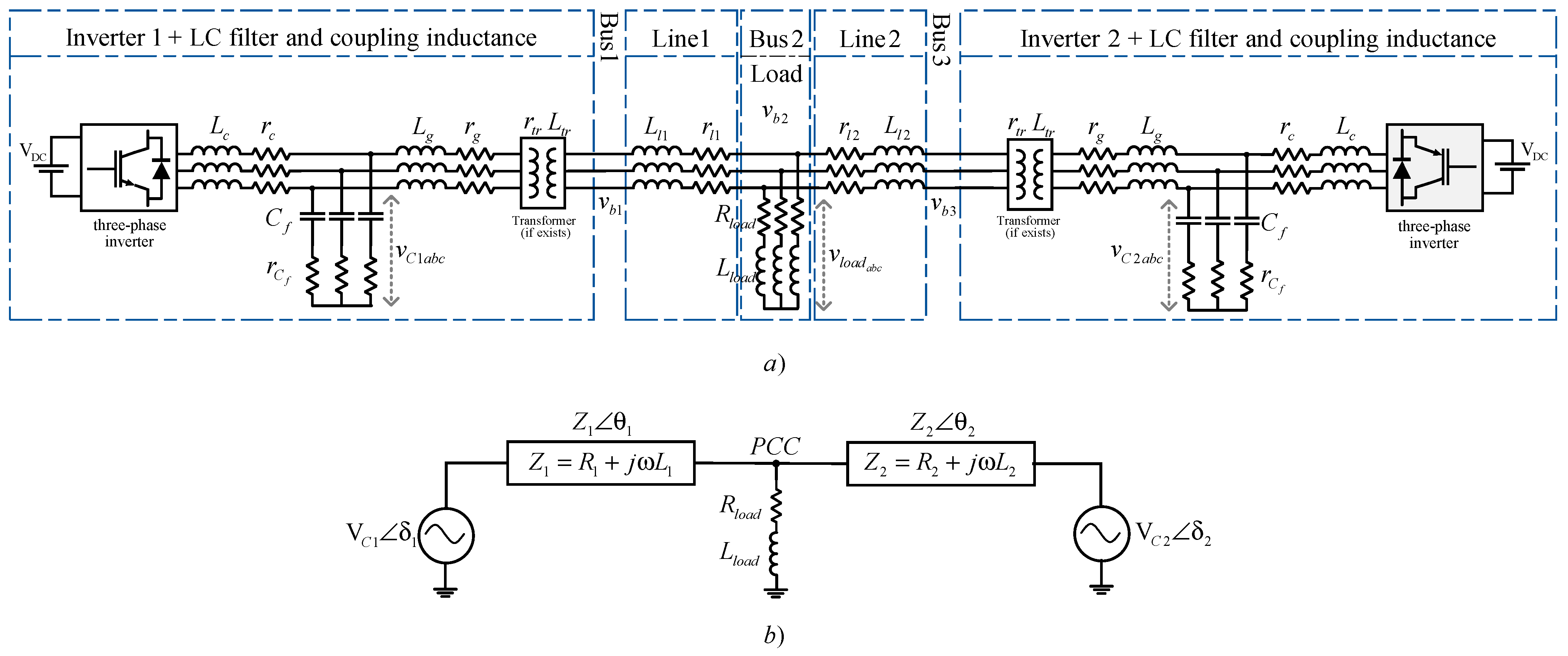
2. Control of Island Microgrids

Establishing a hierarchical control system for microgrids (MGs) is crucial for enhancing its efficiency, ensuring stability, and achieving an optimal closed-loop control system. The control system in MGs is typically divided into four levels: zero-level control, primary control, secondary control, and tertiary control [16,50,51]. Primary control focuses on local variables, such as frequency and voltage, and can be implemented in two ways, depending on the need for communication between parallel-connected grid-forming inverters (GFIs).

When droop control methods are applied locally to each GFI, communication is unnecessary, enabling autonomous operation. In terms of this mode, each GFI locally determines its reference voltage and frequency, which is a core principle of GFI operation in island MGs. These reference voltage and frequency values are then sent to the outer voltage controller and inner current controller to regulate the GFI’s output voltage and current [12,52]. In this paper, conventional droop control is adopted as the primary control method for autonomous power sharing between parallel-connected GFIs. Additionally, a virtual impedance scheme is adopted to enhance the performance of power sharing. PI voltage and PI current controllers are used as zero-level control methods to regulate the output voltage and current. The entire control system is implemented in regard to the dq-axis reference frame, which facilitates stability analysis of the MG. Secondary and tertiary control levels are beyond the scope of this paper.

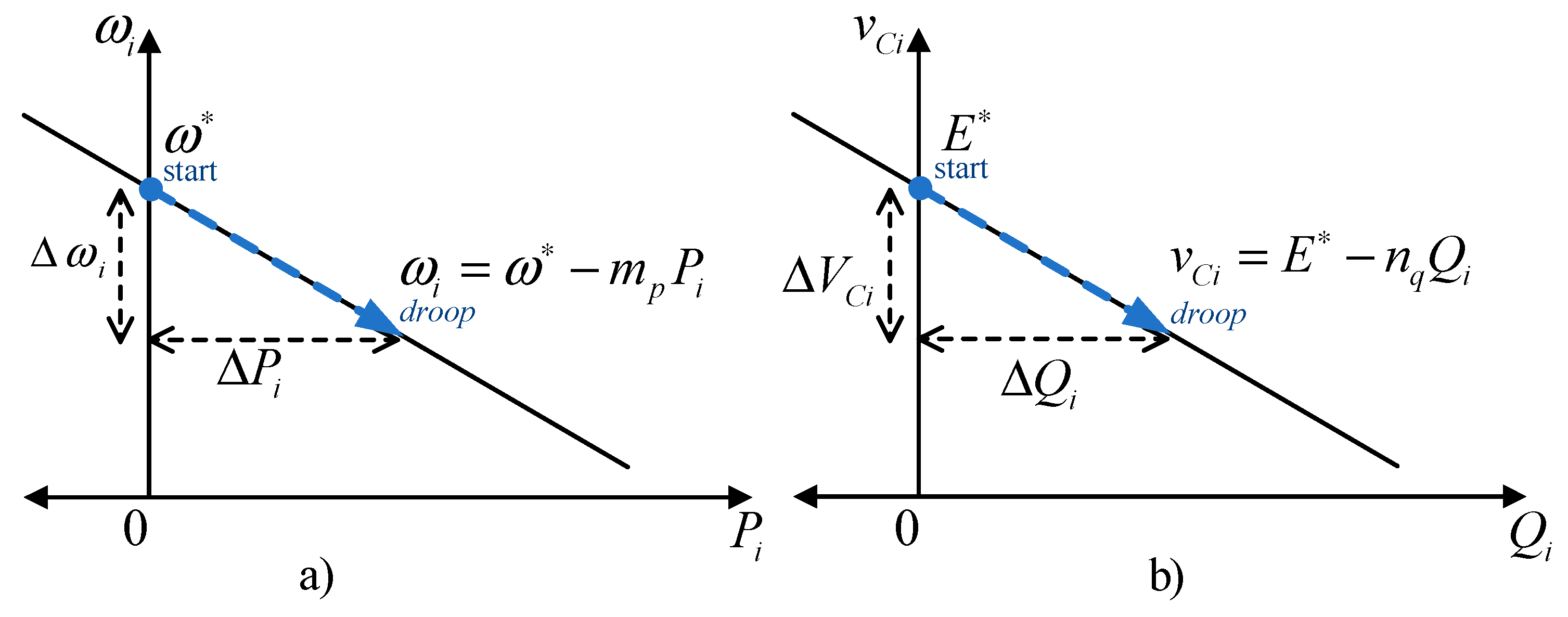
2.1. Power Sharing Based on Conventional Droop Control and Virtual Impedance

In island MGs, active and reactive powers must be shared correctly between the GFIs to ensure the stable operation of the MGs. In the literature, the droop control method is commonly applied in regard to MGs. The primary reason for adopting the droop control method is that it allows active and reactive power sharing between GFIs without the need for a communication network, i.e., autonomous operation. Figure 1a shows the typical structure of an island MG, including parallel-connected GFIs, and Figure 1b depicts the fundamental frequency equivalent of the MG, represented by ideal voltage sources at the fundamental frequency. The microgrid topology generally consists of a DC bus $V_{DC}$, an inverter, an LCL filter (and step-up transformer if present), lines, and loads.

In Figure 1b, $v_{\mathit{Ci}}=\sqrt{2}{V}_{Ci}\mathit{sin}\left({\omega }_{i}t+{\delta }_i\right)$ is the reference voltage for the ideal voltage source, ${\delta }_i$ is phase shifts of the sources with respect to $V_{load}\angle$0$°$. ${\omega }_i$ is the frequency in regard to rad/s for i.th GFI in MG. $V_{\mathit{load}}$ represents the load voltage at PCC. R_i and X_i are the total line resistance and reactance, respectively. The active power (P_i) and reactive power (Q_i) drawn from GFI_i ($i=1,2$) are given by Equations (1) and (2), respectively.

$$P_i={\displaystyle \frac{3}{{R_i}^2+{X_i}^2}}\left(R_i{V_{\mathit{Ci}}}^2-{R_i{V}_{\mathit{Ci}}V}_{\mathit{load}}\mathit{cos}{\delta }_i+V_{\mathit{Ci}}{V}_{\mathit{load}}{X}_i\mathit{sin}{\delta }_i\right),$$

(1)

$$Q_i={\displaystyle \frac{3}{{R_i}^2+{X_i}^2}}\left(X_i{V_{\mathit{Ci}}}^2-R_i{V}_i{V}_{\mathit{load}}\mathit{sin}{\delta }_i-{V_{\mathit{Ci}}V}_{\mathit{load}}{X}_i\mathit{cos}{\delta }_i\right).$$

(2)

Assuming that the line impedances are constant, the sensitivities of the active and reactive power to ${\delta }_i$ and $V_{\mathit{Ci}}$, respectively, are derived as shown in Equation (3).

$$\begin{array}{c}{\displaystyle \frac{d{P}_i}{d{\delta }_i}}={\displaystyle \frac{3\left(R_i{V}_{\mathit{Ci}}{V}_{\mathit{load}}\mathit{sin}{\delta }_i+V_{\mathit{Ci}}{V}_{\mathit{load}}{X}_i\mathit{cos}{\delta }_i\right)}{{R_i}^2+{X_i}^2}},\\ {\displaystyle \frac{d{P}_i}{d{V}_{\mathit{Ci}}}}={\displaystyle \frac{3\left(2R_i{V}_{\mathit{Ci}}-R_i{V}_{\mathit{load}}\mathit{cos}{\delta }_i+V_{\mathit{load}}{X}_i\mathit{sin}{\delta }_i\right)}{{R_i}^2+{X_i}^2}},\\ {\displaystyle \frac{d{Q}_i}{d{\delta }_i}}={\displaystyle \frac{3\left(-R_i{V}_{\mathit{Ci}}{V}_{\mathit{load}}\mathit{cos}{\delta }_i+V_{\mathit{Ci}}{V}_{\mathit{load}}{X}_i\mathit{sin}{\delta }_i\right)}{{R_i}^2+{X_i}^2}},\\ {\displaystyle \frac{d{Q}_i}{d{V}_{\mathit{Ci}}}}={\displaystyle \frac{3\left(2X_i{V}_{\mathit{Ci}}-R_i{V}_{\mathit{load}}\mathit{sin}{\delta }_i-V_{\mathit{load}}{X}_i\mathit{cos}{\delta }_i\right)}{{R_i}^2+{X_i}^2}}.\end{array}$$

(3)

Since the phase δ_i is quite small, $\mathit{sin}\left(\delta \right)\cong 0$ and $\mathit{cos}\left(\delta \right)\cong 1$ can be assumed. In this case, the sensitivities of the active and reactive power to ${\delta }_i$ and $V_{\mathit{Ci}}$, respectively, are as given by Equation (4). The output impedance of a GFI is not always purely resistive, inductive, or capacitive. In the case of a complex impedance, active and reactive powers cannot be controlled independently, as indicated in Equation (4). Therefore, in the literature, different types of droop control methods have been applied depending on whether the output impedance is resistive, inductive, or capacitive [21,24,53].

$$\begin{array}{c}{\displaystyle \frac{d{P}_i}{d{\delta }_i}}={\displaystyle \frac{3V_{\mathit{Ci}}{V}_{\mathit{load}}X}{{R_i}^2+{X_i}^2}},\\ {\displaystyle \frac{d{P}_i}{d{V}_{\mathit{Ci}}}}={\displaystyle \frac{3\left(2R_i{V}_{\mathit{Ci}}-R_i{V}_{\mathit{load}}\right)}{{R_i}^2+{X_i}^2}},\\ {\displaystyle \frac{d{Q}_i}{d{\delta }_i}}={\displaystyle \frac{-3R_i{V}_{\mathit{Ci}}{V}_{\mathit{load}}}{{R_i}^2+{X_i}^2}},\\ {\displaystyle \frac{d{Q}_i}{d{V}_{\mathit{Ci}}}}={\displaystyle \frac{3\left(2X_i{V}_{\mathit{Ci}}-V_{\mathit{load}}{X}_i\right)}{{R_i}^2+{X_i}^2}}.\end{array}$$

(4)

In this paper, an inductive output impedance is considered since the coupling inductance, transformer leakage inductance, and line inductance cause the output impedance of the GFI to be highly inductive. Consequently, the sensitivities of the active and reactive power are derived from Equation (5).

$$\begin{array}{c}{\displaystyle \frac{d{P}_i}{d{\delta }_i}}={\displaystyle \frac{3V_{\mathit{Ci}}{V}_{\mathit{lod}}}{X_i}},\\ {\displaystyle \frac{d{P}_i}{d{V}_{\mathit{Ci}}}}=0,\\ {\displaystyle \frac{d{Q}_i}{d{\delta }_i}}=0,\\ {\displaystyle \frac{dQ}{d{V}_{\mathit{Ci}}}}={\displaystyle \frac{3\left(2V_{\mathit{Ci}}-V_{\mathit{load}}\right)}{X_i}}.\end{array}$$

(5)

Based on Equation (5), the droop control method is applied according to the relationship between $P~\omega$ and $Q~V_C$, which allows for the independent control of the active and reactive power. The conventional droop control equations are given by Equation (6). In Equation (6) [4], ${\omega }_i$ and $V_{Ci}$ are the i.th GFI angular frequency in regard to rad/s and the voltage magnitude, ${\omega }^{\ast }$ and $E^{\ast }$ are the reference angular frequency and reference voltage magnitude, and m_p and n_q are the active power droop coefficient and reactive power droop coefficient, respectively.

$$\begin{array}{c}{\omega }_i={\omega }^{\ast }-m_p{P}_i,\\ V_{\mathit{Ci}}=E^{\ast }-n_q{Q}_i.\end{array}$$

(6)

A graphical representation of conventional droop control is shown in Figure 2. The droop control method is widely used for accurate power sharing in regard to parallel-connected GFIs. However, its transient and steady-state performance is highly sensitive to variations or mismatches in line impedance, as well as external disturbances. One significant issue that arises from these differences is the occurrence of circulating currents between GFIs, caused by discrepancies in their output voltages and parameter variations. These circulating currents can lead to overcurrent problems, potentially disrupting the parallel operation of GFIs. To address these challenges, it is common practice in the literature to implement a virtual impedance scheme, which helps mitigate these drawbacks [24,54].

2.2. Cascaded Outer Voltage and Inner Current Control of Island Microgrid

In island MG applications, GFIs typically consist of a voltage source inverter (VSI) with an LC output filter, as depicted in Figure 3. The implementation of zero-level control in regard to GFIs is vital for achieving the desired control objectives, such as zero steady-state error, disturbance rejection, harmonic compensation, and preventing interactions between the control loops. In regard to the control system, a cascaded outer voltage controller and inner current controller, along with FF control and virtual impedance, are adopted to control the state variables, namely the capacitor voltage $v_C$ for the voltage controller, and the converter-side filter current $i_c$ for the current controller. The droop control sets the reference capacitor voltage $v_{\mathit{Cref}}$ and the frequency ω_i of the GFI for the outer voltage control loop, whereas the outer voltage control loop provides the reference filter current $i_{\mathit{cref}}$ for the inner current control loop.

Additionally, a virtual impedance scheme is integrated into the system to improve both the transient and steady-state performance, while feed-forward (FF) control is incorporated to enhance disturbance rejection, as illustrated in Figure 3. Closed-loop control in microgrids (MGs) can be implemented in regard to three different reference frames: the abc-axis stationary reference frame, the αβ-axes stationary reference frame using Clarke transformation, and the dq-axis synchronous reference frame using Park transformation [51]. Each reference frame utilizes specific controllers to achieve closed-loop control of the GFIs. For example, proportional–integral (PI) controllers are typically used in regard to the dq-axis, while proportional–resonant (PR) controllers are applied in regard to the αβ-axes.

The PI controller offers superior performance when controlling DC signals compared to a PR controller, particularly in terms of reference tracking, zero steady-state error, and disturbance rejection [55,56]. In regard to synchronous reference frame control, three-phase AC signals are transformed into DC signals using the Park transformation, where the angular frequency, ω, rotates synchronously. This transformation enables the application of the PI controller in regard to the dq-axis. However, due to the nature of the Park transformation, cross-coupling terms arise between the d- and q-axes. Decoupling these terms is essential to independently control the d- and q-axis variables. Consequently, as illustrated in Figure 3, which presents the overall control block diagram of a GFI, a decoupling scheme is integrated into the control algorithm for both the voltage and current controllers. The detailed implementation of this scheme is further elaborated in Figure 7.

Proper tuning of the outer PI voltage controller and the inner PI current controller is crucial for cascaded controller design, as it directly impacts the system’s performance and stability. The controller gains determine the dynamic response of both the outer and inner control loops. To ensure optimal performance, the inner current control loop must operate significantly faster than the outer voltage control loop, meaning that the bandwidth of the inner current loop should be substantially wider than that of the outer voltage loop. This ensures minimal interaction between the control loops, allowing for more efficient and stable operation. In this paper, the inner current loop bandwidth is set to 1 kHz, while the outer voltage control loop bandwidth is set to 175 Hz.

In the classical PI controller design approach in regard to the dq-axis, the cross-coupling terms are often omitted by assuming that the decoupling scheme effectively eliminates these terms. Based on this assumption, the control loop can be modeled as a single-input, single-output (SISO) transfer function. A common method for tuning the bandwidths of the outer voltage and inner current control loops is the zero-pole cancellation approach. Furthermore, special attention must be paid to the inner current control loop, as time delays introduced by digital control can reduce its achievable bandwidth. This reduction in bandwidth can lead to interactions with the outer voltage control loop if the system is not properly designed. Additionally, time delays can negatively affect the performance of both the decoupling scheme and feed-forward (FF) control [57], which may disable the assumption about the linearity of the overall system. One of the contributions of this paper lies in the accurate derivation of outer voltage and inner current control small-signal models for the purpose of stability analysis. In contrast to conventional small-signal modeling, this study incorporates the angular frequency, ω, as a state variable during the modeling of the voltage and current controllers, subsequently including it in the derived small-signal model. This approach allows for more accurate stability analysis of MGs by directly accounting for the impact of frequency variations on the controller dynamics. Section 3 addresses the effects of the time delay and the corresponding modeling approach.

3. Time Delay Representation in Regard to the dq-Axis for Use in Small-Signal Stability Analysis [46,47]

A time delay was first incorporated into the small-signal stability analysis in regard to the dq-axis by [46,47]. In the referenced studies, a time delay was typically incorporated directly into the dq-axis to obtain a small-signal model. However, this approach neglects the phase shift introduced by the time delay in regard to the abc-axis. The motivation of this paper lies in representing a time delay in regard to the abc-axis and incorporating the phase shift into the dq-axis for more accurate small-signal modeling. The conventional approach to modeling a time delay in regard to the dq-axis involves using an equivalent transfer function, derived through the use of the Padé approximation, as shown in

Table 2. Padé approximation transfer functions of time delay.

Order	$\mathbf{Transfer} \mathbf{Function}—\mathit{T}{\mathit{F}}_{{\mathit{T}}_{\mathit{td}}}\left(\mathbf{s}\right)$
1	${\displaystyle \frac{2-T_{\mathit{td}}s}{2+T_{\mathit{td}}s}}$
2	${\displaystyle \frac{12-6T_{\mathit{td}}s+T_{\mathit{td}}^2{s}^2}{12+6T_{\mathit{td}}s+T_{\mathit{td}}^2{s}^2}}$
3	${\displaystyle \frac{120-60T_{\mathit{td}}s+12T_{\mathit{td}}^2{s}^2-T_{\mathit{td}}^3{s}^3}{120+60T_{\mathit{td}}s+12T_{\mathit{td}}^2{s}^2+T_{\mathit{td}}^3{s}^3}}$
4	${\displaystyle \frac{1680-840T_{\mathit{td}}s+180T_{\mathit{td}}^2{s}^2-20T_{\mathit{td}}^3{s}^3+T_{\mathit{td}}^4{s}^4}{1680+840T_{\mathit{td}}s+180T_{\mathit{td}}^2{s}^2+20T_{\mathit{td}}^3{s}^3+T_{\mathit{td}}^4{s}^4}}$

. However, the conventional approach assumes that digital control-induced time delays occur in regard to the dq-axis. This assumption does not accurately reflect how digital control systems operate, wherein a time delay naturally occurs in regard to the abc-axis. As a result, the conventional approach presented in [46,47] does not accurately represent digital control-induced time delays in regard to the dq-axis, as demonstrated in Figure 4. Figure 4a,b provides a comparison between the conventional approach and the proposed accurate time delay representation in regard to the dq-axis synchronous reference frame. In Figure 4, v_md, v_mq, and T_td are the d-axis and q-axis modulation signal and time delay in seconds, respectively.

3.1. Necessity of Modeling the Time Delay

The presence of a time delay can cause a phase lag that reduces the phase margin (PM) and bandwidth of the current control loop. In other words, it causes complex roots to move towards the right half-plane. In this case, the inner current control loop may also interfere with the outer loops, i.e., the voltage control loop and the droop control, which have slower dynamics [58]. This interference has a negative impact on the overall performance of the system, and if the inner current control loop is not designed considering digital control-induced time delays, it can lead to instability and a significant decline in the system performance. It is, therefore, crucial to design the current control loop, where a time delay occurs, in order to maintain the desired performance and stability of the system. As a result, to ensure proper controller design, it is necessary to model the time delay for use in stability analysis, so that the time delay’s effect on stability may be assessed through small-signal analysis.

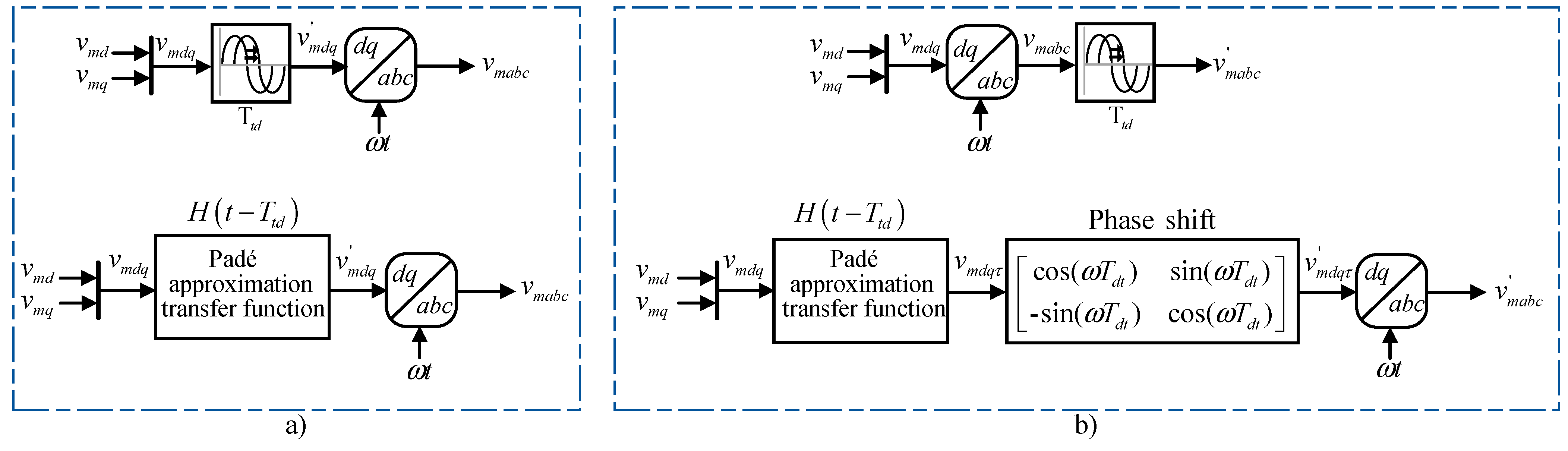
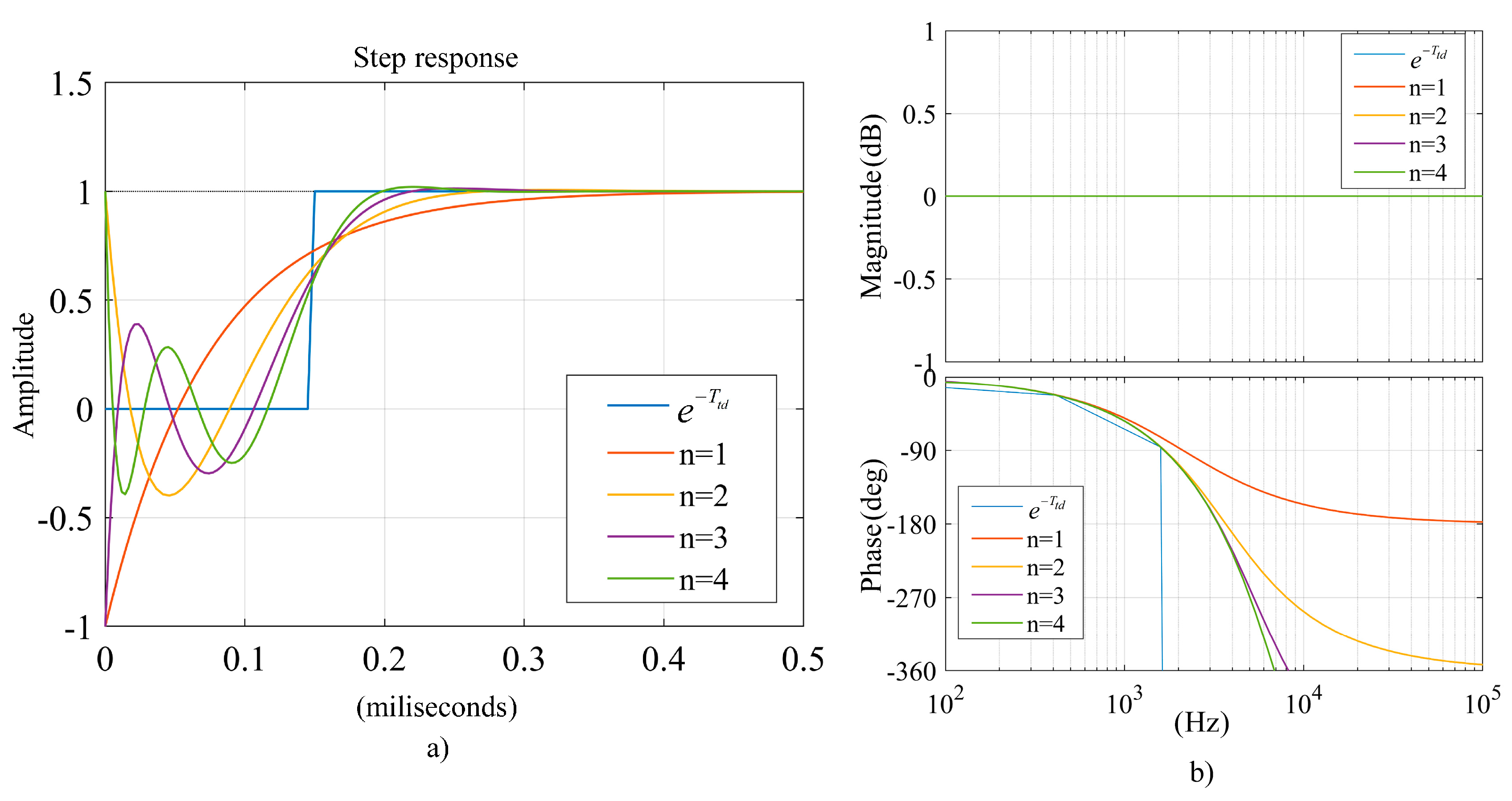
3.2. Conventional Time Delay Modeling Approach

In digital control systems, a time delay occurs in two ways: the first arises from a digital computational delay and the second is due to a pulse-width modulation (PWM) delay. A digital computational delay is related to the sampling time T_samp and treated as a zero-order hold (ZOH) action. It appears in two ways depending on the sampling method: (1) single update PWM and (2) double update PWM. In regard to single update PWM, the sampling frequency is equal to the switching frequency, whereas in regard to double update PWM, the sampling frequency is twice the switching frequency. In this paper, the double update PWM method is employed; therefore, the digital computational delay is chosen as 0.5T_samp, which is widely accepted as the average value. On the other hand, a PWM delay is related to the microcontroller PWM generation algorithm. The microcontroller PWM unit generates switching signals after a one-cycle delay (T_samp), which is treated as a transport delay [46,47]. As a result, the total time delay is 1.5T_samp, which is the sum of the computational delay (0.5T_samp) and the PWM delay (T_samp).

In this paper, the switching frequency is f_sw = 5 kHz, leading to a total time delay of T_td = 1.5/f_sw. As a common approach, the total time delay is modelled using an exponential function T_td(s) = $e^{-s{T}_{td}}$. To incorporate this model into a closed loop system as a transfer function, the Padé approximation is commonly employed in regard to the conventional time delay modeling approach, as given in Table 2 for different orders. However, this approach neglects the phase shift effect introduced by a time delay in regard to the abc-axis, which can significantly impact system stability.

In Figure 5, the step response and frequency responses of the Padé approximation transfer functions given in Table 2 are shown for a total time delay of T_td = 1.5/f_sw. A crucial aspect of employing Padé approximations is the selection of the appropriate approximation order. This choice involves a fundamental trade-off between the accuracy and the computational complexity introduced by the approximation order. Simply, there are two phenomena to consider when selecting the approximation order: (1) the phase response, and (2) the non-minimum phase effect. In Figure 5b, it can easily be seen that the ideal time delay phase response decreases linearly with the frequency (blue line). As the order increases, the phase response gets closer to the ideal time delay phase response at higher frequencies. For n = 1 (orange line) and n = 2 (yellow line), the phase response significantly differs from the ideal time delay phase response. On the other hand, for n = 3 (magenta line) and n = 4 (green line), the phase response is much closer to the ideal one. From this point on, increasing the approximation order makes no significant difference. The primary drawback of using higher-order Padé approximations is the increase in computational complexity. As a result, the choice of the 4th-order approximation is based on achieving a reasonable trade-off between accuracy and computational complexity. Using the Padé approximation also introduces a non-minimum phase (right-half plane zero), as can be seen from the step response in Figure 5a and the transfer functions in Table 2. This effect is significant especially in terms of the first-order approximation, which dips significantly below zero before changing direction. This effect can be reduced by using higher-order approximation, which more closely matches the ideal system response. As a result, the choice of a 4th-order approximation is reasonable and consistent with the step and frequency response results for a time delay of T_td = 150 μs.

3.3. Proposed Accurate Time Delay Representation in Regard to the dq-Axis

3.3.1. Time Delay in Regard to the abc-Axis Stationary Reference Frame

In a control system, to generate the modulation signal, v_mabc, the dq-axis reference voltage produced by the inner current controller is initially transformed into a stationary reference frame (αβ-axis or abc-axis) using the angular frequency, θ = ωt, as illustrated in Figure 4b. Then, modulation signal v_mabc is subjected to a time delay due to discretization and pulse-width modulation (PWM) actions in regard to the microcontroller, as discussed in Section 3.1. Finally, PWM switching is applied to the power switches, so that the converter-side reference voltage is obtained. As a result, a time delay occurs in regard to the stationary reference frame, which manifests as a phase shift in the sinusoidal waveform, as illustrated in Figure 4b. To derive the equivalent of the time delay model $e^{-s{T}_{\mathit{td}}}$ in regard to the stationary frame, the delayed output function Y(s) with a sinusoidal input represented by $K_{in}\omega /(s^2+{\omega }^2)$ is considered, as in Equation (7), where K is the input gain and $\omega$ is the angular frequency.

$$Y(s)={\displaystyle \frac{K_{in}\omega }{s^2+{\omega }^2}}{e}^{-s{T}_{\mathit{td}}}.$$

(7)

Applying the inverse Laplace transform in regard to Equation (7) yields Equation (8), where $H\left(t-T_{td}\right)$ is the Heaviside function and $-\omega T_{\mathit{td}}$ is the phase shift.

$$y\left(t)=K_{in}H\right(t-T_{\mathit{td}})\mathit{sin}\left(\omega t-\omega T_{\mathit{td}}\right).$$

(8)

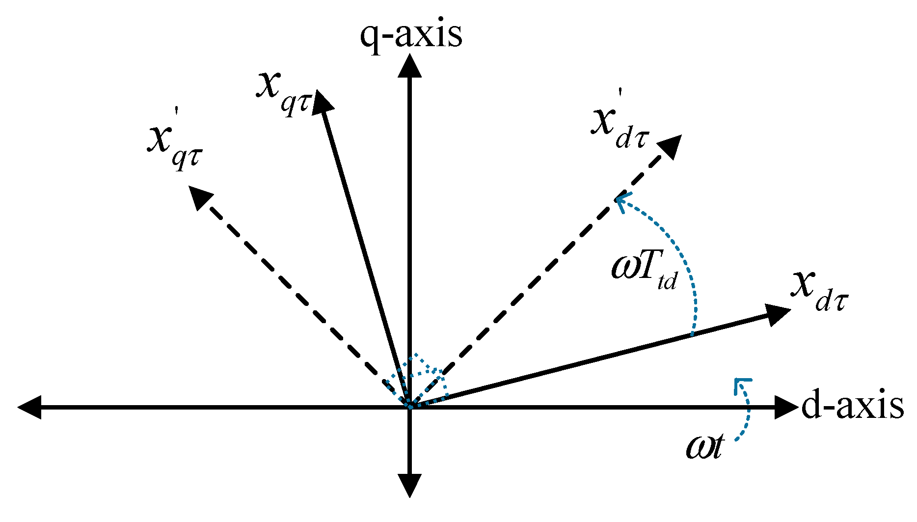
3.3.2. Accurate Time Delay Representation in Regard to the dq-Axis

From Equation (8), it is clearly observed that when the input is a sinusoidal waveform, the time response of the system has a phase shift $-\omega T_{\mathit{td}}$, along with a time dependent amplitude H(t−T_td). However, the conventional approach to modeling a time delay in regard to the dq-axis bypasses the phase shift ($-\omega T_{\mathit{td}}$). Instead, it approximates the Heaviside function H(t−T_td) exclusively using the Padé approximation, as given in Table 2. This paper proposes an accurate representation of the time delay in regard to the dq-axis as a novelty by incorporating not only the Heaviside function H(t−T_td), but also the phase shift $-\omega T_{\mathit{td}}$, as they significantly affect the stability of island MGs.

The first step (the conventional approach, [46,47]): In this paper, a 4th-order Padé approximation transfer function is employed to represent the time delay more accurately. Based on the proposed accurate time delay representation in regard to the dq-axis depicted in Figure 4b, a small-signal model of the time delay for T_td = 150 μs is derived in two steps. The first step involves deriving the small-signal model of the 4th-order Padé approximation as provided in Table 2 and in Equation (9).

$$T{F}_{T_{\mathit{td}}}(s)={\displaystyle \frac{K-L{T}_{\mathit{td}}s+M{T}_{\mathit{td}}^2{s}^2-N{T}_{\mathit{td}}^3{s}^3+T_{\mathit{td}}^4{s}^4}{K+L{T}_{\mathit{td}}s+M{T}_{\mathit{td}}^2{s}^2+N{T}_{\mathit{td}}^3{s}^3+T_{\mathit{td}}^4{s}^4}},$$

(9)

where K = 1680, L = 840, M = 180, and N = 20. A state-space model with the fictitious state variables, ${\tau }_{dk}$ and ${\tau }_{qk}$, where k = 1, 2, 3, 4 for the 4th-order Padé approximation transfer function is given in Equation (10).

$$\begin{array}{ll}\begin{array}{l}{\displaystyle \frac{d{\tau }_{d1}}{\mathit{dt}}}={\tau }_{d2},\\ {\displaystyle \frac{d{\tau }_{d2}}{\mathit{dt}}}={\tau }_{d3},\\ {\displaystyle \frac{d{\tau }_{d3}}{\mathit{dt}}}={\tau }_{d4},\\ {\displaystyle \frac{d{\tau }_{d4}}{\mathit{dt}}}=-N{\tau }_{d1}-M{\tau }_{d2}-L{\tau }_{d3}-K{\tau }_{d4},\end{array}& \begin{array}{l}{\displaystyle \frac{d{\tau }_{q1}}{\mathit{dt}}}={\tau }_{q2},\\ {\displaystyle \frac{d{\tau }_{q2}}{\mathit{dt}}}={\tau }_{q3},\\ {\displaystyle \frac{d{\tau }_{q3}}{\mathit{dt}}}={\tau }_{q4},\\ {\displaystyle \frac{d{\tau }_{q4}}{\mathit{dt}}}=-N{\tau }_{q1}-M{\tau }_{q2}-L{\tau }_{q3}-K{\tau }_{q4}.\end{array}\end{array}$$

(10)

The output of the Padé approximation transfer function $v_{md\tau }$ and $v_{mq\tau }$ are specified in Equation (11).

$$\begin{array}{c}{v}_{\mathit{md}\tau }=-2M{\tau }_{d2}-2K{\tau }_{d4}-v_{\mathit{md}},\\ v_{\mathit{mq}\tau }=-2M{\tau }_{q2}-2K{\tau }_{q4}-v_{\mathit{mq}}.\end{array}$$

(11)

If the linearization process is applied to the state-space model of the 4th-order Padé approximation transfer function, the resulting equation is given in Equation (12). In Equation (12), ∆ before the state variables represents the linearized equivalent of the state variables, and the dot over the ∆ represents a derivative of the state variables.

$$\begin{array}{ll}\begin{array}{l}\dot{\mathsf{\Delta }}{\tau }_{d1}=\mathsf{\Delta }{\tau }_{d2},\\ \dot{\mathsf{\Delta }}{\tau }_{d2}=\mathsf{\Delta }{\tau }_{d3},\\ \dot{\mathsf{\Delta }}{\tau }_{d3}=\mathsf{\Delta }{\tau }_{d4},\\ \dot{\mathsf{\Delta }}{\tau }_{d4}=-N\mathsf{\Delta }{\tau }_{d1}-M\mathsf{\Delta }{\tau }_{d2}-L\mathsf{\Delta }{\tau }_{d3}-K\mathsf{\Delta }{\tau }_{d4},\\ \mathsf{\Delta }{v}_{\mathit{md}\tau }=-2M\mathsf{\Delta }{\tau }_{d2}-2K\mathsf{\Delta }{\tau }_{d4}-\mathsf{\Delta }{v}_{\mathit{md}},\end{array}\hspace{1em}\hspace{1em}& \begin{array}{l}\dot{\mathsf{\Delta }}{\tau }_{q1}=\mathsf{\Delta }{\tau }_{q2},\\ \dot{\mathsf{\Delta }}{\tau }_{q2}=\mathsf{\Delta }{\tau }_{q3},\\ \dot{\mathsf{\Delta }}{\tau }_{q3}=\mathsf{\Delta }{\tau }_{q4},\\ \dot{\mathsf{\Delta }}{\tau }_{q4}=-\mathsf{\Delta }N{\tau }_{q1}-\mathsf{\Delta }M{\tau }_{q2}-\mathsf{\Delta }L{\tau }_{q3}-\mathsf{\Delta }K{\tau }_{q4},\\ \mathsf{\Delta }{v}_{\mathit{mq}\tau }=-2M\mathsf{\Delta }{\tau }_{q2}-2K\mathsf{\Delta }{\tau }_{q4}-\mathsf{\Delta }{v}_{\mathit{mq}}.\end{array}\end{array}$$

(12)

If Equation (12) is arranged in matrix form, then the state-space model of the 4th-order Padé approximation is obtained, as in Equation (13a):

$$\begin{array}{c}\left[\begin{array}{c}\dot{\mathsf{\Delta }}{\tau }_{\mathit{dk}}\\ \dot{\mathsf{\Delta }}{\tau }_{\mathit{qk}}\end{array}\right]=A_{\tau }\left[\begin{array}{c}\mathsf{\Delta }{\tau }_{\mathit{dk}}\\ \mathsf{\Delta }{\tau }_{\mathit{qk}}\end{array}\right]+B_{\tau }\left[\begin{array}{c}\mathsf{\Delta }{v}_{\mathit{md}}\\ \mathsf{\Delta }{v}_{\mathit{mq}}\end{array}\right], \\ \left[\begin{array}{c}\mathsf{\Delta }{v}_{\mathit{md}\tau }\\ \mathsf{\Delta }{v}_{\mathit{mq}\tau }\end{array}\right]=C_{\tau }\left[\begin{array}{c}\mathsf{\Delta }{\tau }_{\mathit{dk}}\\ \mathsf{\Delta }{\tau }_{\mathit{qk}}\end{array}\right]+D_{\tau }\left[\begin{array}{c}\mathsf{\Delta }{v}_{\mathit{md}}\\ \mathsf{\Delta }{v}_{\mathit{mq}}\end{array}\right].\end{array}$$

(13a)

The A_τ, B_τ, C_τ, and D_τ matrices in Equation (13a) are given below in Equation (13b):

$$\begin{gathered} A_{\tau }=\left[\begin{array}{cc}\begin{array}{cccc}0& 1& 0& 0\\ 0& 0& 1& 0\\ 0& 0& 0& 1\\ -N& -M& -L& -K\end{array}& {\left[0\right]}_{4 \times 4}\\ {\left[0\right]}_{4 \times 4}& \begin{array}{cccc}0& 1& 0& 0\\ 0& 0& 1& 0\\ 0& 0& 0& 1\\ -N& -M& -L& -K\end{array}\end{array}\right], B_{\tau }={\left[\begin{array}{cccccccc}0& 0& 0& 1& 0& 0& 0& 0\\ 0& 0& 0& 0& 0& 0& 0& 1\end{array}\right]}^T, \\ {C}_{\tau }=\left[\begin{array}{cccccccc}0& 2M& 0& -2K& 0& 0& 0& 0\\ 0& 0& 0& 0& 0& -2M& 0& -2K\end{array}\right], D_{\tau }=\left[\begin{array}{cc}1& 0\\ 0& 1\end{array}\right]. \end{gathered}$$

(13b)

The second step: This step involves deriving small-signal representation of the phase shift presented in Equation (8). To develop a more precise time delay representation in regard to the dq-axis, it is essential to address the phase shift $-\omega T_{\mathit{td}}$ in two ways. Firstly, instead of using $\omega t$ as shown in Figure 4a, reference frame transformation can be applied using $\left(\omega t-\omega T_{\mathit{td}}\right)$. However, in this way, it is impossible to develop a small-signal model in dq-axis rotating with $\omega t$. Secondly, a dq-axes equivalent model of the phase shift $-\omega T_{\mathit{td}}$ should be introduced, allowing reference frame transformation to be performed using ωt. In Figure 6, dq-axis representation of the phase shift, $-\omega T_{\mathit{td}}$, is illustrated. This approach results in a model that is fully based on dq-axis rotation with $\omega t$, facilitating development of a small-signal model for the entire system. This method represents the novelty of this paper.

A three-phase variable can be converted into the dq-axis using the transformation $x=\left|X\right|e^{j\theta }={\left|X\right|}_{d\tau }+j{\left|X\right|}_{q\tau }$, where x represents a three-phase variable, x_dτ is the d-axis component, x_qτ is the q-axis component, $\left|X\right|$ represents the magnitude of the variable, and θ represents the angular frequency. If θ = ωt, x_dτ = v_mdτ and x_qτ = v_mqτ, then the output of the Padé approximation transfer function v_mdτ and v_mqτ are obtained, as shown in Equation (14).

$$\begin{array}{c}{v}_{\mathit{md}\tau }=\left|v_{\mathit{md}\tau }\right|\mathit{cos}\left(\omega t\right),\\ v_{\mathit{mq}\tau }=\left|v_{\mathit{mq}\tau }\right|\mathit{sin}\left(\omega t\right).\end{array}$$

(14)

For θ = ωt − ωT_td, the output of the phase shift in regard to dq-axis $v_{\mathit{md}\tau }^{\prime }$ and $v_{\mathit{mq}\tau }^{\prime }$ are obtained as in Equation (15).

$$\begin{array}{c}{v}_{\mathit{md}\tau }^{\prime }=\left|v_{\mathit{md}\tau }\right|\mathit{cos}\left(\omega t-\omega T_{\mathit{td}}\right),\\ v_{\mathit{mq}\tau }^{\prime }=\left|v_{\mathit{mq}\tau }\right|\mathit{sin}\left(\omega t-\omega T_{\mathit{td}}\right).\end{array}$$

(15)

Equation (15) can be expressed using an open form of the trigonometric functions with the phase shift, $-\omega T_{\mathit{td}}$, as shown in Equation (16).

$$\begin{array}{c}{v}_{\mathit{md}\tau }^{\prime }=\left|v_{\mathit{md}\tau }\right|\left[\mathit{cos}\left(\omega t\right)\mathit{cos}\left(-\omega T_{\mathit{td}}\right)+\mathit{sin}\left(\omega t\right)\mathit{sin}\left(-\omega T_{\mathit{td}}\right)\right],\\ v_{\mathit{mq}\tau }^{\prime }=\left|v_{\mathit{mq}\tau }\right|\left[\mathit{sin}\left(\omega t\right)\mathit{cos}\left(-\omega T_{\mathit{td}}\right)-\mathit{cos}\left(\omega t\right)\mathit{sin}\left(-\omega T_{\mathit{td}}\right)\right].\end{array}$$

(16)

Putting the output of the Padé approximation transfer function v_mdτ and v_mqτ into Equation (16) and rearranging it in terms of a matrix form yields Equation (17), which represents the equivalent model of the phase shift $-\omega T_{\mathit{td}}$ in regard to the dq-axis. This model allows reference frame transformations to be performed using $\omega t$, rather than $\left(\omega t-\omega T_{\mathit{td}}\right)$, as described above.

$$\left[\begin{array}{c}{v}_{\mathit{md}\tau }^{\prime }\\ v_{\mathit{mq}\tau }^{\prime }\end{array}\right]=\left[\begin{array}{cc}\mathit{cos}\left(\omega T_{\mathit{td}}\right)& \mathit{sin}\left(\omega T_{\mathit{td}}\right)\\ -\mathit{sin}\left(\omega T_{\mathit{td}}\right)& \mathit{cos}\left(\omega T_{\mathit{td}}\right)\end{array}\right]\left[\begin{array}{c}{v}_{\mathit{md}\tau }\\ v_{\mathit{mq}\tau }\end{array}\right].$$

(17)

By applying linearization to the phase shift in Equation (17) with respect to the state variables v_mdτ, v_mqτ, and ω, the following small-signal model is derived, as shown in Equation (18):

$$\begin{array}{l}\mathsf{\Delta }{v}_{\mathit{md}\tau }^{\prime }=cos\left({\omega }_o{T}_{\mathit{td}}\right)\mathsf{\Delta }{v}_{\mathit{md}\tau }+sin\left({\omega }_o{T}_{\mathit{td}}\right)\mathsf{\Delta }{v}_{\mathit{mq}\tau }+\left(-V_{\mathit{md}\tau }{T}_{\mathit{td}}\mathit{sin}\left({\omega }_o{T}_{\mathit{td}}\right)+V_{\mathit{mq}\tau }{T}_{\mathit{td}}\mathit{cos}\left({\omega }_o{T}_{\mathit{td}}\right)\right)\mathsf{\Delta }\omega ,\\ \mathsf{\Delta }{v}_{\mathit{mq}\tau }^{\prime }=-sin\left({\omega }_o{T}_{\mathit{td}}\right)\mathsf{\Delta }{v}_{\mathit{md}\tau }+cos\left({\omega }_o{T}_{\mathit{td}}\right)\mathsf{\Delta }{v}_{\mathit{mq}\tau }+\left(-V_{\mathit{md}\tau }{T}_{\mathit{td}}\mathit{cos}\left({\omega }_o{T}_{\mathit{td}}\right)-V_{\mathit{mq}\tau }{T}_{\mathit{td}}\mathit{sin}\left({\omega }_o{T}_{\mathit{td}}\right)\right)\mathsf{\Delta }\omega ,\end{array}$$

(18)

where V_mdτ, V_mqτ, and ω_o are the operating point values for the d-axis input in terms of the phase shift, the q-axis input in terms of the phase shift, and the angular frequency, respectively. Equation (18) can be rewritten in matrix form, as given in Equation (19a).

$$\left[\begin{array}{c}\mathsf{\Delta }{v}_{\mathit{md}\tau }^{\prime }\\ \mathsf{\Delta }{v}_{\mathit{mq}\tau }^{\prime }\end{array}\right]=E_{\tau }\left[\begin{array}{c}\mathsf{\Delta }{v}_{\mathit{md}\tau }\\ \mathsf{\Delta }{v}_{\mathit{mq}\tau }\end{array}\right]+F_{\tau }\left[\mathsf{\Delta }\omega \right].$$

(19a)

The E_τ and F_τ matrices in Equation (19a) are given below in Equation (19b).

$$E_{\tau }=\left[\begin{array}{cc}\mathit{cos}\left({\omega }_o{T}_{\mathit{td}}\right)& \mathit{sin}({\omega }_o{T}_{\mathit{td}})\\ -\mathit{sin}({\omega }_o{T}_{\mathit{td}})& \mathit{cos}({\omega }_o{T}_{\mathit{td}})\end{array}\right], F_{\tau }=\left[\begin{array}{c}-V_{\mathit{md}\tau }{T}_{\mathit{td}}\mathit{sin}\left({\omega }_o{T}_{\mathit{td}}\right)+V_{\mathit{mq}\tau }{T}_{\mathit{td}}\mathit{cos}\left({\omega }_o{T}_{\mathit{td}}\right)\\ -V_{\mathit{md}\tau }{T}_{\mathit{td}}\mathit{cos}\left({\omega }_o{T}_{\mathit{td}}\right)-V_{\mathit{mq}\tau }{T}_{\mathit{td}}\mathit{sin}\left({\omega }_o{T}_{\mathit{td}}\right)\end{array}\right].$$

(19b)

Consequently, the proposed accurate time delay small-signal model is provided in Equation (20). This model is uniquely designed for small-signal stability analysis, presenting a precise method for accurate representation of a time delay in regard to the dq-axis.

$$\begin{array}{l}\left[\begin{array}{c}\dot{\mathsf{\Delta }}{\tau }_{dk}\\ \dot{\mathsf{\Delta }}{\tau }_{qk}\end{array}\right]=A_{\tau }\left[\begin{array}{c}\mathsf{\Delta }{\tau }_{dk}\\ \mathsf{\Delta }{\tau }_{qk}\end{array}\right]+B_{\tau }\left[\begin{array}{c}\mathsf{\Delta }{v}_{\mathit{md}}\\ \mathsf{\Delta }{v}_{\mathit{mq}}\end{array}\right],\\ \left[\begin{array}{c}\mathsf{\Delta }{v}_{\mathit{md}\tau }^{\prime }\\ \mathsf{\Delta }{v}_{\mathit{mq}\tau }^{\prime }\end{array}\right]=E_{\tau }{C}_{\tau }\left[\begin{array}{c}\mathsf{\Delta }{\tau }_{dk}\\ \mathsf{\Delta }{\tau }_{qk}\end{array}\right]+E_{\tau }{D}_{\tau }\left[\begin{array}{c}\mathsf{\Delta }{v}_{\mathit{md}}\\ \mathsf{\Delta }{v}_{\mathit{mq}}\end{array}\right]+F_{\tau }\left[\mathsf{\Delta }\omega \right].\end{array}$$

(20)

It is important to note that computational load introduced by the conventional time delay modeling is only due to the order of the Padé approximation. A n.th-order Padé approximation results in a rational transfer function, wherein both the numerator and denominator are n.th order polynomials. This increases the order of the transfer function and directly translates into a higher number of poles and zeros in the system model, and consequently, a larger number of states in regard to its state-space representation. In the dq-axis, the n.th order state-space model results in a state-space model with twice the number of state variables. Thus, higher-order Padé approximation increases the system’s matrix size, which means that the number of eigenvalues in the stability analysis is also increased. Consequently, the computational load is increased, as well as the complexity, as the Padé approximation order increased. The eigenvalues in the system matrix are calculated by means of the MATLAB R2020b m-file code environment and the empirical observations indicate that an increasing Padé approximation order results in negligible differences, typically a few seconds, in the stability analysis time. On the other hand, the state-space representation of the phase shift in the proposed model does not increase the number of state variables, but instead introduces additional matrices. As a result of the empirical observations, it is found that its impact on the stability analysis time remains negligible.

In regard to the PLECS simulation, a time delay is implemented using a transport delay block, which represents the exact time delay, similar to digital control. As a result, the modeling approach does not affect the PLECS simulation runtime.

4. Small-Signal Modeling of an Island Microgrid

In this section, a full-order state-space small-signal model for an island MG, as shown in Figure 1, is systematically developed considering all the system parameters, including droop control, outer voltage control, inner current control, digital control-induced time delays, the virtual impedance loop, LC filter and coupling impedance, transmission lines, and loads. An accurate and detailed state-space representation of an island MG is illustrated in Figure 7. Figure 7 illustrates the state-space model of each component in the MG, encompassing both the control algorithm and the physical topology of the synchronous reference frame, i.e., in terms of the dq-axis. Figure 7 highlights the integration of key elements, such as reference frame transformation, droop control, cascaded voltage and current control, the decoupling scheme, FF control, digital control-induced time delays, and virtual impedance for each GFI in the MG. Additionally, the state-space representation of the physical topology, including the coupling impedance, LC filter, lines, and loads, is also depicted. This detailed visualization aids in better understanding the modeling approach adopted for small-signal stability. This small-signal model offers precise eigenvalue-based stability analysis, with an accurate representation of the time delay. Thus, this approach is capable of accurately assessing the stability of island MGs.

Figure 7. An accurate and detailed state-space representation of an island MG control scheme and the topology in regard to the dq-axis synchronous reference frame.

Figure 7. An accurate and detailed state-space representation of an island MG control scheme and the topology in regard to the dq-axis synchronous reference frame.

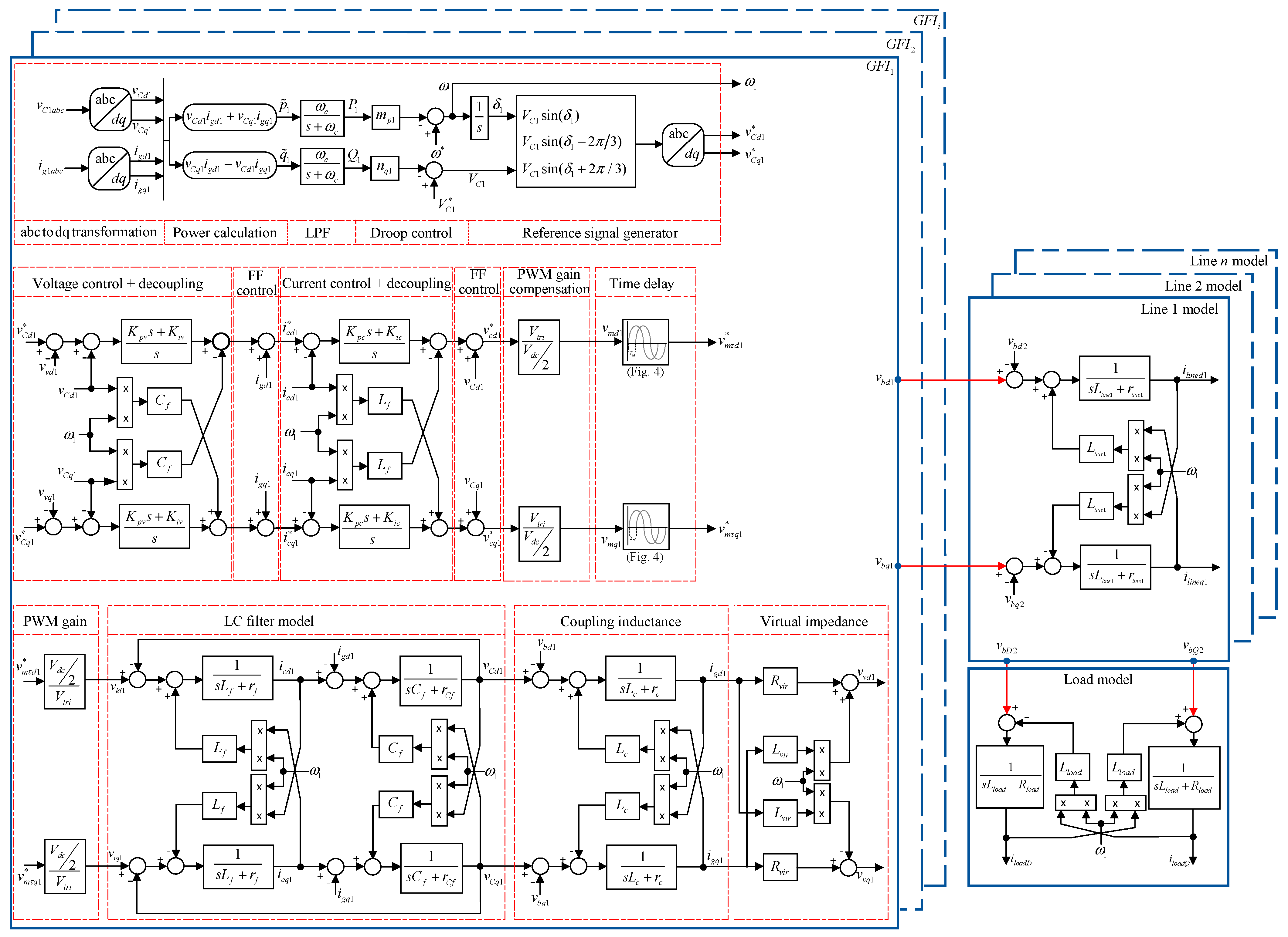
4.1. Small-Signal Model of Parallel-Connected GFIs

Each GFI in an island MG is modeled on its own reference frame, dq_i. However, to develop a complete small-signal model, its transformation into a common reference frame (DQ) is necessary. Therefore, all the reference frames (dq_i) in the MG are converted into a common reference frame (DQ), using the transformation matrix, T_i, as shown in Equation (21), where the lower-case dq_i indicates the reference frame for the i.th inverter, while the upper-case axes (DQ) indicate the common reference frame. The δ_i in Equation (21) [4] corresponds to the angle between the reference frame of the i.th GFI and the common reference frame. In this paper, the reference frame of the first GFI is chosen as the common reference frame, so ${\omega }_{\mathit{com}}={\omega }_{i=1}$ and ${\delta }_i=\int \left({\omega }_i-{\omega }_{\mathit{com}}\right)\mathit{dt}$.

$$f_{\mathit{DQi}}=\underset{T_i}{\underbrace{\left[\begin{array}{cc}\mathit{cos}\left({\delta }_i\right)& -\mathit{sin}\left({\delta }_i\right)\\ \mathit{sin}\left({\delta }_i\right)& \mathit{cos}\left({\delta }_i\right)\end{array}\right]}}{f}_{\mathit{dqi}}.$$

(21)

4.1.1. Power Controller Small-Signal Model

The active and reactive power derived from the inverter output current, i_gdq, and the capacitor voltage, v_Cdq, in regard to the dq-axis are given in Equation (22) [4], where $\stackrel{\mathrm{~}}{p}$ stands for instantaneous active power and $\stackrel{\mathrm{~}}{q}$ stands for instantaneous reactive power.

$$\begin{array}{c}\stackrel{\mathrm{~}}{p}=v_{\mathit{Cd}}{i}_{\mathit{gd}}+v_{\mathit{Cq}}{i}_{\mathit{gq}},\\ \stackrel{\mathrm{~}}{q}=v_{\mathit{Cq}}{i}_{\mathit{gd}} -v_{\mathit{Cd}}{i}_{\mathit{gq}}.\end{array}$$

(22)

In regard to droop control, active power $\stackrel{\mathrm{~}}{p}$ and $\stackrel{\mathrm{~}}{q}$ are filtered using a first-order low-pass filter (LPF), with the cut-off frequency, ω_c, as shown in Figure 7. Droop control equations for active and reactive power are provided in Equation (6). To develop small-signal models of the power controller, Equations (6), (21), and (22) are linearized around a certain operating point. The linearization results in Equation (23). In Equation (23), the capital letters, I_gd, I_gq, V_Cd, and V_Cq represent the grid current and capacitor voltage amplitudes at the operating point, and P and Q stand for filtered active and reactive power, respectively.

$$\begin{array}{c}\mathsf{\Delta }\dot{\delta }=-m_p\mathsf{\Delta }P-\mathsf{\Delta }{\omega }_{\mathit{com}}, \\ \mathsf{\Delta }\dot{P}={\omega }_c\left(-\mathsf{\Delta }P+I_{\mathit{gd}}\mathsf{\Delta }{v}_{\mathit{Cd}}+I_{\mathit{gq}}\mathsf{\Delta }{v}_{\mathit{Cq}}+V_{\mathit{Cd}}\mathsf{\Delta }{i}_{\mathit{gd}}+V_{\mathit{Cq}}\mathsf{\Delta }{i}_{\mathit{gq}}\right), \\ \mathsf{\Delta }\dot{Q}={\omega }_c\left(-\mathsf{\Delta }Q+I_{\mathit{gq}}\mathsf{\Delta }{v}_{\mathit{Cd}}-I_{\mathit{gd}}\mathsf{\Delta }{v}_{\mathit{Cq}}-V_{\mathit{Cq}}\mathsf{\Delta }{i}_{\mathit{gd}}+V_{\mathit{Cd}}\mathsf{\Delta }{i}_{\mathit{gq}}\right). \end{array}$$

(23)

When Equation (23) is organized in matrix form, a small-signal model of the power controller is obtained, as shown in Equation (24a) [4].

$$\begin{array}{c}\left[\begin{array}{c}\mathsf{\Delta }\dot{\delta }\\ \mathsf{\Delta }\dot{P}\\ \mathsf{\Delta }\dot{Q}\end{array}\right]=A_P\left[\begin{array}{c}\mathsf{\Delta }\delta \\ \mathsf{\Delta }P\\ \mathsf{\Delta }Q\end{array}\right]+B_P\left[\begin{array}{c}\mathsf{\Delta }{i}_{\mathit{cdq}}\\ \mathsf{\Delta }{v}_{\mathit{Cdq}}\\ \mathsf{\Delta }{i}_{\mathit{gdq}}\end{array}\right]+B_{P_{\omega \mathit{com}}}\left[\mathsf{\Delta }{\omega }_{\mathit{com}}\right],\\ \left[\begin{array}{c}\mathsf{\Delta }\omega \\ \mathsf{\Delta }{v}_{\mathit{Cd}}\\ \mathsf{\Delta }{v}_{\mathit{Cq}}\end{array}\right]=C_P\left[\begin{array}{c}\mathsf{\Delta }\delta \\ \mathsf{\Delta }P\\ \mathsf{\Delta }Q\end{array}\right].\end{array}$$

(24a)

The A_P, B_P, B_Pωcom, and C_P matrices in Equation (24a) are given below in Equation (24b) [4].

$$\begin{gathered} A_P=\left[\begin{array}{ccc}0& -m_p& 0\\ 0& -{\omega }_c& 0\\ 0& 0& -{\omega }_c\end{array}\right], B_P=\left[\begin{array}{cccccc}0& 0& 0& 0& 0& 0\\ 0& 0& {\omega }_c{I}_{\mathit{gd}}& {\omega }_c{I}_{\mathit{gq}}& {\omega }_c{V}_{\mathit{Cd}}& {\omega }_c{V}_{\mathit{Cq}}\\ 0& 0& -{\omega }_c{I}_{\mathit{gq}}& {\omega }_c{I}_{\mathit{gd}}& {\omega }_c{V}_{\mathit{Cq}}& -{\omega }_c{V}_{\mathit{Cd}}\end{array}\right], \\ {B}_{P_{\omega \mathit{com}}}=\left[\begin{array}{c}-1\\ 0\\ 0\end{array}\right], C_P=\left[\begin{array}{ccc}0& -m_p& 0\\ 0& 0& -n_q\\ 0& 0& 0\end{array}\right], C_P=\left[\begin{array}{c}{\left[C_{P_{\omega }}\right]}_{1\times 3}\\ {\left[C_{P_v}\right]}_{2\times 3}\end{array}\right]. \end{gathered}$$

(24b)

4.1.2. Voltage Controller Small-Signal Model

In regard to the voltage controller depicted in Figure 7, the capacitor voltage, $v_C$, is controlled using PI controllers in regard to the dq-axis, including cross-coupling terms and FF control. In Equation (25), ϕ_d and ϕ_q are presented as the state variables of the voltage controller, and $v_{\mathit{Cd}}^{\ast }$ and $v_{\mathit{Cq}}^{\ast }$ stand for d-axis and q-axis references for the voltage control loop.

$$\begin{array}{c}{\displaystyle \frac{d{\varphi }_d}{\mathit{dt}}}=v_{\mathit{Cd}}^{\ast }-v_{\mathit{Cd}},\\ {\displaystyle \frac{d{\varphi }_q}{\mathit{dt}}}=v_{\mathit{Cq}}^{\ast }-v_{\mathit{Cq}}.\end{array}$$

(25)

The reference currents, $i_{\mathit{Cd}}^{\ast }$ and $i_{\mathit{Cq}}^{\ast }$, in regard to the dq-axis at the output of the voltage controller are specified in Equation (26). In Equation (26), C_f is filter capacitance, and K_pv and K_iv are the proportional and integral coefficients of the voltage PI controller, respectively.

$$\begin{array}{c}{i}_{\mathit{cd}}^{\ast }=i_{\mathit{gd}}-\omega C_f{v}_{\mathit{Cq}}+K_{\mathit{pv}}\left(v_{\mathit{Cd}}^{\ast }-v_{\mathit{Cd}}\right)+K_{\mathit{iv}}{\displaystyle \frac{\left(v_{\mathit{Cd}}^{\ast }-v_{\mathit{Cd}}\right)}{s}},\\ i_{\mathit{cq}}^{\ast }=i_{\mathit{gq}}+\omega C_f{v}_{\mathit{Cd}}+K_{\mathit{pv}}\left(v_{\mathit{Cq}}^{\ast }-v_{\mathit{Cq}}\right)+K_{\mathit{iv}}{\displaystyle \frac{\left(v_{\mathit{Cq}}^{\ast }-v_{\mathit{Cq}}\right)}{s}}.\end{array}$$

(26)

The linearization of Equations (25) and (26) around a certain operating point results in Equation (27), where ω_o stands for the operating point value of the angular frequency.

$$\begin{array}{c}\mathsf{\Delta }{\dot{\varphi }}_d=\mathsf{\Delta }{v}_{\mathit{Cd}}^{\ast }-\mathsf{\Delta }{v}_{\mathit{Cd}}, \\ \mathsf{\Delta }{\dot{\varphi }}_q=\mathsf{\Delta }{v}_{\mathit{Cq}}^{\ast }-\mathsf{\Delta }{v}_{\mathit{Cq}},\\ \mathsf{\Delta }{i}_{\mathit{cd}}^{\ast }=K_{\mathit{iv}}\mathsf{\Delta }{\varphi }_d+K_{\mathit{pv}}\mathsf{\Delta }{v}_{\mathit{Cd}}^{\ast }-K_{\mathit{pv}}\mathsf{\Delta }{v}_{\mathit{Cd}} -{\omega }_o{C}_f\mathsf{\Delta }{v}_{\mathit{Cq}}-C_f{V}_{\mathit{Cq}}\mathsf{\Delta }\omega +\mathsf{\Delta }{i}_{\mathit{gd}}, \\ \mathsf{\Delta }{i}_{\mathit{cq}}^{\ast }=K_{\mathit{iv}}\mathsf{\Delta }{\varphi }_q+K_{\mathit{pv}}\mathsf{\Delta }{V}_{\mathit{Cq}}^{\ast }-K_{\mathit{pv}}\mathsf{\Delta }{v}_{\mathit{Cq}}+{\omega }_o{C}_f\mathsf{\Delta }{v}_{\mathit{Cd}}+C_f{V}_{\mathit{Cd}}\mathsf{\Delta }\omega +\mathsf{\Delta }{i}_{\mathit{gq}}. \end{array}$$

(27)

When Equation (27) is organized in matrix form, a small-signal model of the voltage controller is obtained, as shown in Equation (28a). It is important to note that, in the literature, the E_V matrix is missing. However, in this paper, in contrast to conventional modeling, ω is considered as a state variable, while linearization results in accurate small-signal modeling of the voltage controller, since the decoupling depends on the angular frequency, ω, which is overlooked in the literature for small-signal modeling.

$$\begin{array}{c}\left[\begin{array}{c}\mathsf{\Delta }{\dot{\varphi }}_d\\ \mathsf{\Delta }{\dot{\varphi }}_q\end{array}\right]={\left[0\right]}_{2 \times 2}\left[\begin{array}{c}\mathsf{\Delta }{\varphi }_d\\ \mathsf{\Delta }{\varphi }_q\end{array}\right]+B_{V1}\left[\begin{array}{c}\mathsf{\Delta }{v}_{\mathit{Cd}}^{\ast }\\ \mathsf{\Delta }{v}_{\mathit{Cq}}^{\ast }\end{array}\right]+B_{V2}\left[\begin{array}{c}\mathsf{\Delta }{i}_{\mathit{cdq}} \\ \mathsf{\Delta }{v}_{\mathit{Cdq}}\\ \mathsf{\Delta }{i}_{\mathit{gdq}}\end{array}\right], \\ \left[\begin{array}{c}\mathsf{\Delta }{i}_{\mathit{id}}^{\ast }\\ \mathsf{\Delta }{i}_{\mathit{iq}}^{\ast }\end{array}\right]=C_V\left[\begin{array}{c}\mathsf{\Delta }{\varphi }_d\\ \mathsf{\Delta }{\varphi }_q\end{array}\right]+D_{V1}\left[\begin{array}{c}\mathsf{\Delta }{v}_{\mathit{Cd}}^{\ast }\\ \mathsf{\Delta }{v}_{\mathit{Cq}}^{\ast }\end{array}\right]+D_{V2}\left[\begin{array}{c}\mathsf{\Delta }{i}_{\mathit{cdq}} \\ \mathsf{\Delta }{v}_{\mathit{Cdq}}\\ \mathsf{\Delta }{i}_{\mathit{gdq}}\end{array}\right]+E_V\left[\mathsf{\Delta }\omega \right].\end{array}$$

(28a)

The B_V1, B_V2, C_V, D_V1, D_V2, and E_V matrices in Equation (28a) are given below in Equation (28b):

$$\begin{gathered} B_{V1}=\left[\begin{array}{cc}1& 0\\ 0& 1\end{array}\right], B_{V2}=\left[\begin{array}{cccccc}0& 0& -1& 0& 0& 0\\ 0& 0& 0& -1& 0& 0\end{array}\right], C_V=\left[\begin{array}{cc}{K}_{\mathit{iv}}& 0\\ 0& K_{\mathit{iv}}\end{array}\right], D_{V1}=\left[\begin{array}{cc}{K}_{\mathit{pv}}& 0\\ 0& K_{\mathit{pv}}\end{array}\right], \\ {D}_{V2}=\left[\begin{array}{cccccc}0& 0& -K_{\mathit{pv}}& -{\omega }_o{C}_f& 1& 0\\ 0& 0& {\omega }_o{C}_f& -K_{\mathit{pv}}& 0& 1\end{array}\right], E_V=\left[\begin{array}{c}-C_f{V}_{\mathit{Cq}}\\ C_f{V}_{\mathit{Cd}}\end{array}\right]. \end{gathered}$$

(28b)

4.1.3. Current Controller Small-Signal Model

In regard to the current controller depicted in Figure 7, the converter-side filter inductance current, i_c, is controlled using a PI controller in regard to the dq-axis, including the cross-coupling terms and FF control. In Equation (29), γ_d and γ_q are presented as the state variables of the current controller, and $i_{\mathit{Cd}}^{\ast }$ and $i_{\mathit{Cq}}^{\ast }$ stand for the d-axis and q-axis references for the current control loop.

$$\begin{array}{c}{\displaystyle \frac{d{\gamma }_d}{\mathit{dt}}}=i_{\mathit{cd}}^{\ast }-i_{\mathit{cd}},\\ {\displaystyle \frac{d{\gamma }_q}{\mathit{dt}}}=i_{\mathit{cq}}^{\ast }-i_{\mathit{cq}}.\end{array}$$

(29)

The reference voltages, $v_{\mathit{id}}^{\ast }$ and $v_{\mathit{iq}}^{\ast }$, in regard to the dq-axis at the output of the current controller are specified in Equation (30). In Equation (30), L_f is filter inductance, and K_pc and K_ic are the proportional and integral coefficients of the current PI controller, respectively.

$$\begin{array}{c}{v}_{\mathit{id}}^{\ast }=-\omega L_f{i}_{\mathit{cq}}+K_{\mathit{pc}}\left(i_{\mathit{cd}}^{\ast }-i_{\mathit{cd}}\right)+K_{\mathit{ic}}{\displaystyle \frac{\left(i_{\mathit{cd}}^{\ast }-i_{\mathit{cd}}\right)}{s}}+v_{\mathit{Cd}},\\ v_{\mathit{iq}}^{\ast }=\omega L_f{i}_{\mathit{cd}}+K_{\mathit{pc}}\left(i_{\mathit{cq}}^{\ast }-i_{\mathit{cq}}\right)+K_{\mathit{ic}}{\displaystyle \frac{\left(i_{\mathit{cq}}^{\ast }-i_{\mathit{cq}}\right)}{s}}+v_{\mathit{Cq}}.\end{array}$$

(30)

The linearization of Equations (29) and (30) around a certain operating point results in Equation (31), where ω_o, I_cd, and I_cq stand for the angular frequency, d-axis and q-axis operating point values of the converter-side filter current, respectively.

When Equation (31) is organized in matrix form, a small-signal model of the current controller is obtained, as shown in Equation (32a). Similarly to the voltage controller small-signal model, in the literature, the E_C matrix is missing. However, in this paper, in contrast to conventional modeling, ω is considered as a state variable, while linearization results in accurate modeling of the current controller, since the decoupling depends on the angular frequency, ω, which is overlooked in the literature for small-signal modeling.

$$\begin{array}{c}\dot{\mathsf{\Delta }}{\gamma }_d=\mathsf{\Delta }{i}_{\mathit{cd}}^{\ast }-\mathsf{\Delta }{i}_{\mathit{cd}},\\ \mathsf{\Delta }{\dot{\gamma }}_q=\mathsf{\Delta }{i}_{\mathit{cq}}^{\ast }-\mathsf{\Delta }{i}_{\mathit{cq}},\\ \mathsf{\Delta }{v}_{\mathit{id}}^{\ast }=K_{\mathit{ic}}\mathsf{\Delta }{\gamma }_d+K_{\mathit{pc}}\mathsf{\Delta }{i}_{\mathit{cd}}^{\ast }-K_{\mathit{pc}}\mathsf{\Delta }{i}_{\mathit{cd}}-{\omega }_o{L}_f\mathsf{\Delta }{i}_{\mathit{cq}}-L_f{I}_{\mathit{cq}}\mathsf{\Delta }\omega +\mathsf{\Delta }{v}_{\mathit{cd}} \\ \mathsf{\Delta }{v}_{\mathit{iq}}^{\ast }=K_{\mathit{ic}}\mathsf{\Delta }{\gamma }_q+K_{\mathit{pc}}\mathsf{\Delta }{i}_{\mathit{cq}}^{\ast }-K_{\mathit{pc}}\mathsf{\Delta }{i}_{\mathit{cq}}+{\omega }_o{L}_f\mathsf{\Delta }{i}_{\mathit{cd}}+L_f{I}_{\mathit{cd}}\mathsf{\Delta }\omega +\mathsf{\Delta }{v}_{\mathit{cq}}.\end{array}$$

(31)

$$\begin{array}{c}\left[\begin{array}{c}\mathsf{\Delta }{\dot{\gamma }}_d\\ \mathsf{\Delta }{\dot{\gamma }}_q\end{array}\right]={\left[0\right]}_{2 \times 2}\left[\begin{array}{c}\mathsf{\Delta }{\gamma }_d\\ \mathsf{\Delta }{\gamma }_q\end{array}\right]+B_{C1}\left[\begin{array}{c}\mathsf{\Delta }{i}_{\mathit{cd}}^{\ast }\\ \mathsf{\Delta }{i}_{\mathit{cd}}^{\ast }\end{array}\right]+B_{C2}\left[\begin{array}{c}\mathsf{\Delta }{i}_{\mathit{cdq} }\\ \mathsf{\Delta }{v}_{\mathit{Cdq}}\\ \mathsf{\Delta }{i}_{\mathit{gdq}} \end{array}\right], \\ \left[\begin{array}{c}\mathsf{\Delta }{v}_{\mathit{id}}^{\ast }\\ \mathsf{\Delta }{v}_{\mathit{iq}}^{\ast }\end{array}\right]=C_C\left[\begin{array}{c}\mathsf{\Delta }{\gamma }_d\\ \mathsf{\Delta }{\gamma }_q\end{array}\right]+D_{C1}\left[\begin{array}{c}\mathsf{\Delta }{i}_{\mathit{cd}}^{\ast }\\ \mathsf{\Delta }{i}_{\mathit{cq}}^{\ast }\end{array}\right]+D_{C2}\left[\begin{array}{c}\mathsf{\Delta }{i}_{\mathit{cdq}} \\ \mathsf{\Delta }{v}_{\mathit{Cdq}}\\ \mathsf{\Delta }{i}_{\mathit{gdq} }\end{array}\right]+E_C\left[\mathsf{\Delta }\omega \right].\end{array}$$

(32a)

The B_C1, B_C2, C_C, D_C1, D_C2, and E_C matrices in Equation (32a) are given below in Equation (32b):

$$\begin{gathered} B_{C1}=\left[\begin{array}{cc}1& 0\\ 0& 1\end{array}\right], B_{C2}=\left[\begin{array}{cccccc}-1& 0& 0& 0& 0& 0\\ 0& -1& 0& 0& 0& 0\end{array}\right], C_C=\left[\begin{array}{cc}{K}_{\mathit{ic}}& 0\\ 0& K_{\mathit{ic}}\end{array}\right], D_{C1}=\left[\begin{array}{cc}{K}_{\mathit{pc}}& 0\\ 0& K_{\mathit{pc}}\end{array}\right], \\ {D}_{C2}=\left[\begin{array}{cccccc}-K_{\mathit{pc}}& -{\omega }_o{L}_f& 1& 0& 0& 0\\ {\omega }_o{L}_f& -K_{\mathit{pc}}& 0& 1& 0& 0\end{array}\right], E_C=\left[\begin{array}{c}-L_f{I}_{cq}\\ L_f{I}_{cd}\end{array}\right]. \end{gathered}$$

(32b)

4.1.4. Virtual Impedance Small-Signal Model

A block diagram of the virtual impedance model is depicted in Figure 7. The voltage drop due to virtual impedance in regard to the dq-axis is given by Equation (33) [54]. In Equation (33), R_v and L_v are the virtual resistance and virtual inductance, respectively.

$$\begin{array}{c}{v}_{\mathit{vd}}=R_v{i}_{\mathit{gd}}-\omega L_v{i}_{\mathit{gq}}, \\ v_{\mathit{vq}}=R_v{i}_{\mathit{gq}}+\omega L_v{i}_{\mathit{gd}}.\end{array}$$

(33)

If the linearization process is applied to Equation (33), the following Equation (34) is obtained as given below.

$$\begin{array}{c}{v}_{\mathit{vd}}=R_v\mathsf{\Delta }{i}_{\mathit{gd}}-{\omega }_o{L}_v\mathsf{\Delta }{i}_{\mathit{gq}}-L_v{I}_{\mathit{gq}}\mathsf{\Delta }\omega ,\\ v_{\mathit{vq}}=R_v\mathsf{\Delta }{i}_{\mathit{gq}}+{\omega }_o{L}_v\mathsf{\Delta }{i}_{\mathit{gd}}+L_v{I}_{\mathit{gd}}\mathsf{\Delta }\omega .\end{array}$$

(34)

When Equation (34) is arranged in matrix form, the virtual impedance small-signal model is as detailed in Equation (35a).

$$\left[\begin{array}{c}{v}_{\mathit{vd}}\\ v_{\mathit{vq}}\end{array}\right]=A_z\left[\begin{array}{c}\mathsf{\Delta }{i}_{\mathit{cdq}}\\ \mathsf{\Delta }{v}_{\mathit{Cdq}}\\ \mathsf{\Delta }{i}_{\mathit{gdq}}\end{array}\right]+B_z\left[\begin{array}{c}-L_v{I}_{\mathit{gq}}\\ L_v{I}_{\mathit{gd}}\end{array}\right]\left[\mathsf{\Delta }\omega \right].$$

(35a)

The A_z and B_z matrices in Equation (35a) are given below in Equation (35b):

$$A_z=\left[\begin{array}{cccccc}0& 0& 0& 0& R_v& {\omega }_o{L}_v\\ 0& 0& 0& 0& -{\omega }_o{L}_v& R_v\end{array}\right],B_z=\left[\begin{array}{c}-L_v{I}_{\mathit{oq}}\\ L_v{I}_{\mathit{od}}\end{array}\right]$$

(35b)

4.1.5. LC Filter and Coupling Inductance Small-Signal Model

In Equation (36), the differential equation of the LC filter and coupling inductance model depicted in Figure 7 are given in regard to the dq-axis. Here, it is assumed that the LCL filter input voltage, $v_{\mathit{idq}}$, is equal to the output of the time delay, $v_{\tau dq}^{\ast }$. When the linearization process is applied to Equation (36), it becomes Equation (37) as given below.

$$\begin{array}{c}{\displaystyle \frac{d{i}_{\mathit{id}}}{\mathit{dt}}}={\displaystyle \frac{-r_f}{L_f}}{i}_{\mathit{cd}}+\omega i_{\mathit{cq}}+{\displaystyle \frac{1}{L_f}}{v}_{\mathit{id}}-{\displaystyle \frac{1}{L_f}}{v}_{\mathit{Cd}},\\ {\displaystyle \frac{d{i}_{\mathit{iq}}}{\mathit{dt}}}={\displaystyle \frac{-r_f}{L_f}}{i}_{\mathit{cq}}-\omega i_{\mathit{cd}}+{\displaystyle \frac{1}{L_f}}{v}_{\mathit{iq}}-{\displaystyle \frac{1}{L_f}}{v}_{\mathit{Cq},}\\ {\displaystyle \frac{d{v}_{\mathit{Cd}}}{\mathit{dt}}}=\omega v_{\mathit{Cq}}+\left({\displaystyle \frac{1}{C_f}}-{\displaystyle \frac{r_{C_f}{r}_f}{L_f}}\right)i_{\mathit{cd}}+\left({\displaystyle \frac{-r_{C_f}}{L_f}}-{\displaystyle \frac{r_{C_f}}{L_c}}\right)v_{\mathit{Cd}}+\left({\displaystyle \frac{-1}{C_f}}+{\displaystyle \frac{r_{C_f}{r}_c}{L_c}}\right)i_{\mathit{gd}}+{\displaystyle \frac{r_{C_f}}{L_c}}{v}_{\mathit{bd}}+{\displaystyle \frac{r_{C_f}}{L_f}}{v}_{\mathit{id}},\\ {\displaystyle \frac{d{v}_{\mathit{Cq}}}{\mathit{dt}}}=-\omega v_{\mathit{Cd}}+\left({\displaystyle \frac{1}{C_f}}-{\displaystyle \frac{r_{C_f}{r}_f}{L_f}}\right)i_{\mathit{cq}}+\left({\displaystyle \frac{-r_{C_f}}{L_f}}-{\displaystyle \frac{r_{C_f}}{L_c}}\right)v_{\mathit{Cd}}+\left({\displaystyle \frac{-1}{C_f}}+{\displaystyle \frac{r_{C_f}{r}_c}{L_c}}\right)i_{\mathit{cq}}+{\displaystyle \frac{r_{C_f}}{L_c}}{v}_{\mathit{bq}}+{\displaystyle \frac{r_{C_f}}{L_f}}{v}_{\mathit{iq}}, \\ {\displaystyle \frac{d{i}_{\mathit{gd}}}{\mathit{dt}}}={\displaystyle \frac{-r_c}{L_c}}{i}_{\mathit{gd}}+\omega i_{\mathit{gq}}+{\displaystyle \frac{1}{L_c}}{v}_{\mathit{Cd}}-{\displaystyle \frac{1}{L_c}}{v}_{\mathit{bd}},\\ {\displaystyle \frac{d{i}_{\mathit{gq}}}{\mathit{dt}}}={\displaystyle \frac{-r_c}{L_c}}{i}_{\mathit{gq}}-\omega i_{\mathit{gd}}+{\displaystyle \frac{1}{L_c}}{v}_{\mathit{Cq}}-{\displaystyle \frac{1}{L_c}}{v}_{\mathit{bq}}.\end{array}$$

(36)

In Equation (36), i_cd, i_cq, L_f, C_f, r_f, r_Cf, i_gd, and i_gq are the d-axis converter-side current, the q-axis converter-side current, filter inductance, filter capacitance, the parasitic resistance of L_f, the parasitic resistance of C_f, the d-axis grid-side current, and the q-axis grid-side current, respectively.

$$\begin{array}{c}\mathsf{\Delta }{\dot{i}}_{\mathit{cd}}={\displaystyle \frac{-r_f}{L_f}}\mathsf{\Delta }{i}_{\mathit{cd}}+{\omega }_o\mathsf{\Delta }{i}_{\mathit{cq}}+{\displaystyle \frac{1}{L_f}}\mathsf{\Delta }{v}_{\mathit{id}}-{\displaystyle \frac{1}{L_f}}\mathsf{\Delta }{v}_{\mathit{Cd}}+I_{\mathit{cq}}\mathsf{\Delta }\omega ,\\ \mathsf{\Delta }{\dot{i}}_{\mathit{cq}}={\displaystyle \frac{-r_f}{L_f}}\mathsf{\Delta }{i}_{\mathit{cq}}-{\omega }_o\mathsf{\Delta }{i}_{\mathit{cd}}+{\displaystyle \frac{1}{L_f}}\mathsf{\Delta }{v}_{\mathit{iq}}-{\displaystyle \frac{1}{L_f}}\mathsf{\Delta }{v}_{\mathit{Cq}}-I_{\mathit{cd}}\mathsf{\Delta }\omega ,\\ \mathsf{\Delta }{\dot{v}}_{\mathit{Cd}}={\omega }_o\mathsf{\Delta }{v}_{\mathit{Cq}}+\left({\displaystyle \frac{1}{C_f}}-{\displaystyle \frac{r_{C_f}{r}_f}{L_f}}\right)\mathsf{\Delta }{i}_{\mathit{cd}}+\left({\displaystyle \frac{-r_{C_f}}{L_f}}-{\displaystyle \frac{r_{C_f}}{L_c}}\right)\mathsf{\Delta }{v}_{\mathit{Cd}}+\left({\displaystyle \frac{-1}{C_f}}+{\displaystyle \frac{r_{C_f}{r}_c}{L_c}}\right)\mathsf{\Delta }{i}_{\mathit{gd}}+{\displaystyle \frac{r_{C_f}}{L_c}}\mathsf{\Delta }{v}_{\mathit{bd}}+{\displaystyle \frac{r_{C_f}}{L_f}}\mathsf{\Delta }{v}_{\mathit{id}}+V_{\mathit{Cq}}\mathsf{\Delta }\omega \\ \mathsf{\Delta }{\dot{v}}_{\mathit{Cq}}=-{\omega }_o\mathsf{\Delta }{v}_{\mathit{Cd}}+\left({\displaystyle \frac{1}{C_f}}-{\displaystyle \frac{r_{C_f}{r}_f}{L_f}}\right)\mathsf{\Delta }{i}_{\mathit{cq}}+\left({\displaystyle \frac{-r_{C_f}}{L_f}}-{\displaystyle \frac{r_{C_f}}{L_c}}\right)\mathsf{\Delta }{v}_{\mathit{Cq}}+\left({\displaystyle \frac{-1}{C_f}}+{\displaystyle \frac{r_{C_f}{r}_c}{L_c}}\right)\mathsf{\Delta }{i}_{\mathit{gq}}+{\displaystyle \frac{r_{C_f}}{L_c}}\mathsf{\Delta }{v}_{\mathit{bq}}+{\displaystyle \frac{r_{C_f}}{L_f}}\mathsf{\Delta }{v}_{\mathit{iq}}-V_{\mathit{Cd}}\mathsf{\Delta }\omega ,\\ \mathsf{\Delta }{\dot{i}}_{\mathit{gd}}={\displaystyle \frac{-r_c}{L_c}}\mathsf{\Delta }{i}_{\mathit{gd}}+{\omega }_o\mathsf{\Delta }{i}_{\mathit{gq}}+{\displaystyle \frac{1}{L_c}}\mathsf{\Delta }{v}_{\mathit{Cd}}-{\displaystyle \frac{1}{L_c}}\mathsf{\Delta }{v}_{\mathit{bd}}+I_{\mathit{gq}}\mathsf{\Delta }\omega ,\\ \mathsf{\Delta }{\dot{i}}_{\mathit{gq}}={\displaystyle \frac{-r_c}{L_c}}\mathsf{\Delta }{i}_{\mathit{gq}}-{\omega }_o\mathsf{\Delta }{i}_{\mathit{gd}}+{\displaystyle \frac{1}{L_c}}\mathsf{\Delta }{v}_{\mathit{Cq}}-{\displaystyle \frac{1}{L_c}}\mathsf{\Delta }{v}_{\mathit{bq}}-I_{\mathit{gd}}\mathsf{\Delta }\omega .\end{array}$$

(37)

By arranging Equation (37) in matrix form, the small-signal model of the LC filter and coupling inductance are obtained, as in Equation (38a). The A_LCL, B_LCL1, B_LCL2, and B_LCL3 matrices in Equation (38a) are given below in Equation (38b). V_Cd and V_Cq are the d-axis and q-axis operating point values for the filter capacitance voltage, respectively.

$$\left[\begin{array}{c}\mathsf{\Delta }{\dot{i}}_{\mathit{cdq} }\\ \mathsf{\Delta }{\dot{v}}_{\mathit{Cdq}}\\ \mathsf{\Delta }{\dot{i}}_{\mathit{gdq}}\end{array}\right]=\begin{array}{c}{A}_{\mathit{LCL}}\left[\begin{array}{c}\mathsf{\Delta }{i}_{\mathit{cdq}}\\ \mathsf{\Delta }{v}_{\mathit{Cdq}}\\ \mathsf{\Delta }{i}_{\mathit{gdq}}\end{array}\right]+B_{\mathit{LCL}1}\left[\mathsf{\Delta }{v}_{\mathrm{idq}}\right] +B_{\mathit{LCL}2}\left[\mathsf{\Delta }{v}_{\mathit{bdq}}\right]+B_{\mathit{LCL}3}\left[\mathsf{\Delta }\omega \right].\end{array}$$

(38a)

$$\begin{gathered} A_{\mathit{LCL}}=\left[\begin{array}{cccccc}{\displaystyle \frac{-r_f}{L_f}}& {\omega }_o& {\displaystyle \frac{-1}{L_f}}& 0& 0& 0\\ -{\omega }_o& {\displaystyle \frac{-r_f}{L_f}}& 0& {\displaystyle \frac{-1}{L_f}}& 0& 0\\ \left({\displaystyle \frac{1}{C_f}}-{\displaystyle \frac{r_{C_f}{r}_f}{L_f}}\right)& 0& \left({\displaystyle \frac{-r_{C_f}}{L_f}}-{\displaystyle \frac{r_{C_f}}{L_c}}\right)& {\omega }_o& \left({\displaystyle \frac{-1}{C_f}}+{\displaystyle \frac{r_{C_f}{r}_c}{L_c}}\right)& 0\\ 0& \left({\displaystyle \frac{1}{C_f}}-{\displaystyle \frac{r_{C_f}{r}_f}{L_f}}\right)& -{\omega }_o& \left({\displaystyle \frac{-r_{C_f}}{L_f}}-{\displaystyle \frac{r_{C_f}}{L_c}}\right)& 0& \left({\displaystyle \frac{-1}{C_f}}+{\displaystyle \frac{r_{C_f}{r}_c}{L_c}}\right)\\ 0& 0& {\displaystyle \frac{1}{L_c}}& 0& {\displaystyle \frac{-r_c}{L_c}}& {\omega }_o\\ 0& 0& 0& {\displaystyle \frac{1}{L_c}}& -{\omega }_o& {\displaystyle \frac{-r_c}{L_c}}\end{array}\right], \\ {B}_{\mathit{LCL}1}={\left[\begin{array}{cccccc}{\displaystyle \frac{1}{L_f}}& 0& {\displaystyle \frac{r_{C_f}}{L_f}}& 0& 0& 0\\ 0& {\displaystyle \frac{1}{L_f}}& 0& {\displaystyle \frac{r_{C_f}}{L_f}}& 0& 0\end{array}\right], }^T{B}_{\mathit{LCL}2}={\left[\begin{array}{cccccc}0& 0& {\displaystyle \frac{r_{C_f}}{L_c}}& 0& {\displaystyle \frac{-1}{L_c}}& 0\\ 0& 0& 0& {\displaystyle \frac{r_{C_f}}{L_c}}& 0& {\displaystyle \frac{-1}{L_c}}\end{array}\right]}^T \\ {B}_{\mathit{LCL}3}={\left[\begin{array}{cccccc}{\mathrm{I}}_{\mathit{cq}}& -{\mathrm{I}}_{\mathit{cd}}& {\mathrm{V}}_{\mathit{cq}}& -{\mathrm{V}}_{\mathit{cd}}& {\mathrm{I}}_{\mathit{gq}}& -{\mathrm{I}}_{\mathit{gd}}\end{array}\right]}^T. \end{gathered}$$

(38b)

4.1.6. Small-Signal Model of a GFI

The grid-side current, i_gDQ, can be obtained in regard to the common reference frame using the transformation matrix $T_i$ as given in Equation (39) [4].

$$\begin{array}{c}{i}_{\mathit{gD}}=\mathit{cos}\left(\delta \right)i_{\mathit{gd}}-\mathit{sin}\left(\delta \right)i_{\mathit{gq}},\\ i_{\mathit{gQ}}=\mathit{sin}\left(\delta \right)i_{\mathit{gd}}+\mathit{cos}\left(\delta \right)i_{\mathit{gq}}.\end{array}$$

(39)

If the linearization is applied to Equation (39), the following Equation (40) is obtained. In Equation (40), I_gd and I_gq are the operating point values of the grid-side currents.

$$\begin{array}{c}\mathsf{\Delta }{i}_{\mathit{gD}}=\mathit{cos}\left({\delta }_o\right)\mathsf{\Delta }{i}_{\mathit{gd}}-\mathit{sin}\left({\delta }_o\right)\mathsf{\Delta }{i}_{\mathit{gq}}+\left(-I_{\mathit{gd}}\mathit{sin}\left({\delta }_o\right)-I_{\mathit{gq}}\mathit{cos}\left({\delta }_o\right)\right)\mathsf{\Delta }\delta , \\ \mathsf{\Delta }{i}_{\mathit{gQ}}=\mathit{sin}\left({\delta }_o\right)\mathsf{\Delta }{i}_{\mathit{gq}}+\mathit{cos}\left({\delta }_o\right)\mathsf{\Delta }{i}_{\mathit{gq}}+\left(I_{\mathit{gd}}\mathit{cos}\left({\delta }_o\right)-I_{\mathit{gq}}\mathit{sin}\left({\delta }_o\right)\right)\mathsf{\Delta }\delta .\end{array}$$

(40)

If Equation (40) is arranged in matrix form, Equation (41a) is obtained as follows.

$$\left[\mathsf{\Delta }{i}_{\mathit{gDQ}}\right]=T_s\left[\mathsf{\Delta }{i}_{\mathit{gdq}}\right]+T_c\left[\mathsf{\Delta }\delta \right].$$

(41a)

The T_s and T_c matrices in Equation (41a) are given below in Equation (41b):

$$T_s=\left[\begin{array}{cc}\mathit{cos}\left({\delta }_o\right)& -\mathit{sin}\left({\delta }_o\right)\\ \mathit{sin}\left({\delta }_o\right)& \mathit{cos}\left({\delta }_o\right)\end{array}\right], T_c=\left[\begin{array}{c}-I_{\mathit{gd}}\mathit{sin}\left({\delta }_o\right)-I_{\mathit{gq}}\mathit{cos}\left({\delta }_o\right)\\ I_{\mathit{gd}}\mathit{cos}\left({\delta }_o\right)-I_{\mathit{gq}}\mathit{sin}\left({\delta }_o\right)\end{array}\right]$$

(41b)

Similarly, the bus voltage, v_bDQ, which is measured in regard to the common reference frame (DQ) should be converted into the GFIi’s own reference frame, dq_i, to develop the entire GFI small-signal model. Therefore, the inverse of the T_i matrix is used from the common reference frame in regard to the GFI’s reference frame, as shown in Equation (42).

$$\left[\begin{array}{c}{v}_{\mathit{bd}}\\ v_{\mathit{bq}}\end{array}\right]=\left[\begin{array}{cc}\mathit{cos}\left(\delta \right)& \mathit{sin}\left(\delta \right)\\ -\mathit{sin}\left(\delta \right)& \mathit{cos}\left(\delta \right)\end{array}\right]\left[\begin{array}{c}{v}_{\mathit{bD}}\\ v_{\mathit{bQ}}\end{array}\right].$$

(42)

From Equation (42), the equations for the bus voltage, $v_{bdq}$, in regard to the reference frame dq_i of GFI_i are given in Equation (43).

$$\begin{array}{c}{v}_{\mathit{bd}}=\mathit{cos}\left(\delta \right)v_{\mathit{bD}}+\mathit{sin}\left(\delta \right)v_{\mathit{bD}},\\ v_{\mathit{bq}}=-\mathit{sin}\left(\delta \right)v_{\mathit{bD}}+\mathit{cos}\left(\delta \right)v_{\mathit{bQ}}.\end{array}$$

(43)

If the linearization is applied to Equation (43), the following Equation (44) is obtained.

$$\begin{array}{c}\mathsf{\Delta }{v}_{\mathit{bd}}=\mathit{cos}\left({\delta }_o\right)\mathsf{\Delta }{v}_{\mathit{bD}}+\mathit{sin}\left({\delta }_o\right)\mathsf{\Delta }{v}_{\mathit{bQ}}+\left(-V_{\mathit{bD}}\mathit{sin}\left({\delta }_o\right)+V_{\mathit{bQ}}\mathit{cos}\left({\delta }_o\right)\right)\mathsf{\Delta }\delta ,\\ \mathsf{\Delta }{v}_{\mathit{bq}}=-\mathit{sin}\left({\delta }_o\right)\mathsf{\Delta }{v}_{\mathit{bD}}+\mathit{cos}\left({\delta }_o\right)\mathsf{\Delta }{v}_{\mathit{bQ}}+\left(-V_{\mathit{bD}}\mathit{cos}\left({\delta }_o\right)-V_{\mathit{bQ}}\mathit{sin}\left({\delta }_o\right)\right)\mathsf{\Delta }\delta .\end{array}$$

(44)

If Equation (44) is arranged in matrix form, the following Equation (45a) [4] is obtained:

$$\left[\mathsf{\Delta }{v}_{\mathit{bdq}}\right]=T_s^{-1}\left[\mathsf{\Delta }{v}_{\mathit{bDQ}}\right]+T_V^{-1}\left[\mathsf{\Delta }\delta \right].$$

(45a)

The $T_V^{-1}$ matrix in Equation (45a) is given below in Equation (45b).

$$T_V^{-1}=\left[\begin{array}{c}-V_{\mathit{bD}}\mathit{sin}\left({\delta }_o\right)+V_{\mathit{bQ}}\mathit{cos}\left({\delta }_o\right)\\ -V_{\mathit{bD}}\mathit{cos}\left({\delta }_o\right)-V_{\mathit{bQ}}\mathit{sin}\left({\delta }_o\right)\end{array}\right].$$

(45b)

The complete small-signal model of a GFI is obtained by combining the small-signal models of the power controller (Equation (24)), voltage controller (Equation (28)), current controller (Equation (32)), the proposed time delay model (Equation (20)), virtual impedance model (Equation (35)), and LC filter and coupling inductance model (Equation (38)). In this case, the GFI has a total of 21 state variables, Δx_GFIi = [Δδ_i ΔP_i ΔQ_i Δφ_dqi Δγ_dqi Δτ_dqki Δi_cdqi Δv_Cdqi Δi_gdqi]^T, three inputs, such as Δv_bdq and Δω_com, and two outputs, such as Δi_gdq. Exceptionally, only the GFI whose reference frame is selected as a common reference frame has three output variables, such as Δi_gdq and Δω_com. Consequently, the entire small-signal model of the GFI considering all the state variables is given in Equation (46).

$$\begin{array}{c}\mathsf{\Delta }{\dot{x}}_{\mathit{GFIi}}=A_{\mathit{GFIi}}\left[\mathsf{\Delta }{x}_{\mathit{GFIi}}\right]+B_{\mathit{GFIi}}\left[\mathsf{\Delta }{v}_{\mathit{bDQi}}\right]+B_{\omega \mathit{comi}}\left[\mathsf{\Delta }{\omega }_{\mathit{com}}\right],\\ \left[\begin{array}{c}\mathsf{\Delta }{\omega }_i \\ \mathsf{\Delta }{i}_{\mathit{gDQi}}\end{array}\right]=\left[\begin{array}{c}{C}_{\mathit{GFI}\omega i}\\ C_{\mathit{GFIci}}\end{array}\right]\left[\mathsf{\Delta }{x}_{\mathit{GFIi}}\right]. \end{array}$$

(46a)

$A_{\mathit{GFIi}}$, $B_{\mathit{GFIi}}$, $B_{\omega \mathit{comi}}$, $C_{\mathit{GFI}\omega i}$, and $C_{\mathit{GFIci}}$ in Equation (46a) are given below in Equation (46b):

$$\begin{gathered} A_{\mathit{GFIi}}=\left[\begin{array}{ccccc}{A}_{\mathit{Pi}}& 0_{3\times 2}& 0_{3\times 2}& 0_{3\times 8}& B_{\mathit{Pi}}\\ B_{V1i}{C}_{\mathit{Pvi}}-B_{V1i}{B}_{\mathit{Zi}}{C}_{P\omega i}& 0_{2\times 2}& 0_{2\times 2}& 0_{2\times 8}& B_{V2i}-B_{V1i}{A}_{\mathit{Zi}}\\ \left(\begin{array}{c}{B}_{C1i}{D}_{V1i}{C}_{\mathit{Pvi}}+B_{C1i}{E}_{\mathit{Vi}}{C}_{P\omega i}\\ -B_{C1i}{D}_{V1i}{B}_{\mathit{Zi}}{C}_{P\omega i}\end{array}\right)& B_{C1i}{C}_{\mathit{Vi}}& 0_{2\times 2}& 0_{2\times 8}& \left(\begin{array}{c}{B}_{C1i}{D}_{V2i}\\ +B_{C2i}-B_{C1i}{D}_{V1i}{A}_{\mathit{Zi}}\end{array}\right)\\ \left(\begin{array}{c}{B}_{\tau i}{D}_{C1i}{D}_{V1i}{C}_{\mathit{Pvi}}\\ -B_{\tau i}{D}_{C1i}{D}_{V1i}{B}_{\mathit{Zi}}{C}_{P\omega i}\\ +B_{\tau i}{D}_{C1i}{E}_{\mathit{Vi}}{C}_{P\omega i}+B_{\tau i}{E}_{\mathit{Ci}}{C}_{P\omega i}\end{array}\right)& B_{\tau i}{D}_{C1i}{C}_{\mathit{Vi}}& B_{\tau i}{C}_{\mathit{Ci}}& A_{\tau i}& \left(\begin{array}{c}{B}_{\tau i}{D}_{C1i}{D}_{V2i}\\ \&+B_{\tau i}{D}_{C2i}\\ -B_{\tau i}{D}_{C1i}{D}_{V1i}{A}_{\mathit{Zi}}\end{array}\right)\\ \left(\begin{array}{c}{B}_{\mathit{LCL}1i}{E}_{\tau i}{D}_{\tau i}{D}_{C1i}{D}_{V1i}{C}_{\mathit{Pvi}}\\ +B_{\mathit{LCL}1i}{E}_{\tau i}{D}_{\tau i}{D}_{C1i}{E}_{\mathit{Vi}}{C}_{P\omega i}\\ +B_{\mathit{LCL}1i}{E}_{\tau i}{D}_{\tau i}{E}_{\mathit{Ci}}{C}_{P\omega i}\\ +B_{\mathit{LCL}1i}{F}_{\tau i}{C}_{P\omega i}\\ +B_{\mathit{LCL}1i}{E}_{\tau i}{D}_{\tau i}{D}_{C1i}{D}_{V1i}{B}_{\mathit{Zi}}{C}_{P\omega i}\\ +B_{\mathit{LCL}2i}\left[T_{\mathit{Vi}}^{-1}{0}_{2\times 2}\right]+B_{\mathit{LCL}3i}{C}_{P\omega i}\end{array}\right)& B_{\mathit{LCL}1i}{E}_{\tau i}{D}_{\tau i}{D}_{C1i}{C}_{\mathit{Vi}}& B_{\mathit{LCL}1i}{E}_{\tau i}{D}_{\tau i}{C}_{\mathit{Ci}}& B_{\mathit{LCL}1}{E}_{\tau i}{C}_{\tau i}& \left(\begin{array}{c}{A}_{\mathrm{LCLi}}\\ +B_{\mathit{LCL}1i}{E}_{\tau i}{D}_{\tau i}{D}_{C1i}{D}_{V2i}\\ -B_{\mathit{LCL}1i}{E}_{\tau i}{D}_{\tau i}{D}_{C1i}{D}_{V1i}{A}_z\\ +B_{\mathit{LCL}1}{E}_{\mathit{td}}{D}_{\mathit{td}}{D}_{c2}\end{array}\right)\end{array}\right], \\ {B}_{\mathit{GFIi}}={\left[\begin{array}{c}{\left[0\right]}_{7\times 2}\\ B_{\mathit{LCL}2i}{T}_{\mathit{Si}}^{-1}\end{array}\right]}_{13\times 2}, B_{\omega \mathit{comi}}={\left[\begin{array}{c}{B}_{P\omega \mathit{com}}\\ {\left[0\right]}_{10\times 1}\end{array}\right]}_{13\times 1}, C_{\mathit{GFI}\omega i}=\left(\begin{array}{c}{\left[\begin{array}{cccc}{C}_{P\omega }& 0& ...& 0\end{array}\right]}_{1 \times 13},i=1\\ {\left[0\right]}_{1\times 13} ,i\ne 1\end{array}\right., \\ {C}_{\mathit{GFIci}}={\left[\begin{array}{ccc}{T}_{\mathit{Ci}}& {\left[0\right]}_{2\times 10}& T_{\mathit{Si}}\end{array}\right]}_{2 \times 13}. \end{gathered}$$

(46b)

In an island MG, there may be multiple GFIs. Therefore, it is necessary to develop a complete small-signal model for the GFIs in regard to a common reference frame. The state-space representation of the small-signal model for all the GFIs in the MG is given by Equation (47a).

$$\begin{array}{c}\mathsf{\Delta }{\dot{x}}_{\mathit{GFI}}=A_{\mathit{GFI}}\left[\mathsf{\Delta }{x}_{\mathit{GFI}}\right]+B_{\mathit{GFI}}\left[\mathsf{\Delta }{v}_{\mathit{bDQ}}\right],\\ \left[\mathsf{\Delta }{i}_{\mathit{gDQ}}\right]=C_{\mathit{GFIc}}\left[\mathsf{\Delta }{x}_{\mathit{GFI}}\right].\end{array}$$

(47a)

The ∆x_GFI, A_GFI, B_GFI, and C_GFIc matrices in Equation (47a) are given below in Equation (47b):

$$\begin{gathered} \left[\mathsf{\Delta }{x}_{\mathit{GFI}}\right]={\left[\begin{array}{cc}\mathsf{\Delta }{x}_{\mathit{GFI}1}& \mathsf{\Delta }{x}_{\mathit{GFI}2}\end{array}\right]}_{42 \times 42}^T, \left[\mathsf{\Delta }{v}_{\mathit{bDQ}}\right]={\left[\begin{array}{ccc}\mathsf{\Delta }{v}_{\mathit{bDQ}1}& \mathsf{\Delta }{v}_{\mathit{bDQ}2}& \mathsf{\Delta }{v}_{\mathit{bDQ}2}\end{array}\right]}_{6 \times 1}^T, \\ {A}_{\mathit{GFI}}={\left[\begin{array}{cc}{A}_{\mathit{GFI}1}+B_{1\omega \mathit{com}}{C}_{\mathit{GFI}\omega 1}& 0_{21 \times 21}\\ B_{\omega \mathit{com}1}{C}_{\mathit{GFI}\omega 1}& A_{\mathit{GFI}2}\end{array}\right]}_{42 \times 42}, B_{\mathit{GFI}}={\left[\begin{array}{ccc}{B}_{\mathit{GFI}1}& 0_{21 \times 2}& 0_{21 \times 2}\\ 0_{21 \times 2}& 0_{21 \times 2}& B_{\mathit{GFI}2}\end{array}\right]}_{42 \times 6}, \\ {C}_{\mathit{GFIc}}={\left[\begin{array}{cc}{C}_{\mathit{GFIc}1}& 0_{2 \times 21}\\ 0_{2 \times 21}& C_{\mathit{GFIc}2}\end{array}\right]}_{4 \times 42}. \end{gathered}$$

(47b)

4.2. Transmission Line Small-Signal Model

The generalized differential equations of the transmission line connected between bus j and bus k in regard to the common reference frame (DQ) are given in Equation (48) [4], where n is the number of lines, m is the number of buses, i is the number of inverters, and p is the number of loads, and r_line and L_line are the resistance and inductance of the transmission line, respectively.

$$\begin{array}{c}{\displaystyle \frac{d{i}_{\mathit{lineDn}}}{\mathit{dt}}}={\displaystyle \frac{-r_{\mathit{linei}}}{L_{\mathit{linei}}}}{i}_{\mathit{lineDn}}+\omega i_{\mathit{lineQn}}+{\displaystyle \frac{1}{L_{\mathit{linei}}}}{v}_{\mathit{bDj}}-{\displaystyle \frac{1}{L_{\mathit{linei}}}}{v}_{\mathit{bDk}},\\ {\displaystyle \frac{d{i}_{\mathit{lineQn}}}{\mathit{dt}}}={\displaystyle \frac{-r_{\mathit{linei}}}{L_{\mathit{linei}}}}{i}_{\mathit{lineQn}}-\omega i_{\mathit{lineDn}}+{\displaystyle \frac{1}{L_{\mathit{linei}}}}{v}_{\mathit{bQj}}-{\displaystyle \frac{1}{L_{\mathit{linei}}}}{v}_{\mathit{bQk}}.\end{array}$$

(48)

If the linearization is applied to Equation (48) at an operating point, the following Equation (49) is obtained, where I_lineDi and I_lineQi are the d-axis and q-axis line current at the operating point, respectively.

$$\begin{array}{c}\mathsf{\Delta }{\dot{i}}_{\mathit{lineDn}}={\displaystyle \frac{-r_{\mathit{linen}}}{L_{\mathit{linen}}}}\mathsf{\Delta }{i}_{\mathit{lineDn}}+{\omega }_o\mathsf{\Delta }{i}_{\mathit{lineQn}}+\mathsf{\Delta }\omega I_{\mathit{lineQn}}+{\displaystyle \frac{1}{L_{\mathit{linen}}}}\mathsf{\Delta }{v}_{\mathit{bDj}}-{\displaystyle \frac{1}{L_{\mathit{linen}}}}\mathsf{\Delta }{v}_{\mathit{bDk}},\\ \mathsf{\Delta }{\dot{i}}_{\mathit{lineQn}}={\displaystyle \frac{-r_{\mathit{linen}}}{L_{\mathit{linen}}}}\mathsf{\Delta }{i}_{\mathit{lineQn}}-{\omega }_o\mathsf{\Delta }{i}_{\mathit{lineDn}}+\mathsf{\Delta }\omega I_{\mathit{lineDn}}+{\displaystyle \frac{1}{L_{\mathit{linei}}}}\mathsf{\Delta }{v}_{\mathit{bQj}}-{\displaystyle \frac{1}{L_{\mathit{linei}}}}\mathsf{\Delta }{v}_{\mathit{bQk}}.\end{array}$$

(49)

If the linearized equations given above are arranged in matrix form, Equation (50a) is obtained as follows.

$$\left[\begin{array}{c}\mathsf{\Delta }{\dot{i}}_{\mathit{lineDn}}\\ \mathsf{\Delta }{\dot{i}}_{\mathit{lineQn}}\end{array}\right]=A_{\mathit{linei}}\left[\begin{array}{c}\mathsf{\Delta }{i}_{\mathit{lineDn}}\\ \mathsf{\Delta }{i}_{\mathit{lineQn}}\end{array}\right]+B_{1\mathit{linen}}\left[\begin{array}{c}\mathsf{\Delta }{v}_{\mathit{bDj}}\\ \mathsf{\Delta }{v}_{\mathit{bQj}}\\ \mathsf{\Delta }{v}_{\mathit{bDk}}\\ \mathsf{\Delta }{v}_{\mathit{bQk}}\end{array}\right]+B_{2\mathit{linen}}\left[\mathsf{\Delta }{\omega }_i\right].$$

(50a)

The A_linei, B_1linen, and B_2linen matrices in (50a) are given below in Equation (50b):

$$A_{\mathit{linen}}=\left[\begin{array}{cc}{\displaystyle \frac{-r_{\mathit{linen}}}{L_{\mathit{linen}}}}& {\omega }_o\\ -{\omega }_o& {\displaystyle \frac{-r_{\mathit{linen}}}{L_{\mathit{linen}}}}\end{array}\right], B_{1\mathit{linei}}=\left[\begin{array}{cccc}{\displaystyle \frac{1}{L_{\mathit{linen}}}}& 0& {\displaystyle \frac{-1}{L_{\mathit{linen}}}}& 0\\ 0& {\displaystyle \frac{1}{L_{\mathit{linen}}}}& 0& {\displaystyle \frac{-1}{L_{\mathit{linen}}}}\end{array}\right], B_{2\mathit{linen}}=\left[\begin{array}{c}{I}_{\mathit{lineQi}}\\ I_{\mathit{lineDi}}\end{array}\right].$$

(50b)

The transmission line small-signal model is obtained as given in Equation (51a) [4].

$$\left[\begin{array}{c}\mathsf{\Delta }{\dot{i}}_{\mathit{lineDn}}\\ \mathsf{\Delta }{\dot{i}}_{\mathit{lineQn}}\end{array}\right]=A_{\mathit{LINE}}\left[\begin{array}{c}\mathsf{\Delta }{i}_{\mathit{lineDn}}\\ \mathsf{\Delta }{i}_{\mathit{lineQn}}\end{array}\right]+B_{1\mathit{LINE}}\left[\begin{array}{c}\mathsf{\Delta }{v}_{\mathit{bDm}}\\ \mathsf{\Delta }{v}_{\mathit{bQm}}\end{array}\right]+B_{2\mathit{LINE}}\left[\mathsf{\Delta }\omega \right].$$

(51a)

The A_LINE, B_1LINE, and B_2LINE matrices in Equation (51a) are given below in Equation (51b):

$$\begin{gathered} A_{\mathit{LINE}}={\left[\begin{array}{cccc}{A}_{\mathit{line}1}& 0& \cdots & 0\\ 0& A_{\mathit{line}2}& \cdots & 0\\ ⋮& ⋮& \ddots & ⋮\\ 0& 0& 0& A_{\mathit{linen}}\end{array}\right]}_{2n\times 2n}, B_{1\mathit{LINE}}={\left[\begin{array}{cccc}{B}_{1\mathit{line}1}& B_{1\mathit{line}2}& \cdots & B_{1\mathit{linen}}\end{array}\right]}_{2n\times 2m}^T, \\ {B}_{2\mathit{LINE}}={\left[\begin{array}{cccc}{B}_{2\mathit{line}1}& B_{2\mathit{line}2}& \cdots & B_{2\mathit{linen}}\end{array}\right]}_{2n\times 1}^T. \end{gathered}$$

(51b)

4.3. Load Small-Signal Model

The differential equations of the loads connected to the transmission lines in regard to the common reference frame are given in Equation (52) [4], where R_load and L_load are the load resistance and inductance values, respectively.

$$\begin{array}{c}{\displaystyle \frac{d{i}_{\mathit{loadDi}}}{\mathit{dt}}}={\displaystyle \frac{-R_{\mathit{loadi}}}{L_{\mathrm{loadi}}}}{i}_{\mathit{loadDi}}+\omega i_{\mathit{loadQi}}+{\displaystyle \frac{1}{L_{\mathit{loadi}}}}{v}_{\mathit{bDi}},\\ {\displaystyle \frac{d{i}_{\mathit{loadQi}}}{\mathit{dt}}}={\displaystyle \frac{-R_{\mathit{loadi}}}{L_{\mathit{loadi}}}}{i}_{\mathit{loadQi}}+\omega i_{\mathit{loadDi}}+{\displaystyle \frac{1}{L_{\mathit{loadi}}}}{v}_{\mathit{bQi}}.\end{array}$$

(52)

If the linearization is applied to Equation (52) at an operating point, the following Equation (53) is obtained, where I_loadDi and I_loadQi are the d-axis and q-axis load currents at the operating point, respectively.

$$\begin{array}{c}\mathsf{\Delta }{\dot{i}}_{\mathit{loadDi}}={\displaystyle \frac{-R_{\mathit{loadi}}}{L_{\mathit{loadi}}}}\mathsf{\Delta }{i}_{\mathit{loadDi}}+{\omega }_o\mathsf{\Delta }{i}_{\mathit{loadQi}}+{\mathrm{I}}_{\mathit{loadQi}}\mathsf{\Delta }\omega +{\displaystyle \frac{1}{L_{\mathit{loadi}}}}\mathsf{\Delta }{v}_{\mathit{bDi}},\\ \mathsf{\Delta }{\dot{i}}_{\mathit{loadQi}}={\displaystyle \frac{-R_{\mathit{loadi}}}{L_{\mathit{loadi}}}}\mathsf{\Delta }{i}_{\mathit{loadQi}}+{\omega }_o\mathsf{\Delta }{i}_{\mathit{loadDi}}-{\mathrm{I}}_{\mathit{loadDi}}\mathsf{\Delta }\omega +{\displaystyle \frac{1}{L_{\mathit{loadi}}}}\mathsf{\Delta }{v}_{\mathit{bQi}}.\end{array}$$

(53)

If the linearized equations given above are arranged in matrix form, Equation (54a) is obtained as follows.

$$\left[\begin{array}{c}\mathsf{\Delta }{\dot{i}}_{\mathit{loadDi}}\\ \mathsf{\Delta }{\dot{i}}_{\mathit{loadQi}}\end{array}\right]=A_{\mathit{loadi}}\left[\begin{array}{c}\mathsf{\Delta }{i}_{\mathit{loadDi}}\\ {\mathsf{\Delta }i}_{\mathit{loadQi}}\end{array}\right]+B_{1\mathit{loadi}}\left[\begin{array}{c}\mathsf{\Delta }{v}_{\mathit{bDi}}\\ \mathsf{\Delta }{v}_{\mathit{bQi}}\end{array}\right]+B_{2\mathit{loadi}}\left[\mathsf{\Delta }\omega \right].$$

(54a)

The A_loadi, B_1loadi, and B_2loadi matrices in Equation(54a) are given below in Equation (54b):

$$A_{\mathit{loadi}}=\left[\begin{array}{cc}{\displaystyle \frac{-R_{\mathit{loadi}}}{L_{\mathit{loadi}}}}& {\omega }_o\\ -{\omega }_o& {\displaystyle \frac{-R_{\mathit{loadi}}}{L_{\mathit{loadi}}}}\end{array}\right], B_{1\mathit{loadi}}=\left[\begin{array}{cc}{\displaystyle \frac{1}{L_{\mathit{loadi}}}}& 0\\ 0& {\displaystyle \frac{1}{L_{\mathit{loadi}}}}\end{array}\right], B_{2\mathit{loadi}}=\left[\begin{array}{c}{I}_{\mathit{loadQi}}\\ -I_{\mathit{loadDi}}\end{array}\right]$$

(54b)

Consequently, the load small-signal model is given in Equation (55a).

$$\left[\begin{array}{c}\mathsf{\Delta }{\dot{i}}_{\mathit{loadD}}\\ \mathsf{\Delta }{\dot{i}}_{\mathit{loadQ}}\end{array}\right]=A_{\mathit{LOAD}}\left[\begin{array}{c}\mathsf{\Delta }{i}_{\mathit{loadD}}\\ \mathsf{\Delta }{i}_{\mathit{loadQ}}\end{array}\right]+B_{1\mathit{LOAD}}\left[\begin{array}{c}\mathsf{\Delta }{v}_{\mathit{bD}}\\ \mathsf{\Delta }{v}_{\mathit{bQ}}\end{array}\right]+B_{2\mathit{LOAD}}\left[\mathsf{\Delta }\omega \right].$$

(55a)

The A_LOAD, B_1LOAD, and B_2LOAD matrices in Equation (55a) are given below in Equation (55b):

$$\begin{gathered} A_{\mathit{LOAD}}={\left[\begin{array}{cccc}{A}_{\mathit{load}1}& 0_{2\times 2}& \cdots & 0_{2\times 2}\\ 0_{2\times 2}& A_{\mathit{load}2}& \cdots & 0_{2\times 2}\\ ⋮& ⋮& \ddots & 0_{2\times 2}\\ 0_{2\times 2}& 0_{2\times 2}& 0_{2\times 2}& A_{\mathit{loadp}}\end{array}\right]}_{2p\times 2p}, \\ {B}_{1\mathit{LOAD}}={\left[\begin{array}{cccc}{B}_{1\mathit{load}1}& B_{1\mathit{load}2}& \cdots & B_{1\mathit{loadp}}\end{array}\right]}_{2p\times 2m}^T, \\ {B}_{2\mathit{LOAD}}={\left[\begin{array}{cccc}{B}_{2\mathit{load}1}& B_{2\mathit{load}2}& \cdots & B_{2\mathit{loadp}}\end{array}\right]}_{2p\times 1}^T. \end{gathered}$$

(55b)

4.4. Complete Small-Signal Model of an Island Microgrid

Up to this subsection, a small-signal model of the GFIs, transmission lines, and loads in regard to an island MG has been systematically established. To derive a complete small-signal model of an island MG, as depicted in Figure 7, these models should be expressed in terms of a common reference frame, which is ω_com = ω₁. Therefore, it is necessary to incorporate bus voltages into small-signal models. Bus voltages can be obtained by incorporating a virtual bus resistor, $r_N$, with a high resistance value up to kΩ. The effect of this virtual bus resistor on the small-signal analysis is limited due to its high value. The differential equations describing bus voltages in regard to the virtual bus resistors are given by Equation (56) [4], where r_N is the virtual bus resistor.

$$\begin{array}{c}{v}_{\mathit{bDi}}=r_N\left(i_{\mathit{gDi}}-i_{\mathit{loadDi}}-i_{\mathit{lineDi},j}\right),\\ v_{\mathit{bQi}}=r_N\left(i_{\mathit{gQi}}-i_{\mathit{loadQi}}-i_{\mathit{lineQi},j}\right).\end{array}$$

(56)

If the above equations are linearized at an operating point, the following Equation (57) is obtained.

$$\begin{array}{c}\mathsf{\Delta }{v}_{\mathit{bDi}}=r_N\left(\mathsf{\Delta }{i}_{\mathit{gDi}}-\mathsf{\Delta }{i}_{\mathit{loadDi}}-\mathsf{\Delta }{i}_{\mathit{lineDi},j}\right),\\ \mathsf{\Delta }{v}_{\mathit{bQi}}=r_N\left(\mathsf{\Delta }{i}_{\mathit{gQi}}-\mathsf{\Delta }{i}_{\mathit{loadQi}}-\mathsf{\Delta }{i}_{\mathit{lineQi},j}\right).\end{array}$$

(57)

According to the lines and load given in Figure 1, the state-space equations of the bus voltages are obtained as in Equation (58).

$$\begin{array}{c}\mathsf{\Delta }{v}_{\mathit{bD}1}=r_N\left(\mathsf{\Delta }{i}_{\mathit{gD}1}-\mathsf{\Delta }{i}_{\mathit{lineD}1}\right), \\ \mathsf{\Delta }{v}_{\mathit{bQ}1}=r_N\left(\mathsf{\Delta }{i}_{\mathit{gQ}1}-\mathsf{\Delta }{i}_{\mathit{lineQ}1}\right), \\ \mathsf{\Delta }{v}_{\mathit{bD}2}=r_N\left(\mathsf{\Delta }{i}_{\mathit{lineD}1}+\mathsf{\Delta }{i}_{\mathit{lineD}2}-\mathsf{\Delta }{i}_{\mathit{loadD}}\right),\\ \mathsf{\Delta }{v}_{\mathit{bQ}2}=r_N\left(\mathsf{\Delta }{i}_{\mathit{lineQ}2}-\mathsf{\Delta }{i}_{\mathit{lineQ}2}-\mathsf{\Delta }{i}_{\mathit{loadQ}}\right),\\ \mathsf{\Delta }{v}_{\mathit{bD}3}=r_N\left(\mathsf{\Delta }{i}_{\mathit{gD}2}-\mathsf{\Delta }{i}_{\mathit{lineD}2}\right), \\ \mathsf{\Delta }{v}_{\mathit{bQ}3}=r_N\left(\mathsf{\Delta }{i}_{\mathit{gQ}2}-\mathsf{\Delta }{i}_{\mathit{lineQ}2}\right). \end{array}$$

(58)

If the equations given above are arranged in matrix form, the following Equation (59a) is obtained as given below.

$$\left[\begin{array}{c}\mathsf{\Delta }{v}_{\mathit{bD}1}\\ \mathsf{\Delta }{v}_{\mathit{bQ}2}\\ \mathsf{\Delta }{v}_{\mathit{bD}2}\\ \mathsf{\Delta }{v}_{\mathit{bQ}2}\\ \mathsf{\Delta }{v}_{\mathit{bD}3}\\ \mathsf{\Delta }{v}_{\mathit{bQ}3}\end{array}\right]=R_N\left(M_{\mathit{GFI}}\left[\begin{array}{c}\mathsf{\Delta }{i}_{\mathit{gD}1}\\ \mathsf{\Delta }{i}_{\mathit{gQ}1}\\ \mathsf{\Delta }{i}_{\mathit{gD}2}\\ \mathsf{\Delta }{i}_{\mathit{gQ}2}\end{array}\right]+M_{\mathit{LOAD}}\left[\begin{array}{c}\mathsf{\Delta }{i}_{\mathit{loadD}}\\ \mathsf{\Delta }{i}_{\mathit{loadQ}}\end{array}\right]+M_{\mathit{LINE}}\left[\begin{array}{c}\mathsf{\Delta }{i}_{\mathit{lineD}1}\\ \mathsf{\Delta }{i}_{\mathit{lineQ}1}\\ \mathsf{\Delta }{i}_{\mathit{lineD}2}\\ \mathsf{\Delta }{i}_{\mathit{lineQ}2}\end{array}\right]\right).$$

(59a)

The R_N, M_GFI, M_LOAD, and M_LINE matrices in Equation (59a) are given below in Equation (59b):

$$R_N=\left[\begin{array}{cccccc}{r}_N& 0& 0& 0& 0& 0\\ 0& r_N& 0& 0& 0& 0\\ 0& 0& r_N& 0& 0& 0\\ 0& 0& 0& r_N& 0& 0\\ 0& 0& 0& 0& r_N& 0\\ 0& 0& 0& 0& 0& r_N\end{array}\right], M_{\mathit{GFI}}=\left[\begin{array}{cccccc}1& 0& 0& 0& 0& 0\\ 0& 1& 0& 0& 0& 0\\ 0& 0& 0& 0& 0& 0\\ 0& 0& 0& 0& 0& 0\\ 0& 0& 0& 0& 1& 0\\ 0& 0& 0& 0& 0& 1\end{array}\right], M_{\mathit{LINE}}=\left[\begin{array}{cccc}-1& 0& 0& 0\\ 0& -1& 0& 0\\ 1& 0& 1& 0\\ 0& 1& 0& 1\\ 0& 0& -1& 0\\ 0& 0& 0& -1\end{array}\right], M_{\mathit{LOAD}}=\left[\begin{array}{cc}0& 0\\ 0& 0\\ -1& 0\\ 0& -1\\ 0& 0\\ 0& 0\end{array}\right].$$

(59b)

Substituting [Δi_gDQ] obtained in Equation (47) into Equation (59) yields the bus voltages [Δv_bDQ], which depends on the GFI states [Δx_GFI]. Similarly, if the bus voltages matrix in Equation (59) is substituted into Equation (47), the small-signal model for all the GFIs in an island MG is obtained, as shown in Equation (60).

$$\begin{array}{c}\left[\mathsf{\Delta }{\dot{x}}_{\mathit{GFI}}\right]=\left(A_{\mathit{GFI}}+B_{\mathit{GFI}}{R}_N{M}_{\mathit{GFI}}{C}_{\mathit{GFIc}}\right)\left[\mathsf{\Delta }{x}_{\mathit{GFI}}\right]+\left(B_{\mathit{GFI}}{R}_N{M}_{\mathit{LINE}}\right)\left[\mathsf{\Delta }{i}_{\mathit{lineDQ}}\right]+\left(B_{\mathit{GFI}}{R}_N{M}_{\mathit{LOAD}}\right)\left[\mathsf{\Delta }{i}_{\mathit{loadDQ}}\right].\end{array}$$

(60)

By substituting Equations (47) and (59) into Equation (55), the transmission line small-signal model is derived in terms of GFI state variables [Δx_GFI], transmission line state variables [Δi_line], and load state variables [Δi_load], as shown in Equation (61).

$$\begin{array}{c}\left[\mathsf{\Delta }{\dot{i}}_{\mathit{lineDQ}}\right]=\left(B_{1\mathit{LINE}}{R}_N{M}_{\mathit{GFI}}{C}_{\mathit{GFIc}}+B_{2\mathit{LINE}}{C}_{\mathit{GFI}\omega }\right)\left[\mathsf{\Delta }{x}_{\mathit{GFI}}\right]+\left(A_{\mathit{LINE}}+B_{\mathit{LINE}}{R}_{\mathit{NET}}{M}_{\mathit{NET}}\right)\left[\mathsf{\Delta }{i}_{\mathit{lineDQ}}\right]+\left(B_{1\mathit{NET}}{R}_N{M}_{\mathit{LOAD}}\right)\left[\mathsf{\Delta }{i}_{\mathit{loadDQ}}\right].\end{array}$$

(61)

Similarly, by substituting Equations (47) and (59) into Equation (55), the load small-signal model is derived, as shown in Equation (62).

$$\begin{array}{c}\left[\mathsf{\Delta }{\dot{i}}_{\mathit{loadDQ}}\right]=\left(B_{1\mathit{LOAD}}{R}_N{M}_{\mathit{GFI}}{C}_{\mathit{GFIc}}+B_{2\mathit{LOAD}}{C}_{\mathit{GFI}\omega }\right)\left[\mathsf{\Delta }{x}_{\mathit{GFI}}\right]+\left(B_{1\mathit{LOAD}}{R}_N{M}_{\mathit{LINE}}\right)\left[\mathsf{\Delta }{i}_{\mathit{lineDQ}}\right]+\left(A_{\mathit{LOAD}}+B_{1\mathit{LOAD}}{R}_N{M}_{\mathit{LOAD}}\right)\left[\mathsf{\Delta }{i}_{\mathit{loadDQ}}\right].\end{array}$$

(62)

By combining Equations (60)–(62), the system matrix, A_MG, is derived as shown in Equation (63), which represents a precise and complete small-signal model for the island MG depicted in Figure 7.

$$\left[\mathsf{\Delta }{\dot{x}}_{\mathit{MG}}\right]=A_{\mathit{MG}}\left[\mathsf{\Delta }{x}_{\mathit{MG}}\right].$$

(63)

In Equation (63), [Δx_MG] = [Δx_GFI Δi_lineDQ Δi_loadDQ]^T and A_MG is given by Equation (64). This complete small-signal model incorporates an accurate representation of the digital control-induced time delay effect, providing precise stability analysis of island MGs.

$$A_{\mathit{MG}}=\left[\begin{array}{ccc}{A}_{\mathit{GFI}}+B_{\mathit{GFI}}{R}_N{M}_{\mathit{GFI}}{C}_{\mathit{GFIc}}& B_{\mathit{GFI}}{R}_N{M}_{\mathit{LINE}}& B_{\mathit{GFI}}{R}_N{M}_{\mathit{LOAD}}\\ B_{1\mathit{LINE}}{R}_N{M}_{\mathit{GFI}}{C}_{\mathit{GFIc}}+B_{2\mathit{LINE}}{C}_{\mathit{GFI}\omega }& A_{\mathit{LINE}}+B_{1\mathit{LINE}}{R}_{\mathit{LINE}}{M}_{\mathit{LINE}}& B_{1\mathit{LINE}}{R}_N{M}_{\mathit{LOAD}}\\ B_{1\mathit{LOAD}}{R}_N{M}_{\mathit{GFI}}{C}_{\mathit{GFIc}}+B_{2\mathit{LOAD}}{C}_{\mathit{GFI}\omega }& B_{1\mathit{LOAD}}{R}_N{M}_{\mathit{LINE}}& A_{\mathit{LOAD}}+B_{1\mathit{LOAD}}{R}_N{M}_{\mathit{LOAD}}\end{array}\right].$$

(64)

5. Results and Validation

In this paper, the real-time simulation results are obtained through the use of PLECS, a simulation platform for power electronics systems, and the small-signal model of the entire island MG is developed in the MATLAB m-file code environment to derive the system matrix, A_MG. The stability assessment and accuracy of the proposed modeling are evaluated by comparing the eigenvalue trajectory and the real-time simulation results.

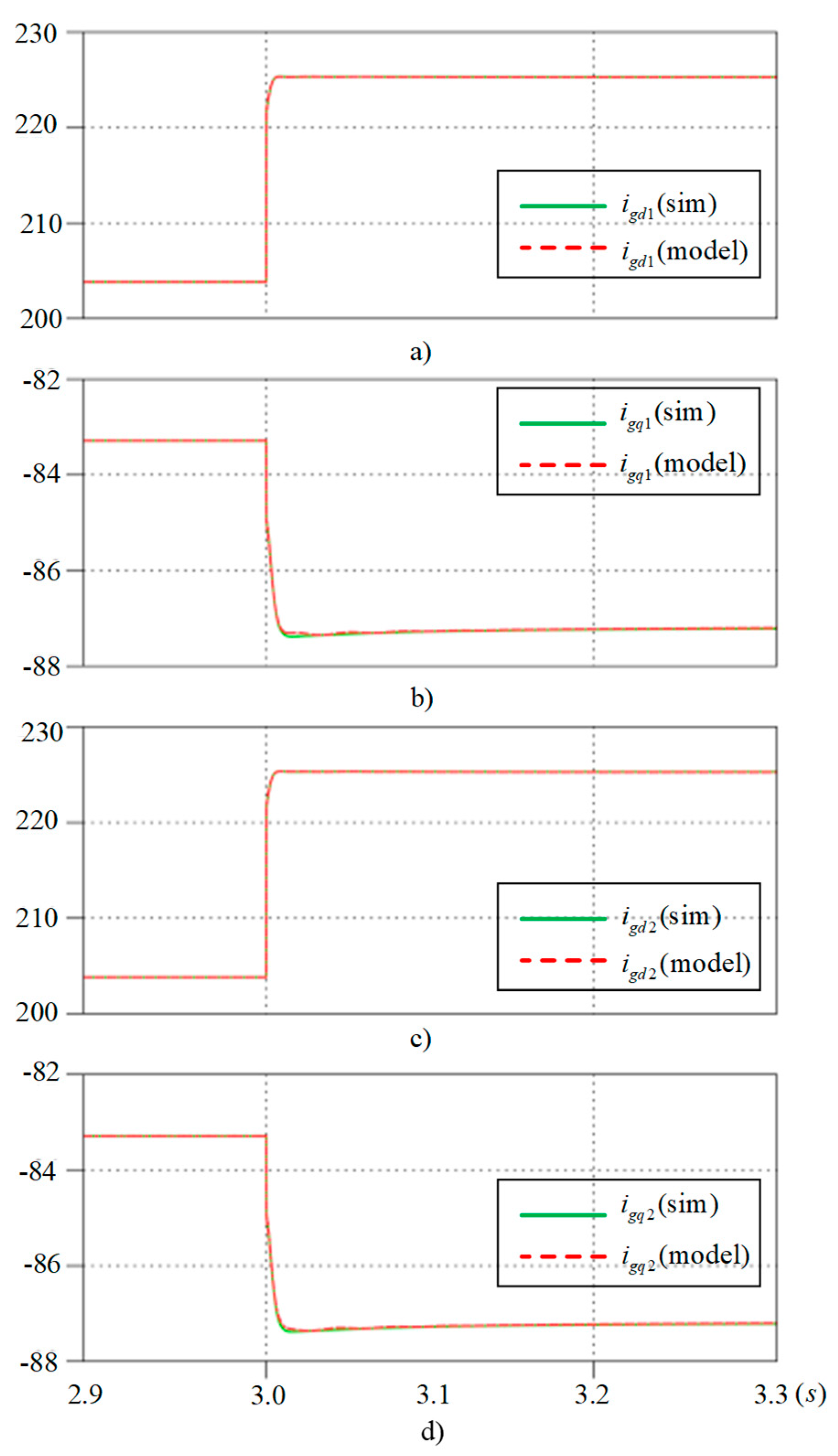
5.1. Validation of Small-Signal Model for GFIs with Proposed Accurate Time Delay Representation in Regard to the dq-Axis

The small-signal model of GFIs with the proposed accurate time delay representation in regard to the dq-axis can be validated by comparing the state-space small-signal model in Equation (47) with real-time simulation results. The bus voltages, ${∆v}_{\mathit{bDQ}1}, {∆v}_{\mathit{bDQ}2}$, and $∆v_{bDQ3}$, are the inputs, and the grid-side currents (${∆i}_{\mathit{gdq}1}, {∆i}_{\mathit{gdq}2}$) are the outputs for the small-signal model of the GFIs.

The island MG parameters are listed in

Table 3. Island microgrid parameters.

Parameter	Value	Parameter	Value
${\omega }_n$	$2\pi 50 \mathrm{rad}/\mathrm{s}$	$r_f$	$1.625 \mathrm{m}\mathsf{\Omega }$
$f_{sw}$	$5 \mathrm{kHz}$	$C_f$	$450 \mathsf{\mu }\mathrm{F}$
$f_{samp}$	$10 \mathrm{kHz}$	$r_{Cf}$	$10 \mathrm{m}\mathsf{\Omega }$
$T_{td}$	$150 \mathsf{\mu }\mathrm{s}$	$L_c$	$247 \mathsf{\mu }\mathrm{H}$
mp	$10\times {10}^{-5}$	$r_c$	$9.2 \mathrm{m}\mathsf{\Omega }$
nq	$10\times {10}^{-5}$	$R_{vir\left(\mathrm{1,2}\right)}$	$10 \mathrm{m}\mathsf{\Omega }$
${\omega }_c$	$2\pi 1 \mathrm{rad}/\mathrm{s}$	$L_{vir\left(\mathrm{1,2}\right)}$	$0.1 \mathrm{mH}$
$K_{bwV}$	175 kHz	$R_{line1}$	$1 \mathrm{m}\mathsf{\Omega }$
$K_{pV}$	0.4948	$L_{line1}$	$1 \mathsf{\mu }\mathrm{H}$
$K_{iV}$	10.9956	$R_{line2}$	$1 \mathrm{m}\mathsf{\Omega }$
$K_{bwC}$	1 kHz	$L_{line2}$	$1 \mathsf{\mu }\mathrm{H}$
$K_{pC}$	0.3393	$R_{load1}$	$0.5 \mathsf{\Omega }$
$K_{iC}$	10.2102	$L_{load1}$	0.5 mH
$L_f$	$54 \mathsf{\mu }\mathrm{H}$	$r_N$	$\mathrm{10,000} \mathsf{\Omega }$

, and the operating point values are given in

Table 4. Operating point values for $m_{p(1,2)}=10\times {10}^{-5}$ and $n_{q(1,2)}=10\times {10}^{-5}$.

Parameter	Value	Parameter	Value
$v_{\mathit{odq}(1,2)}^{\ast }$	[$200 0$]	${\mathrm{V}}_{\mathit{Cqi}}$	$[-5.47 -5.47]$
${\omega }_{\mathit{ni}}$	$[2\mathsf{\pi }\times 50 2\mathsf{\pi }\times 50]$	${\mathrm{I}}_{\mathit{gdi}}$	$[203.82 203.82]$
${\delta }_{\mathit{oi}}$	$[0 0]$	${\mathrm{I}}_{\mathit{gqi}}$	$[-83.28 -83.28]$
${\omega }_{\mathit{oi}}$	$[2\mathsf{\pi }\times 49.22 2\mathsf{\pi }\times 49.22]$	${\mathrm{V}}_{\mathit{bD}}$	$[229.8 229.8]$
${\mathrm{V}}_{\mathit{md}\tau }$	$[239.05 239.05]$	${\mathrm{V}}_{\mathit{bQ}}$	$[-20.27 -20.27]$
${\mathrm{V}}_{\mathit{mq}\tau }$	$\left[8.9605 8.9605\right]$	${\mathrm{I}}_{\mathit{lineD}}$	$[203.81 203.81]$
${\mathrm{I}}_{\mathit{cdi}}$	$[204.62 204.62]$	${\mathrm{I}}_{\mathit{lineQ}}$	$[-83.28 -83.28]$
${\mathbf{I}}_{\mathit{cqi}}$	$[-50.15 -50.15]$	${\mathrm{I}}_{\mathit{loadD}}$	$\left[407.64\right]$
${\mathrm{V}}_{\mathit{Cdi}}$	$[238.04 238.04]$	${\mathrm{I}}_{\mathit{loadQ}}$	$[-166.57]$

. In terms of the steady-state operation, the MG provides power demand in terms of its connected loads at a certain operating point. When a load change occurs, i.e., an increase or decrease in the power demand, a MG needs to adjust its operating point to meet the power demand after a dynamic response. What happens during load changes is a change in the bus voltages, which are the inputs into the small-signal model for GFIs. The response of the small-signal model corresponds to the change in the grid-side currents, ${∆i}_{\mathit{gdq}1}, {∆i}_{\mathit{gdq}2}$, when the change in the bus voltages is taken as the input. When are taken as the initial conditions of the MG and a load change of 5 Ω is introduced into the system at t = 3 s, the simulation and small-signal model responses of the dq-axis grid-side currents are shown in Figure 8. The figure clearly demonstrates that the simulation and the small-signal model of the GFIs, incorporating the proposed accurate time delay representation in regard to the dq-axis, exhibit identical dynamic and steady-state responses to a small change in the system around an operating point. As a result, this confirms the validity of the proposed accurate model for the GFIs through the real-time simulation results.

5.2. Comparison of Conventional Time Delay Modeling and Proposed Accurate Time Delay Representation in Regard to the dq-Axis Accuracy with the Real-Time Simulation Results

In this paper, precise stability analysis of the MG given in Figure 1 is conducted through the use of a small-signal model of the system matrix, A_MG, considering the proposed accurate time delay representation in regard to the dq-axis. It is also important to note that conventional time delay modeling and the proposed time delay representation are systematically compared to each other.

Small-signal stability analysis provides accurate analysis of microgrids in terms of low-frequency and high-frequency modes of the dynamic system, as expressed in the papers [4,26]. In terms of stability, it is a well-known fact that low-frequency modes are largely sensitive to power controllers (active power droop coefficient, m_p, and reactive power droop coefficient, n_q) in droop-controlled microgrids. As the frequency of the modes increases, high-frequency modes are largely sensitive to the outer voltage controller, the inner current controller, and the output filter parameters. Similar to the results obtained in the literature, in this study, the results show that the proposed accurate time delay representation in regard to the dq-axis has a significant effect on the low-frequency modes and, hence, the power controller. That is why the power controller coefficients (m_p and n_q) are expressed as the most critical parameters, and the results are given based on them. Since the most critical parameters for stability are identified as active and reactive power droop coefficients, a comparison between the conventional model and the proposed model is performed for these coefficients with different values using the PLECS 4.8.1 software and a small-signal model is developed in the MATLAB code environment. In this way, it is possible to judge the accuracy of the proposed model in regard to the conventional model by comparing the stability limits for the power controller coefficients. In fact, the limit values for the active m_p and reactive n_q power droop coefficients that ensure stability are revealed.

Firstly, without the virtual impedance model, the conventional and proposed time delay representation based on small-signal stability are compared by means of the relevant eigenvalues to demonstrate the accuracy of the proposed model. Secondly, the virtual impedance effect on small-signal stability is assessed for the proposed time delay representation compared to the conventional model. As a result, the proposed accurate time delay representation validation is presented, and the precise stability of the island MG is systematically validated. The eigenvalues of the system for the nominal operating point are depicted as shown in

Table 5. Eigenvalues of $A_{MG}$ for $m_{p(1,2)}=10\times {10}^{-5}$ and $n_{q(1,2)}=10\times {10}^{-5}$ for the general approach and the proposed accurate model.

General Approach Time Delay Modeling		Proposed Accurate Time Delay Modeling
Eigenvalues	$\mathbf{Real}(\mathit{\lambda }$$)+\mathbf{Im}(\mathit{\lambda }$)i	Eigenvalues	$\mathbf{Real}(\mathit{\lambda }$$)+\mathbf{Im}(\mathit{\lambda }$)i
${\mathsf{\lambda }}_{1,2}$	−30 × 109 ± 309.1i	${\mathsf{\lambda }}_{1,2}$	−30 × 109 ± 309.1i
${\mathsf{\lambda }}_{3,4}$	−33.6 × 106 ± 309.1i	${\mathsf{\lambda }}_{3,4}$	−33.6 × 106 ± 309.1i
${\mathsf{\lambda }}_{5,6}$	−10 × 109 ± 309.1i	${\mathsf{\lambda }}_{5,6}$	−10 × 109 ± 309.1i
${\mathsf{\lambda }}_{7,8}$	−96,471.3 ± 1131.8i	${\mathsf{\lambda }}_{7,8}$	−96,431.95 ± 2364.5i
${\mathsf{\lambda }}_{9,10}$	−96,459.7 ± 1132.6i	${\mathsf{\lambda }}_{9,10}$	−96,420.4 ± 2365.4i
${\mathsf{\lambda }}_{11,12}$	−20,037.2 ± 49,022.93i	${\mathsf{\lambda }}_{11,12}$	−20,307.34 ± 49,274.8i
${\mathsf{\lambda }}_{13,14}$	−19,705.8 ± 48,359.2i	${\mathsf{\lambda }}_{13,14}$	−19,454.7 ± 48,106i
${\mathsf{\lambda }}_{15,16}$	−20,018.2 ± 49,027i	${\mathsf{\lambda }}_{15,16}$	−20,288.53 ± 49,279i
${\mathsf{\lambda }}_{17,18}$	−19,687.4 ± 48,364.7i	${\mathsf{\lambda }}_{17,18}$	−19,436.19 ± 48,111.4i
${\mathsf{\lambda }}_{19,20}$	−1191.3 ± 12,398.1i	${\mathsf{\lambda }}_{19,20}$	−1350.86 ± 12,539i
${\mathsf{\lambda }}_{21,22}$	−1532.3 ± 11,620.1i	${\mathsf{\lambda }}_{21,22}$	−1370.8 ± 11,483.3i
${\mathsf{\lambda }}_{23,24}$	−950.3 ± 12,580.7i	${\mathsf{\lambda }}_{23,24}$	−1105.8 ± 12,711.8i
${\mathsf{\lambda }}_{25,26}$	−1273.7 ± 11,812.3i	${\mathsf{\lambda }}_{25,26}$	−1116.88 ± 11,686.8i
${\mathsf{\lambda }}_{27,28}$	−1082 ± 249.9i	${\mathsf{\lambda }}_{27,28}$	−1109.28 ± 322.6i
${\mathsf{\lambda }}_{29,30}$	−1291.6 ± 189i	${\mathsf{\lambda }}_{29,30}$	−1321.25 ± 374.8i
${\mathsf{\lambda }}_{31,32}$	−420.2 ± 49.6i	${\mathsf{\lambda }}_{31,32}$	−399.22 ± 159.3i
${\mathsf{\lambda }}_{33,34}$	−21.9 ± 123.6i	${\mathsf{\lambda }}_{33,34}$	−2.41 ± 138.5i
${\mathsf{\lambda }}_{35,36}$	−3 ± 21.6i	${\mathsf{\lambda }}_{35,36}$	−32.44 ± 20.5i
${\mathsf{\lambda }}_{37}$	−6.2 + 0.0i	${\mathsf{\lambda }}_{37,38}$	−2.98 ± 21.6i
${\mathsf{\lambda }}_{38}$	−6.45 + 0.0i	${\mathsf{\lambda }}_{39,40}$	−28.23 ± 20.9i
${\mathsf{\lambda }}_{39}$	−8.8 + 0.0i	${\mathsf{\lambda }}_{41}$	−6.2 + 0.0i
${\mathsf{\lambda }}_{40,41}$	−33.7 ± 1.32i	${\mathsf{\lambda }}_{42}$	−6.45 + 0.0i
${\mathsf{\lambda }}_{42,43}$	−33.48 ± 0.024i	${\mathsf{\lambda }}_{43,44}$	−17.38 ± 4.29i
${\mathsf{\lambda }}_{44,45}$	−21.68 ± 0.04i	${\mathsf{\lambda }}_{45,46}$	−17.05 ± 4.47i
${\mathsf{\lambda }}_{46,47}$	−21.34 ± 0.99i	${\mathsf{\lambda }}_{47}$	−8.75 + 0.0i
${\mathsf{\lambda }}_{48}$	0.0 + 0.0i	${\mathsf{\lambda }}_{48}$	0.0 + 0.0i

for both the general approach and modeling, and for the proposed accurate time delay representation. If the real components of all the eigenvalues are negative, i.e., at left half-plane, the system is stable; otherwise, if there exists at least one eigenvalue with a non-negative real component, i.e., at right half-plane, the system is unstable. The imaginary component of eigenvalues represents the frequency modes of the system, including low-frequency modes and high-frequency modes. As can be seen in Table 5, all the eigenvalues have negative real components; therefore, at this operating point, the island MG is said to be stable in regard to both the general approach and the proposed accurate model. However, it is also evident from Table 5 that the eigenvalues in the general approach and proposed accurate model differ from each other, demonstrating that the conventional small-signal model differs from the proposed small-signal model.

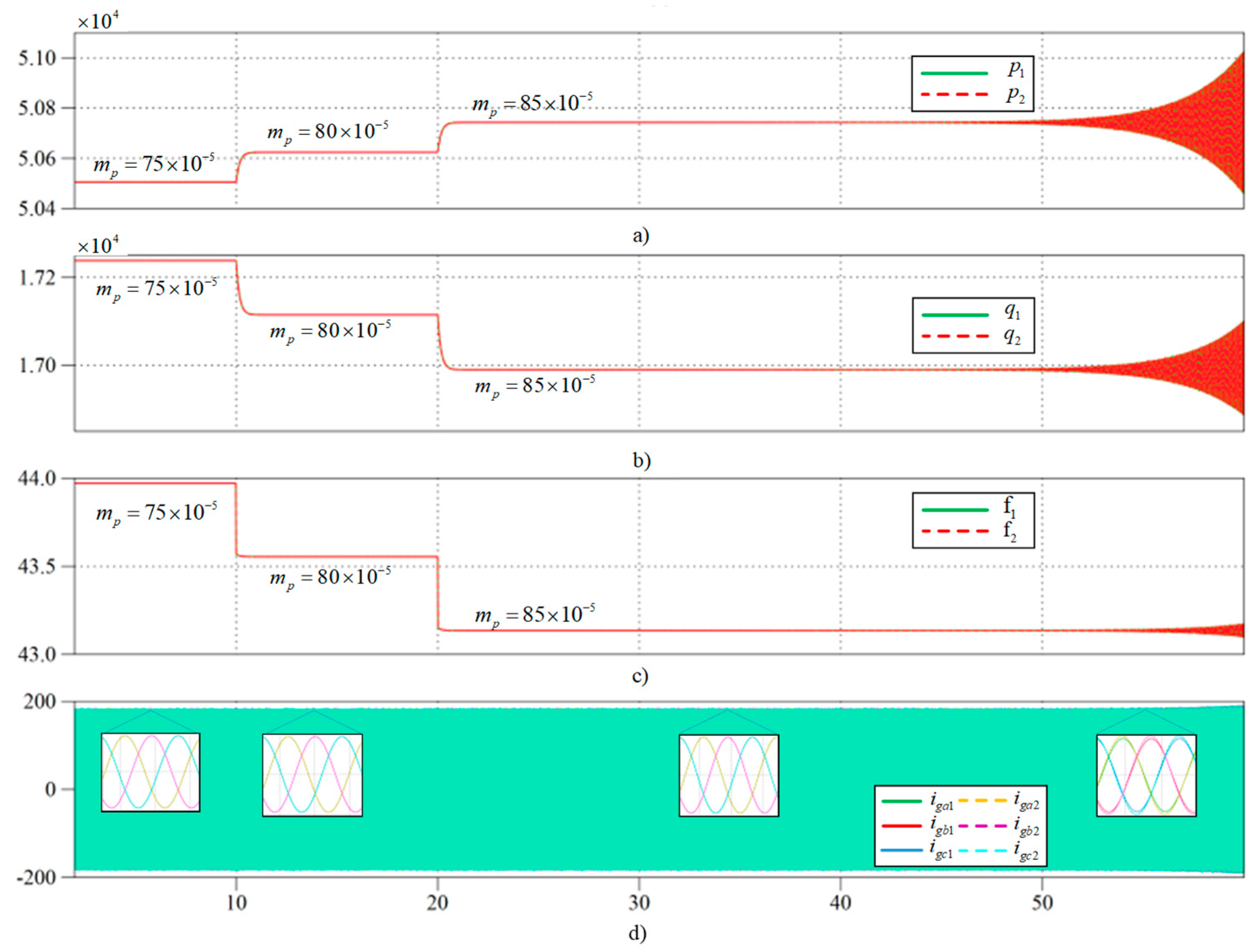
5.2.1. Case 1: Validation Based on Active Power Droop Coefficient

The eigenvalue-based stability analysis for both the system matrix, A_MG, obtained from the general approach time delay model and from the proposed accurate time delay representation is compared in this section through the use of the eigenvalue trajectory and the real-time simulation results. In Figure 9, the eigenvalue trajectory for different values of the active power droop coefficient, m_p, is depicted, while the rest of the system parameters are kept constant as in Table 3. The active power droop coefficient, m_p, is increased from 10 × 10⁻⁵ to 58 × 10⁻⁵ for the general approach model and from 10 × 10⁻⁵ to 75 × 10⁻⁵ for the proposed model, step by step. For all of the values of m_p, the eigenvalues which represent the system modes are obtained, as depicted in Figure 9. In Figure 9, the eigenvalues named as λ_1–18 are not shown, since the real part of the components are far away from the right half of the plane and have a negligible effect on stability. The eigenvalues λ_19–48 are depicted in Figure 9a and a zoomed in view of eigenvalues λ_33–48 is depicted in Figure 9b, which includes the eigenvalues closest to the right half of the plane. As can be seen in Figure 9b, as m_p increases, the eigenvalues λ_33,34 and λ_35–36 move forward to the right half of the plane, namely m_p = 57 × 10⁻⁵ for the general approach model and m_p = 74 × 10⁻⁵ for the proposed model are the limit values in terms of stability. As a result, the theoretical analysis shows that the system is unstable beyond these limit values. It is necessary to note that the eigenvalue trajectories for both models differ from each other and the limit values at the zero-crossing point are not the same. In order to determine which model provides accurate results, a real-time simulation study is carried out for the three different values of m_p, as depicted in Figure 10. These values are m_p = 70 × 10⁻⁵, m_p = 74 × 10⁻⁵, and m_p = 78 × 10⁻⁵. According to the stability analysis, for the first two values of m_p, the island MG is said to be stable, and for the third value of m_p, the system becomes unstable. The simulation results given in Figure 10 reveal that the limit value of m_p for the stability analysis is m_p = 74 × 10⁻⁵, which corresponds to the limit value for the proposed model. However, the limit value for the general approach modeling is much lower than the simulation results. This proves the accuracy of the proposed accurate time delay representation for small-signal analysis, as previously shown in Section 5.1.

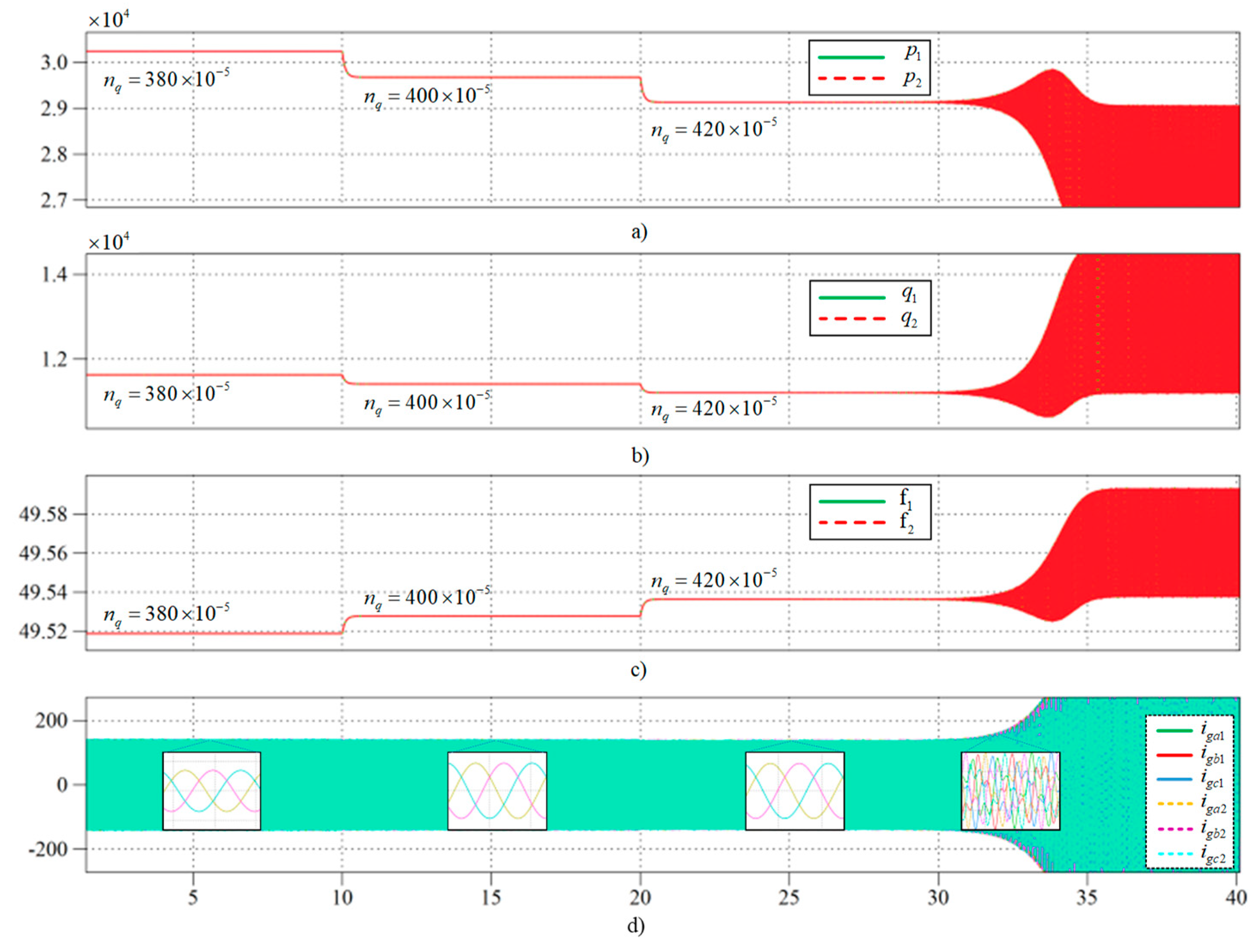
5.2.2. Case 2: Validation Based on Reactive Power Droop Coefficient

The same procedure for the validation based on the reactive power coefficient is carried out, as seen in Figure 9 and Figure 11. In Figure 9c, the eigenvalue trajectory for the different values of the reactive power droop coefficient, n_q, is depicted, while the rest of the system parameters are kept constant, as in Table 3. The reactive power droop coefficient, n_q, is increased from 10 × 10⁻⁵ to 230 × 10⁻⁵ for the general approach model and from 10 × 10⁻⁵ to 35 × 10⁻⁵ for the proposed model, step by step. In Figure 9c, the eigenvalues named as λ_1–18 are not shown, since the real part of the components are far away from the right half of the plane and have a negligible effect on stability. The eigenvalues λ_19–48 are depicted in Figure 9c and a zoomed in view of eigenvalues λ_33–48 is depicted in Figure 9d, which includes the eigenvalues closest to the right half of the plane. As can be seen in Figure 9d, as n_q increases, the eigenvalues λ_33,34 move forward to the right half of the plane, with n_q = 220 × 10⁻⁵ for the general approach model and n_q = 35 × 10⁻⁵ for the proposed model being the limit values in terms of stability. As a result, the theoretical analysis shows that the system is unstable beyond these limit values. It is necessary to note that the eigenvalue trajectories for both models differ from each other and the limit values at the zero-crossing point are not the same. In order to determine which model provides accurate results, a simulation study is carried out for the three different values of n_q, as depicted in Figure 12. These values are n_q = 20 × 10⁻⁵, n_q = 35 × 10⁻⁵, and n_q = 45 × 10⁻⁵. According to the stability analysis for the first two values of n_q, the island MG is said to be stable, and for the third value of m_p, the system becomes unstable. The simulation results given in Figure 11 reveal that the limit value for stability is n_q = 35 × 10⁻⁵, which corresponds to the limit value for the proposed model. However, the limit value for the general approach modeling is much higher than the simulation results. As a result, the proposed accurate time delay representation incorporated into the small-signal analysis matches the real-time simulation results in regard to achieving a high level of accuracy.

5.3. Virtual Impedance Effect Validation on Small-Signal Stability

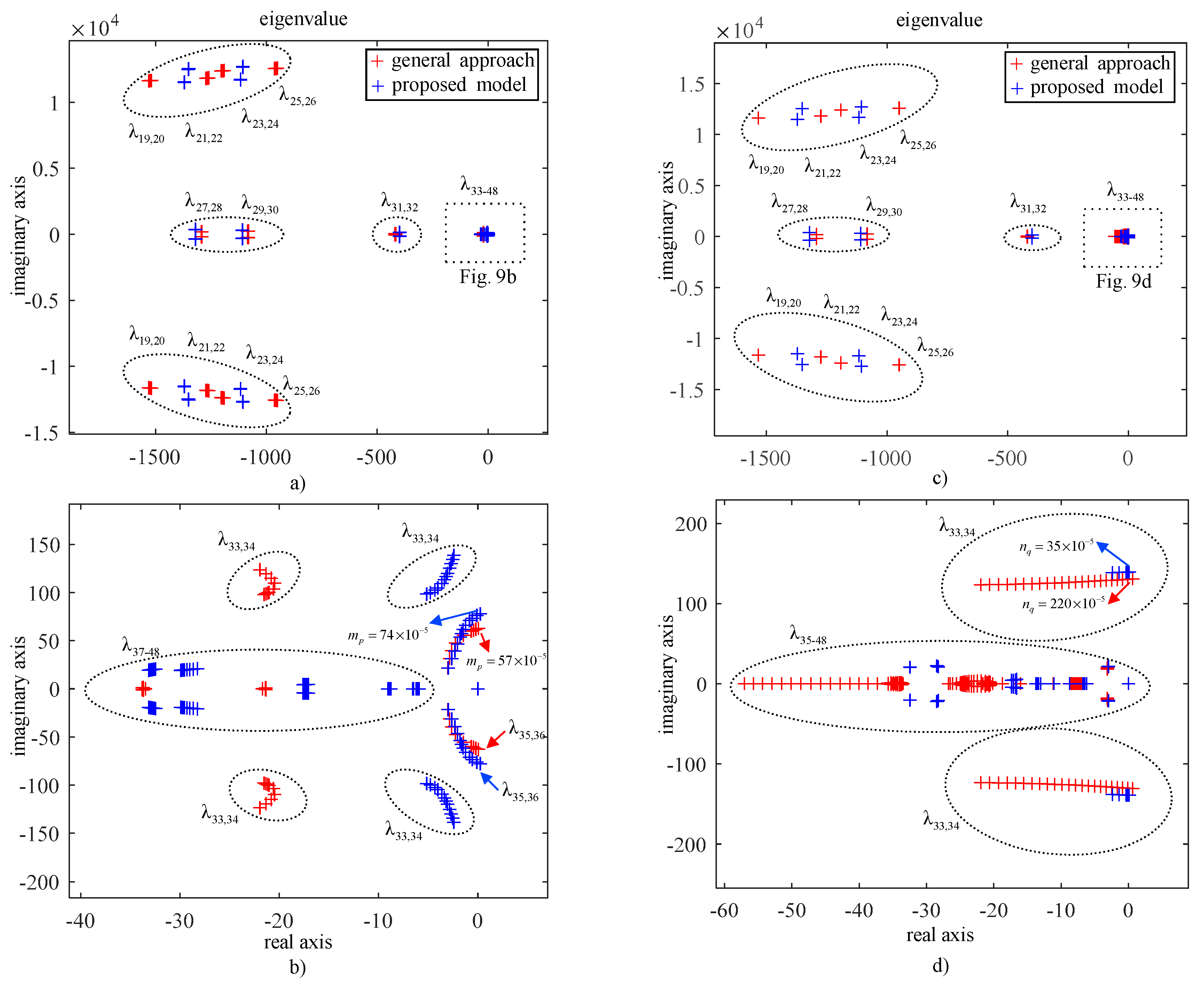
5.3.1. Case 3: Comparison of Virtual Impedance Effect on Stability Based on Eigenvalue Trajectory for Active Power Droop Coefficient

In this case, the virtual impedance effect on the active power droop coefficient is assessed by comparing the proposed small-signal model with the real-time simulation results. As given in Table 3, the virtual impedance is chosen as R_vir = 10 mΩ and L_vir = 0.1 mH. In Figure 12a,b, the eigenvalue trajectories are given both for the system matrix, A_MG, without the virtual impedance model and with the virtual impedance model, as the active power droop coefficient, m_p, is increased from 10 × 10⁻⁵ to 75 × 10⁻⁵ for the proposed model without virtual impedance and from 10 × 10⁻⁵ to 81 × 10⁻⁵ with the virtual impedance, step by step. The eigenvalues named as λ_1–18 are not shown, since the real part of the components are far away from right half of the plane and have a negligible effect on stability; λ_19–48 are depicted in Figure 12a and the zoomed in view of λ_33–48 is depicted in Figure 12b, which includes the eigenvalues closest to the right half of the plane. As can be seen from Figure 12b, the active power droop coefficient limit values are m_p = 74 × 10⁻⁵ for the system matrix without virtual impedance and m_p = 80 × 10⁻⁵ for the system matrix with virtual impedance. In order to show the validity of the small-signal model with virtual impedance, a simulation study is carried out for the three different values of m_p, as depicted in Figure 13. These values are m_p = 75 × 10⁻⁵, m_p = 80 × 10⁻⁵, and m_p = 85 × 10⁻⁵. According to the stability analysis, for the first two values of m_p, the system is said to be stable, and for the third value of m_p, the system becomes unstable. The simulation results given in Figure 13 reveal that the limit value of m_p in terms of stability is m_p = 80 × 10⁻⁵, which corresponds to the limit value in regard to the theorical result. As a result, the limit value of the active power droop coefficient is increased from m_p = 75 × 10⁻⁵ to m_p = 80 × 10⁻⁵ (an increase of approximately 6%) by adding virtual impedance, and the virtual impedance model validity is confirmed for Case 3, according to which the active power droop coefficient is considered.

5.3.2. Case 4: Comparison of Virtual Impedance Effect on Stability Based on Eigenvalue Trajectory for Reactive Power Droop Coefficient

In this case, the virtual impedance effect on the reactive power droop coefficient is evaluated by comparing the proposed small-signal model with the real-time simulation results. In Figure 12c,d, the eigenvalue trajectories are given both for the system matrix, A_MG, without and with the virtual impedance model, as the reactive power droop coefficient, n_q, is increased from 10 × 10⁻⁵ to 35 × 10⁻⁵ for the proposed model without virtual impedance and from 10 × 10⁻⁵ to 400 × 10⁻⁵ with virtual impedance, step by step. A zoomed in view of λ_33–48 is depicted in Figure 12d, which includes the eigenvalues closest to the right half of the plane. As can be seen in Figure 12d, the reactive power droop coefficient limit value is n_q = 35 × 10⁻⁵ for the system matrix without the virtual impedance model and n_q = 400 × 10⁻⁵ for the system matrix with the virtual impedance model. In order to demonstrate the validity of the small-signal model with virtual impedance, a real-time simulation study is conducted for three different values of n_q, as depicted in Figure 14. These values are n_q = 380 × 10⁻⁵, n_q = 400 × 10⁻⁵, and n_q = 420 × 10⁻⁵. The stability analysis suggests that the system remains stable for the first two values of n_q, while it becomes unstable for the third value of n_q. The simulation results in Figure 14 confirm that the limit value of n_q in terms of stability, n_q = 400 × 10⁻⁵, matches the theoretical result. Consequently, the addition of virtual impedance enhances the limit value of the reactive power droop coefficient from n_q = 35 × 10⁻⁵ to n_q = 400 × 10⁻⁵ (an increase of approximately 1000%) and virtual impedance model validity is confirmed for this case. It is important to highlight that adding virtual impedance has a greater impact on the reactive power droop coefficient limit value compared to the active power droop coefficient, as can be concluded from results for Case 3 and Case 4. A summary of the results for the case studies is given in

Table 6. Summary of the case studies.

	Conventional Approach	Proposed Model	Real-Time Simulation Result	Deviation %
Case 1	mp = 57 × 10−5	mp = 74 × 10−5	mp = 74 × 10−5	22%
Case 2	nq = 220 × 10−5	nq = 35 × 10−5	nq = 35 × 10−5	530%
	Without Virtual Impedance	With Virtual Impedance	Real-Time Simulation Result	Deviation %
Case 3	mp = 74 × 10−5	mp = 80 × 10−5	mp = 80 × 10−5	6%
Case 4	nq = 35 × 10−5	nq = 400 × 10−5	nq = 400 × 10−5	1000%

.

6. Discussion

In the existing literature, small-signal stability analysis has been a powerful tool for predicting the stability of microgrids. Many studies have focused on specific aspects of microgrid dynamics, as well as all the dynamics arising from the control structure and physical topology, such as low-frequency and high-frequency (primary and zero-level control) dynamics, as stated in the introduction section. While reduced-order models provide a good understanding of particular dynamics of system behavior, overall stability prediction requires full-order, high-fidelity modeling of the entire microgrid. For this purpose, a digital control-induced time delay model based on the Padé approximation has been incorporated into small-signal modeling in the literature [46,47,48,49]. However, the conventional time delay modeling approach in regard to the dq-axis lacks an accurate representation of time delay effects.

In this paper, the developed small-signal model offers high-fidelity stability analysis with an accurate representation of digital control-induced time delays, as well as the voltage and current control loop. In terms of the proposed accurate time delay representation in regard to the dq-axis synchronous reference frame, both the Heaviside function H(t − T_dt) that is modeled as the Padé approximation transfer function and the phase shift $-\omega T_{td}$ are considered to derive an accurate time delay representation in regard to the dq-axis for the purpose of small-signal stability analysis, since they have a great effect on the stability of island MGs. On one hand, the proposed time delay representation in regard to the dq-axis yields a model fully based on the dq-axis rotating with ωt, facilitating the development of a small-signal model for island MGs; on the other hand, the voltage and current control loop small-signal models are improved by incorporating ω as a state variable into the linearization process. In terms of GFI operation, since droop control is employed, the frequencies of the GFIs vary as the power demand changes. Therefore, it has a significant effect on the accurate modeling of small-signal stability, since decoupling terms in regard to the voltage and current control loops are based on the angular frequency, ω. The validation and accuracy of the proposed model were tested across four different cases, as presented in Section 5, and compared with the conventional modeling approach. The case studies evaluate the impact of the active power droop coefficient, the reactive power droop coefficient, and virtual impedance on stability.

7. Conclusions

This paper aims to provide precise stability analysis of island microgrids (MGs), with a particular emphasis on grid-forming inverters (GFIs). To achieve this objective, a novel and highly accurate digital control-induced time delay model is introduced for use in small-signal stability analysis in regard to the dq-axis synchronous reference frame, significantly enhancing the precision of the analysis. This model incorporates both the Padé approximation of the Heaviside function and the phase shift to accurately represent time delays, and the voltage and current control loop models were refined by including the angular frequency as a state variable in the linearization process.

The results show that the proposed small-signal model is exactly matched, less than a 5% deviation, to the simulation results, whereas the conventional model exhibits a 22% deviation in regard to the active power droop coefficient limit, and a 530% deviation in regard to the reactive power droop coefficient limit. Furthermore, introducing virtual impedance into the proposed small-signal model significantly enhances the microgrid stability limits, enabling a 6% and 1000% increase in the active and reactive power droop coefficients, respectively.

It is important to highlight that this paper provides a high-fidelity framework for future works by addressing shortcomings and areas beyond the scope of this study, such as: (i) evaluating all the parameters in the MG in terms of their impact on stability using sensitivity and participation factor analysis, (ii) investigating various types of controllers and physical topologies to assess the stability improvement in a comparative manner, (iii) integrating DC-side dynamics and various generation units into small-signal analysis, (iv) incorporating the switching loss effect into small-signal analysis, and (v) further validation through the use of experimental testing of a physical microgrid.

The theoretical and simulation results are an exact matched, demonstrating how the proposed accurate modeling approach achieves a high level of accuracy and fidelity in terms of small-signal stability analysis. As a result, with the proposed accurate small-signal model for island MGs, the assessment of stability is achieved precisely and with high fidelity. The results contribute to the advancement of MG modeling and stability analysis, providing a reliable framework for designing and optimizing MG applications.

References

1. Rocabert, J.; Luna, A.; Blaabjerg, F.; Rodríguez, P. Control of power converters in AC microgrids. IEEE Trans. Power Electron. 2012, 27, 4734–4749. [Google Scholar] [CrossRef]
2. Olivares, D.E.; Mehrizi-Sani, A.; Etemadi, A.H.; Cañizares, C.A.; Iravani, R.; Kazerani, M.; Hajimiragha, A.H.; Gomis-Bellmunt, O.; Saeedifard, M.; Palma-Behnke, R.; et al. Trends in microgrid control. IEEE Trans. Smart Grid 2014, 5, 1905–1919. [Google Scholar] [CrossRef]
3. Parhizi, S.; Lotfi, H.; Khodaei, A.; Bahramirad, S. State of the art in research on microgrids: A review. IEEE Access 2015, 3, 890–925. [Google Scholar] [CrossRef]
4. Pogaku, N.; Prodanović, M.; Green, T.C. Modeling, analysis and testing of autonomous operation of an inverter-based microgrid. IEEE Trans. Power Electron. 2007, 22, 613–625. [Google Scholar] [CrossRef]
5. Atmaca, O.; Karabacak, M. Frequency, Phase, and Magnitude Difference Locked-Loop Based Linear Synchronization Scheme for Islanded Inverters and Microgrids. IEEE Access 2023, 11, 61748–61772. [Google Scholar] [CrossRef]
6. Ahmed, M.; Meegahapola, L.; Vahidnia, A.; Datta, M. Stability and Control Aspects of Microgrid Architectures-A Comprehensive Review. IEEE Access 2020, 8, 144730–144766. [Google Scholar] [CrossRef]
7. Alkahtani, A.A.; Alfalahi, S.T.Y.; Athamneh, A.A.; Al-Shetwi, A.Q.; Mansor, M.B.; Hannan, M.A.; Agelidis, V.G. Power Quality in Microgrids including Supraharmonics: Issues, Standards, and Mitigations. IEEE Access 2020, 8, 127104–127122. [Google Scholar] [CrossRef]
8. Kamel, R.M. New inverter control for balancing standalone micro-grid phase voltages: A review on MG power quality improvement. Renew. Sustain. Energy Rev. 2016, 63, 520–532. [Google Scholar] [CrossRef]
9. Rathnayake, D.B.; Akrami, M.; Phurailatpam, C.; Me, S.P.; Hadavi, S.; Jayasinghe, G.; Zabihi, S.; Bahrani, B. Grid Forming Inverter Modeling, Control, and Applications. IEEE Access 2021, 9, 114781–114807. [Google Scholar] [CrossRef]
10. Memon, A.A.A.; Karimi, M.; Kauhaniemi, K. Evaluation of New Grid Codes for Converter-Based DERs From the Perspective of AC Microgrid Protection. IEEE Access 2022, 10, 127005–127030. [Google Scholar] [CrossRef]
11. Rahman, M.A.; Islam, M.R. Different control schemes of entire microgrid: A brief overview. In Proceedings of the 2016 3rd International Conference on Electrical Engineering and Information Communication Technology (ICEEICT), Dhaka, Bangladesh, 22–24 September 2016; pp. 1–6. [Google Scholar]
12. Guerrero, J.M.; Chandorkar, M.; Lee, T.L.; Loh, P.C. Advanced control architectures for intelligent microgrids—Part I: Decentralized and hierarchical control. IEEE Trans. Ind. Electron. 2013, 60, 1254–1262. [Google Scholar] [CrossRef]
13. Timbus, A.; Member, S.; Liserre, M.; Member, S.; Teodorescu, R.; Member, S.; Rodriguez, P.; Blaabjerg, F. Evaluation of Current Controllers for Distributed Power Generation Systems. IEEE Trans. Power Electron. 2009, 24, 654–664. [Google Scholar] [CrossRef]
14. Han, Y.; Li, H.; Shen, P.; Coelho, E.A.A.; Guerrero, J.M. Review of Active and Reactive Power Sharing Strategies in Hierarchical Controlled Microgrids. IEEE Trans. Power Electron. 2017, 32, 2427–2451. [Google Scholar] [CrossRef]
15. Tayab, U.B.; Roslan, M.A.B.; Hwai, L.J.; Kashif, M. A review of droop control techniques for microgrid. Renew. Sustain. Energy Rev. 2017, 76, 717–727. [Google Scholar] [CrossRef]
16. Hossain, M.A.; Pota, H.R.; Issa, W.; Hossain, M.J. Overview of AC microgrid controls with inverter-interfaced generations. Energies 2017, 10, 1300. [Google Scholar] [CrossRef]
17. Begum, M.; Li, L.; Zhu, J. Distributed control techniques for autonomous AC Microgrid-A brief review. In Proceedings of the 2017 IEEE Region 10 Humanitarian Technology Conference (R10-HTC), Dhaka, Bangladesh, 21–23 December 2017; pp. 357–362. [Google Scholar]
18. Sun, Y.; Hou, X.; Yang, J.; Han, H.; Su, M.; Guerrero, J.M. New Perspectives on Droop Control in AC Microgrid. IEEE Trans. Ind. Electron. 2017, 64, 5741–5745. [Google Scholar] [CrossRef]
19. Majumder, R.; Ghosh, A.; Ledwich, G.; Zare, F. Angle droop versus frequency droop in a voltage source converter based autonomous microgrid. In Proceedings of the 2009 IEEE Power & Energy Society General Meeting, Calgary, AB, Canada, 26–30 July 2009; pp. 1–8. [Google Scholar]
20. Zhong, Q.C. Robust droop controller for accurate proportional load sharing among inverters operated in parallel. IEEE Trans. Ind. Electron. 2013, 60, 1281–1290. [Google Scholar] [CrossRef]
21. Zhong, Q.C.; Zeng, Y. Universal Droop Control of Inverters with Different Types of Output Impedance. IEEE Access 2016, 4, 702–712. [Google Scholar] [CrossRef]
22. Zhong, Q.C.; Weiss, G. Synchronverters: Inverters that mimic synchronous generators. IEEE Trans. Ind. Electron. 2011, 58, 1259–1267. [Google Scholar] [CrossRef]
23. Mahmood, H.; Michaelson, D.; Jiang, J. Accurate reactive power sharing in an islanded microgrid using adaptive virtual impedances. IEEE Trans. Power Electron. 2015, 30, 1605–1617. [Google Scholar] [CrossRef]
24. Yao, W.; Chen, M.; Matas, J.; Guerrero, J.M.; Qian, Z.M. Design and analysis of the droop control method for parallel inverters considering the impact of the complex impedance on the power sharing. IEEE Trans. Ind. Electron. 2011, 58, 576–588. [Google Scholar] [CrossRef]
25. Zheng, Y. Virtual Inertia Emulation in Islanded Microgrids with Energy Storage System; Delft University of Technology: Delft, The Netherlands, 2016. [Google Scholar]
26. Kundur, P. Power System Stability and Control; John Wiley & Sons: Hoboken, NJ, USA, 1994. [Google Scholar]
27. Coelho, E.A.A.; Cortizo, P.C.; Garcia, P.F.D. Small-signal stability for parallel-connected inverters in stand-alone ac supply systems. IEEE Trans. Ind. Appl. 2002, 38, 533–542. [Google Scholar] [CrossRef]
28. Mohamed, Y.A.I.; El-saadany, E.F.; Member, S. Adaptive Decentralized Droop Controller to Preserve Power Sharing Stability of Paralleled Inverters in Distributed Generation Microgrids. IEEE Trans. Power Electron. 2008, 23, 2806–2816. [Google Scholar] [CrossRef]
29. Wei, Z.; Jie, C.; Gong, C. Small signal modeling and analysis of synchronverters. In Proceedings of the 2015 IEEE 2nd International Future Energy Electronics Conference (IFEEC), Taipei, Taiwan, 1–4 November 2015. [Google Scholar]
30. Vemula, N.K.; Parida, S.K. Small Signal Stability Assessment of an Inverter-Based Microgrid with Universal Droop and Internal Model-Based Controllers. In Proceedings of the 2018 IEEE International Conference on Power Electronics, Drives and Energy Systems (PEDES), Chennai, India, 18–21 December 2018. [Google Scholar]
31. Dheer, D.K.; Vijay, A.S.; Kulkarni, O.V.; Doolla, S. Improvement of stability margin of droop-based islanded microgrids by cascading of lead compensators. IEEE Trans. Ind. Appl. 2019, 55, 3241–3251. [Google Scholar] [CrossRef]
32. Wang, S.; Liu, Z.; Liu, J.; Boroyevich, D.; Burgos, R. Small-signal modeling and stability prediction of parallel droop-controlled inverters based on terminal characteristics of individual inverters. IEEE Trans. Power Electron. 2020, 35, 1045–1063. [Google Scholar] [CrossRef]
33. Naderi, M.; Shafiee, Q.; Bevrani, H.; Blaabjerg, F. Low-Frequency Small-Signal Modeling of Interconnected AC Microgrids. IEEE Trans. Power Syst. 2021, 36, 2786–2797. [Google Scholar] [CrossRef]
34. Rasheduzzaman, M.; Mueller, J.A.; Kimball, J.W. Reduced-order small-signal model of microgrid systems. IEEE Trans. Sustain. Energy 2015, 6, 1292–1305. [Google Scholar] [CrossRef]
35. Leitner, S.; Yazdanian, M.; Mehrizi-Sani, A.; Muetze, A. Small-Signal Stability Analysis of an Inverter-Based Microgrid with Internal Model-Based Controllers. IEEE Trans. Smart Grid 2018, 9, 5393–5402. [Google Scholar] [CrossRef]
36. Moon, H.-J.; Kim, Y.-J.; Moon, S.-I. Frequency-Based Decentralized Conservation Voltage Reduction Incorporated Into Voltage-Current Droop Control for an Inverter-Based Islanded Microgrid. IEEE Access 2019, 7, 140542–140552. [Google Scholar] [CrossRef]
37. Pournazarian, B.; Sangrody, R.; Saeedian, M.; Gomis-Bellmunt, O.; Pouresmaeil, E. Enhancing Microgrid Small-Signal Stability and Reactive Power Sharing Using ANFIS-Tuned Virtual Inductances. IEEE Access 2021, 9, 104915–104926. [Google Scholar] [CrossRef]
38. Simpson-Porco, J.W.; Dörfler, F.; Bullo, F. Voltage Stabilization in Microgrids via Quadratic Droop Control. IEEE Trans. Automat. Control 2017, 62, 1239–1253. [Google Scholar] [CrossRef]
39. Radwan, A.A.A.; Mohamed, Y.A.R.I. Modeling, analysis, and stabilization of converter-fed AC microgrids with high penetration of converter-interfaced loads. IEEE Trans. Smart Grid 2012, 3, 1213–1225. [Google Scholar] [CrossRef]
40. Eberlein, S.; Rudion, K. Small-signal stability modelling, sensitivity analysis and optimization of droop controlled inverters in LV microgrids. Int. J. Electr. Power Energy Syst. 2021, 125, 106404. [Google Scholar] [CrossRef]
41. Abdelgabir, H.; Shaheed, M.N.B.; Elrayyah, A.; Sozer, Y. A Complete Small-Signal Modelling and Adaptive Stability Analysis of Nonlinear Droop-Controlled Microgrids. IEEE Trans. Ind. Appl. 2022, 58, 7620–7633. [Google Scholar] [CrossRef]
42. Dağ, B.; Aydemir, M.T. A simplified stability analysis method for LV inverter-based microgrids. J. Mod. Power Syst. Clean Energy 2019, 7, 612–620. [Google Scholar] [CrossRef]
43. Malik, S.M.; Sun, Y.; Ai, X.; Chen, Z.; Wang, K. Small-Signal Analysis of a Hybrid Microgrid with High PV Penetration. IEEE Access 2019, 7, 119631–119643. [Google Scholar] [CrossRef]
44. Huang, L.; Wu, C.; Zhou, D.; Blaabjerg, F. Impact of Virtual Admittance on Small-Signal Stability of Grid-Forming Inverters. In Proceedings of the 2021 6th IEEE Workshop on the Electronic Grid (eGRID), New Orleans, LA, USA, 8–10 November 2021. [Google Scholar]
45. Liu, R.; Ding, L.; Xue, C.; Li, Y. Small-signal modelling and analysis of microgrids with synchronous and virtual synchronous generators. IET Energy Syst. Integr. 2023, 6, 45–61. [Google Scholar] [CrossRef]
46. Wang, Y.; Wang, X.; Chen, Z.; Blaabjerg, F. Small-Signal Stability Analysis of Inverter-Fed Power Systems Using Component Connection Method. IEEE Trans. Smart Grid 2018, 9, 5301–5310. [Google Scholar] [CrossRef]
47. Wang, Y.; Wang, X.; Blaabjerg, F.; Chen, Z. Harmonic instability assessment using state-space modeling and participation analysis in inverter-fed power systems. IEEE Trans. Ind. Electron. 2017, 64, 806–816. [Google Scholar] [CrossRef]
48. Liu, F.; Liu, W.; Wang, H.; Xie, Z.; Yang, S.; Wang, J. Small Signal Modeling and Discontinuous Stable Regions of Grid-connected Inverter Based on Pade Approximation. In Proceedings of the 2021 IEEE 12th Energy Conversion Congress & Exposition-Asia (ECCE-Asia), Singapore, 24–27 May 2021; pp. 1076–1081. [Google Scholar]
49. Vemula, N.K.; Parida, S.K. Impact of time delay on performance and stability of inverter-fed islanded MG utilizing internal model controller. Int. J. Electr. Power Energy Syst. 2023, 146, 108713. [Google Scholar] [CrossRef]
50. Vandoorn, T.L.; De Kooning, J.D.M.; Meersman, B.; Vandevelde, L. Review of primary control strategies for islanded microgrids with power-electronic interfaces. Renew. Sustain. Energy Rev. 2013, 19, 613–628. [Google Scholar] [CrossRef]
51. Akagi, H.; Watanabe, E.H.; Aredes, M. Instantaneous Power Theory and Applications to Power Conditioning; John Wiley & Sons: Hoboken, NJ, USA, 2017. [Google Scholar]
52. Guerrero, J.M.; Vasquez, J.C.; Matas, J.; De Vicuña, L.G.; Castilla, M. Hierarchical control of droop-controlled AC and DC microgrids—A general approach toward standardization. IEEE Trans. Ind. Electron. 2011, 58, 158–172. [Google Scholar] [CrossRef]
53. Zhong, Q.C.; Hornik, T. Control of Power Inverters in Renewable Energy and Smart Grid Integration; John Wiley & Sons: Hoboken, NJ, USA, 2012. [Google Scholar]
54. Ramezani, M.; Li, S.; Sun, Y. DQ-reference-frame based impedance and power control design of islanded parallel voltage source converters for integration of distributed energy resources. Electr. Power Syst. Res. 2019, 168, 67–80. [Google Scholar] [CrossRef]
55. Zmood, D.N.; Holmes, D.G. Stationary frame current regulation of PWM inverters with zero steady-state error. IEEE Trans. Power Electron. 2003, 18, 814–822. [Google Scholar] [CrossRef]
56. Zou, C.; Liu, B.; Duan, S.; Li, R. Stationary frame equivalent model of proportional-integral controller in dq synchronous frame. IEEE Trans. Power Electron. 2014, 29, 4461–4465. [Google Scholar] [CrossRef]
57. Freijedo, F.D.; Vidal, A.; Yepes, A.G.; Guerrero, J.M.; Lopez, O.; Malvar, J.; Doval-Gandoy, J. Tuning of Synchronous-Frame PI Current Controllers in Grid-Connected Converters Operating at a Low Sampling Rate by MIMO Root Locus. IEEE Trans. Ind. Electron. 2015, 62, 5006–5017. [Google Scholar] [CrossRef]
58. De Bosio, F.; Pastorelli, M.; De Souza Ribeiro, L.A.; Freijedo, F.D.; Guerrero, J.M. Effect of state feedback coupling on the transient performance of voltage source inverters with LC filter. In Proceedings of the 2016 18th European Conference on Power Electronics and Applications (EPE’16 ECCE Europe), Karlsruhe, Germany, 5–9 September 2016. [Google Scholar]
Figure 1. (a) Island MG with parallel-connected GFIs and (b) fundamental frequency equivalent of the island MG represented with ideal voltage sources.
Electronics 14 01625 g001
Figure 2. Representation of droop control for inductive output impedance: (a) P~f droop control and (b) Q~vCi droop control.
Electronics 14 01625 g002
Figure 3. Control block diagram of GFIs in island MGs.
Electronics 14 01625 g003
Figure 4. Time delay representation: (a) the conventional approach [46,47], and (b) the proposed accurate time delay representation in regard to the dq-axis.
Electronics 14 01625 g004
Figure 5. (a) Step response and (b) frequency responses of Padé approximation transfer functions for the time delay Ttd = 150 μs with the increased order (Table 2).
Electronics 14 01625 g005
Figure 6. The dq-axis representation of phase shift ω T td .
Electronics 14 01625 g006
Figure 8. Grid-side current comparison for the simulation and small-signal model: (a) d-axis currents for GFI 1, (b) q-axis currents for GFI 1, (c) d-axis currents for GFI 2, and (d) q-axis currents for GFI 2.
Electronics 14 01625 g008
Figure 9. Case 1: (a) eigenvalue trajectory as the active power droop coefficient mp is increased and (b) zoomed in view of Figure 9a. Case 2: (c) eigenvalue trajectory as the reactive power droop coefficient nq is increased and (d) zoomed in view of Figure 9c.
Electronics 14 01625 g009
Figure 10. Case 1: simulation results when increasing the active power droop coefficient mp: (a) active powers p1 and p2, (b) reactive powers q1 and q2, (c) frequencies f1 and f2, and (d) grid-side currents igabc1 and igabc2 for GFIs, respectively.
Electronics 14 01625 g010
Figure 11. Case 2: simulation results for reactive power droop coefficient nq: (a) active powers p1 and p2, (b) reactive powers q1 and q2, (c) frequencies f1 and f2, and (d) grid-side currents igabc1 and igabc2 for GFIs, respectively.
Electronics 14 01625 g011
Figure 12. Case 3: (a) eigenvalue trajectory as active power droop coefficient mp is increased and (b) zoomed in view of Figure 12a. Case 4: (c) eigenvalue trajectory as reactive power droop coefficient nq is increased and (d) zoomed in view of Figure 12c.
Electronics 14 01625 g012
Figure 13. Case 3: simulation results for active power droop coefficient mp: (a) active powers p1 and p2, (b) reactive power q1 and q2, (c) frequencies f1 and f2, and (d) grid side currents igabc1 and igabc2 for GFIs, respectively.
Electronics 14 01625 g013
Figure 14. Case 4: simulation results for reactive power droop coefficient nq: (a) active powers p1 and p2, (b) reactive powers q1 and q2, (c) frequencies f1 and f2 and (d) grid-side currents igabc1 and igabc2 for GFIs, respectively.
Electronics 14 01625 g014