Research on Train Energy Optimization Based on Dynamic Adaptive Hybrid Algorithms

Abstract

To address the challenges of locomotive and track modeling and the poor convergence of intelligent algorithms in train energy optimization, a multi-objective optimization model is proposed. Based on the uniform bar dynamics model, an interval division method for constant slope resistance values is developed to improve the applicability and accuracy of the energy consumption model under complex track conditions. Additionally, dynamic inertia weights and learning factors are introduced into the PSO-SA algorithm to enhance the algorithm’s adaptive adjustment capabilities at different optimization stages, alleviating the conflict between global search and local convergence. The proposed method not only improves the convergence speed of the solution but also optimizes train speed profiles, reducing traction energy consumption and improving punctuality. Simulation studies carried out using the new reference line demonstrated a 19% reduction in average train energy consumption, validating the correctness and feasibility of the proposed method, which shows great potential for applications in the field of automatic energy-saving driving for trains.

1. Introduction

To align with China’s “Dual Carbon Strategy” and reduce railway transportation costs, optimizing train traction energy consumption has become a critical technical challenge in the industry. By the end of 2023, China’s total railway freight volume reached 5.035 billion tons, with a freight turnover of 3646.039 billion ton-kilometers—an increase of 51.47 billion ton-kilometers compared to the previous year. Additionally, the National Railway Administration reported that railway energy consumption in 2023 amounted to 17.527 million tons of standard coal equivalent, marking a 15.2% year-on-year increase, with traction energy consumption accounting for approximately 52% of the total. Consequently, minimizing traction energy consumption while satisfying operational constraints such as punctuality and speed limits has emerged as a prominent academic focus in recent years [1]. Current research primarily revolves around making improvements to train operational control modes [2,3,4,5,6,7,8] and the application of heuristic algorithms in train systems [9,10,11,12,13,14,15,16,17,18,19,20,21,22,23].

For energy-efficient train operation optimization [2], the conventional “three-phase operational mode” (maximum acceleration–cruising–maximum braking) meets punctuality requirements but incurs high traction energy consumption. To address this, Yang et al. [3] proposed a “four-phase operational mode” (traction–cruising–coasting–braking), demonstrating significant energy savings on long straight tracks. However, practical scenarios involving complex gradients and frequent steep slopes limit the effectiveness of this approach. Building on the four-phase framework, Bai et al. [4] introduced gradient potential energy utilization for extended downhill sections. To accommodate undulating terrains, Zhou et al. [5] incorporated multi-phase operations and proposed a “multi-coasting” strategy. Albrecht et al. [6,7] categorized gradients into mild, steep uphill, and steep downhill segments, analyzing optimal driving strategies under sub-maximum speed conditions. Finally, Ying et al. [8] applied the maximum principle to derive energy-efficient control strategies for steep gradient transitions.

The integration of heuristic algorithms into train autonomous driving systems has significantly enhanced punctuality and energy efficiency [9,10,11]. Fernández et al. [12] employed dynamic non-dominated genetic algorithms and particle swarm optimization to improve schedule adherence. Cao et al. [13] further enhanced system efficiency through the secondary optimization of genetic algorithm-derived speed curves and strategic coasting interval selection. Song et al. [14] implemented real-time state control based on offline-optimized speed profiles to ensure operational flexibility. Cao et al. [15] developed a finite-time dual sliding surface guidance method for robust speed tracking. These advancements collectively facilitate energy–time trade-off optimization. To refine results, Zhang et al. [16] integrated differential amplification and novel crowding distance operators into non-dominated sorting genetic algorithms, while Zhu et al. [17] enhanced traction efficiency by hybridizing particle swarm optimization with niche technology. Hasanzadeh et al. [18] proposed a gradient-and-speed-limit-aware optimization model, and Dominguez et al. [19] validated a Pareto-front-based multi-objective particle swarm optimizer against NSGA-II and empirical Pareto frontiers. Yan et al. [20] introduced a moving-horizon trajectory planning model with adaptive weight allocation, enriching trajectory optimization theory. Addressing voltage fluctuations in traditional energy-saving methods [21,22], Tao et al. [23] devised a holistic optimization framework for energy efficiency and voltage stabilization. These contributions provide critical theoretical and technical foundations for autonomous train operation.

Current challenges in train traction optimization include limitations in dynamic modeling for complex gradients and computational inefficiencies in heuristic algorithms. To address these, this study proposes a uniform rod train dynamics model and establishes equivalent gradient resistance interval partitioning. A multi-objective optimization framework is formulated with energy consumption and travel time as objectives, constrained by speed limits and mechanical forces. To mitigate slow convergence and local optima in traditional algorithms, a dynamic adaptive PSO-SA (Particle Swarm Optimization–Simulated Annealing) algorithm is developed to generate optimal speed profiles. Simulations are conducted using operational data from the 45 km Xinzhun Line to validate the proposed methodology.

2. Mathematical Model for Train Optimization

2.1. A Dynamics Model of the Uniform Rod for Trains

This study abstracts the entire train as a uniformly distributed mass rod. When calculating additional track resistance, the resistance contributions from different gradient intervals are computed based on their respective lengths and subsequently summed. The velocity–distance (V-S) and time–distance (T-S) relationships during train operation are derived as follows:

$${\displaystyle \frac{ds}{dt}}=v$$

(1)

$${\displaystyle \frac{dv}{ds}}={\displaystyle \frac{u_t{F}_t-u_b{F}_b-(f_1+f_2)\times M}{M(1+\gamma )}}$$

(2)

In the equations, $s$ is the train running distance (unit: m); $v$ is the train speed (unit: m/s); $t$ is the train running time (unit: s); $M$ is the train mass (unit: t); $\gamma$ is the rotational mass coefficient; F_t is the traction force (unit: kN), $F_b$ is the braking force (unit: kN); $u_t$ and $u_b$ are the control coefficients under traction and braking conditions, $0\le u_t\le 1$, $0\le u_b\le 1$; $f_1$ is the unit mass basic running resistance; and $f_2$ is the unit mass additional resistance (unit: kN).

Based on the established train dynamics model, the traction force F_t and braking force F_b of the train can be calculated using Equation (3). For a given rolling stock configuration, both traction and braking forces are solely dependent on the current speed (v) and notch position (u), where u represents the current notch position and v denotes the current velocity.

$$\left\{\begin{array}{l}{F}_t(v)=f(u,v)\\ F_b(v)=b(u,v)\end{array}\right.$$

(3)

$$f_1(v)=c+bv+a{v}^2$$

(4)

The unit mass basic running resistance can be derived from the Davis equation tailored to specific train types and formations, where $a,b,c$ are the coefficients of the Davis equation. The basic running resistance of the train can be approximated as a quadratic function of velocity.

$$\left\{\begin{array}{l}{f}_2(l)=M\cdot g({\theta }_l+{\displaystyle \frac{600}{R}}+0.00013\times L_l)\\ f_2(L)=f_2(l)\times {\displaystyle \frac{l}{L}}+f_2(L-l)\times {\displaystyle \frac{L-l}{L}}\end{array}\right.$$

(5)

In the equations, $f_2(L)$ denotes the total additional resistance of the train, while $f_2(l)$ denotes the segment-specific additional resistance in subsection l, which includes gradient, curve, and tunnel resistance. The parameters are defined as follows:

• g: gravitational acceleration (unit: $\mathrm{N}\times {\mathrm{Kg}}^{-1}$);
• ${\theta }_l$: gradient at position l;
• R: curve radius at position l (unit: m);
• L: tunnel length (unit: m).

2.2. Energy Consumption–Time Model Based on Discretization of Grade Resistance of Track

Train operation represents a continuous process characterized by frequent gradient variations and complex operational conditions. To achieve precise track modeling, this study adopts the discretized equivalent gradient resistance analysis method illustrated in Figure 1. Based on Equation (5), continuous track segments with identical gradient resistance values are defined as sub-intervals $\Delta s$, enabling the partitioning of the entire line into multiple equivalent gradient resistance sections. By assigning optimal operational modes to distinct intervals, this methodology fully exploits track conditions while facilitating refined calculations of traction energy consumption, running time, and other performance metrics.

It is assumed that the operational interval distance is S, the total actual running time of the train is T, and the subscripts {1,2,3,4} represent the four operational phases of the train: traction, cruising, coasting, and braking. The train’s initial velocity and final velocity are both 0 m/s.

(1)

Under traction mode, assuming constant acceleration within the operational step length Δs, the acceleration, running time, and energy consumption within the interval can be expressed as follows:

$$\left\{\begin{array}{l}{a}_{1,i}=(F_t(v_{1,i})-f_1(v_{1,i})-f_2(l_{1,i}))/M(1+\gamma )\\ v_{1,i+1}=\sqrt{2a_{1,i}\cdot \Delta s+v_{1,i}^2}\\ t_{1,i}={\displaystyle \frac{v_{1,i+1}-v_{1,i}}{a_{1,i}}}\\ E_{1,i}=F_t(v_{1,i})\cdot \Delta s\end{array}\right.$$

(6)

(2)

Under cruising mode, where the traction force equals resistance, the energy consumption within a unit step length Δs corresponds to the work performed against resistance. Consequently, the acceleration, running time, and energy consumption within the interval are defined as follows:

$$\left\{\begin{array}{l}{a}_{2,i}=(F_t(v_{2,i})-f_1(v_{2,i})-f_2(l_{2,i}))/M(1+\gamma )=0\\ v_{2,i+1}=v_{2,i}\\ t_{2,i}={\displaystyle \frac{\Delta s}{v_{2,i}}}\\ E_{2,i}=F_t(v_{2,i})\cdot \Delta s\end{array}\right.$$

(7)

(3)

Under coasting mode, the speed begins to decrease, and both the traction force and energy consumption are reduced to 0. Within the interval, the acceleration and running time are defined as follows:

$$\left\{\begin{array}{l}{a}_{3,i}=(-f_1(v_{3,i})-f_2(l_{3,i}))/M(1+\gamma )\\ v_{3,i+1}=\sqrt{2a_{3,i}\cdot \Delta s+v_{3,i}^2}\\ t_{3,i}={\displaystyle \frac{v_{3,i+1}-v_{3,i}}{a_{3,i}}}\\ E_{3,i}=0\end{array}\right.$$

(8)

(4)

Under braking mode, the train generates regenerative braking energy. Let the feedback efficiency of regenerative braking energy be denoted as $\mu$. The regenerative braking energy $E_{4,i}$ is defined as

$$\left\{\begin{array}{l}{a}_{4,i}=(-F_b(v_{4,i})-f_1(v_{4,i})-f_2(l_{4,i}))/M(1+\gamma )\\ v_{4,i+1}=\sqrt{2a_{4,i}\cdot \Delta s+v_{4,i}^2}\\ t_{4,i}={\displaystyle \frac{v_{4,i+1}-v_{4,i}}{a_{4,i}}}\\ E_{4,i}=\mu \cdot F_b(v_{4,i})\cdot \Delta s\end{array}\right.$$

(9)

In summary, within an interval of distance S, the expressions for train energy consumption and running time are as follows:

$$\left\{\begin{array}{l}E={\displaystyle \sum E_{1,i} +}{\displaystyle \sum E_{2,i} +}{\displaystyle \sum E_{3,i} -}{\displaystyle \sum E_{4,i}}\\ T={\displaystyle \sum t_{1,i}+{\displaystyle \sum t_{2,i} +}{\displaystyle \sum t_{3,i} +}{\displaystyle \sum t_{4,i}}}\end{array}\right.$$

(10)

2.3. Energy Consumption Model

By preprocessing the aforementioned variables and establishing normalized equations, the energy consumption objective function can be expressed as

$${\phi }_E(x)={\displaystyle \frac{E-E_{\min }}{E_{\max }-E_{\min }}}$$

(11)

Among them, $E_{\max }$ and $E_{\min }$ represent the maximum and minimum energy consumption of the train, respectively.

To improve punctuality, a penalty factor $f_t$ is introduced into the optimization objective function. The gradient descent method is employed to penalize delays, with the penalty formulated as

$$f_t=\left\{\begin{array}{lc}0& \hspace{1em}\hspace{1em}\left|T-T_{\mathrm{plan}}\right|\le 15\\ {\displaystyle \frac{1}{2}}{T}_{\mathrm{plan}}& 15\le \left|T-T_{\mathrm{plan}}\right|\le 45\\ T_{\mathrm{plan}}& 45\le \left|T-T_{\mathrm{plan}}\right|\le 60\\ 2T_{\mathrm{plan}}& 60\le \left|T-T_{\mathrm{plan}}\right|\le {\displaystyle \frac{1}{4}}{T}_{\mathrm{plan}}\\ 4T_{\mathrm{plan}}& {\displaystyle \frac{1}{4}}{T}_{\mathrm{plan}}\le \left|T-T_{\mathrm{plan}}\right|\le {\displaystyle \frac{1}{2}}{T}_{\mathrm{plan}}\\ 8T_{\mathrm{plan}}& \hspace{1em}\hspace{1em} \left|T-T_{\mathrm{plan}}\right|\ge {\displaystyle \frac{1}{2}}{T}_{\mathrm{plan}}\end{array}\right.$$

(12)

In the equation, T_plan represents the scheduled time. By incrementally increasing the penalty factor, the algorithm avoids premature convergence and filters out infeasible control sequences. Compared to methods using a single fixed penalty factor, the proposed approach is less prone to becoming trapped in local optima.

Assuming a delay threshold of 60 s, the normalized punctuality equation is defined as

$${\varphi }_T(x)={\displaystyle \frac{f_t}{60}}$$

(13)

By combining Equations (11) and (13), the multi-objective optimization model for the train can be derived as follows:

$$\mathrm{minimize}({\varphi }_E\left(x),{\varphi }_T\right(x\left)\right)$$

(14)

Let the initial velocity of the train be $v(0)$ and the final velocity be $v(s_0)$. The constraints are defined as follows:

$$\left\{\begin{array}{l}v(0)=v(s_0)=0\\ v(x)\le v_{\lim }(x)\end{array}\right.$$

(15)

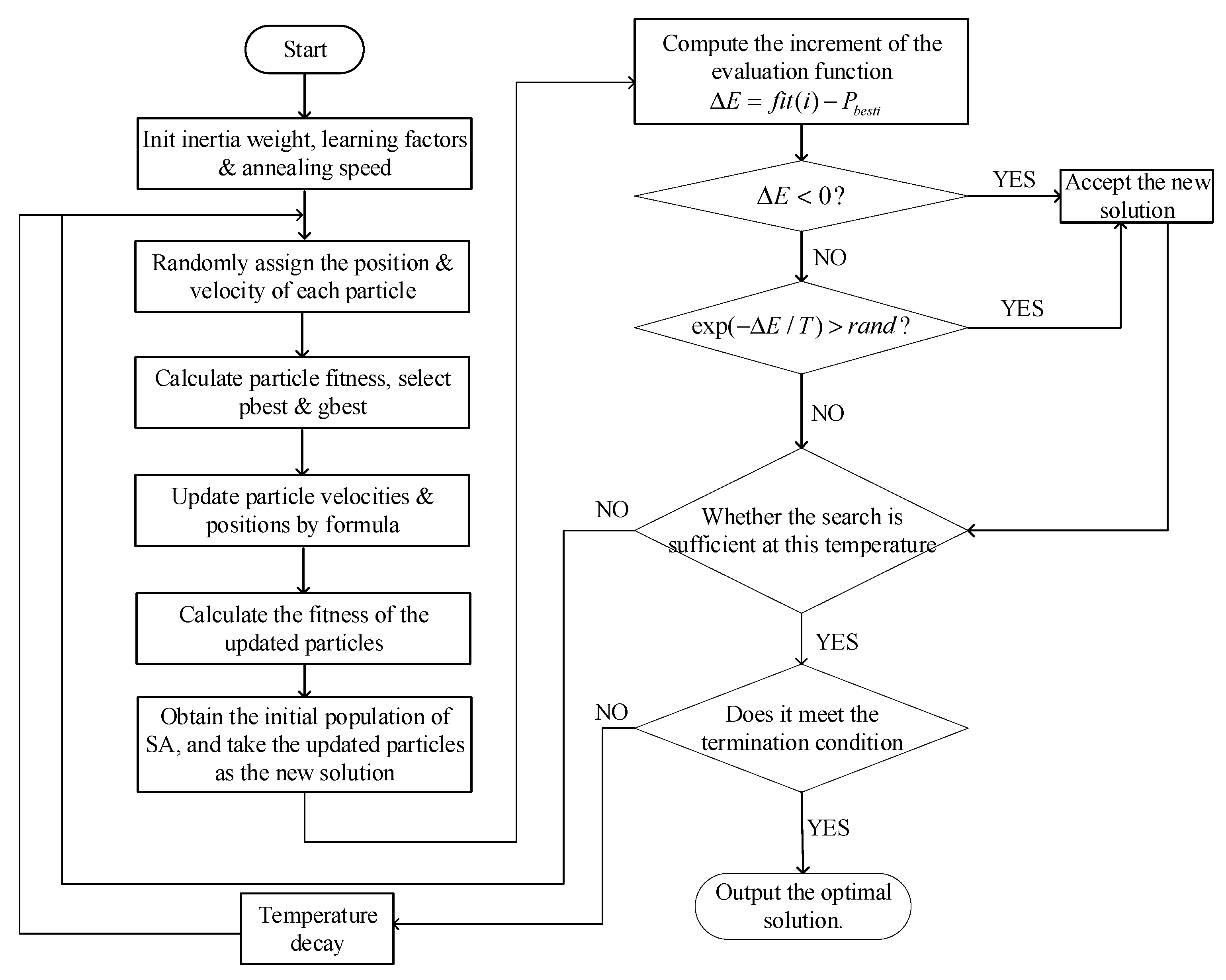
3. Dynamic Adaptive PSO-SA Algorithm for Train Energy Consumption Optimization

Train operation optimization is inherently a multi-objective optimization problem. Studies have demonstrated that using intelligent algorithms is an effective solution to such challenges [24]. This paper proposes a dynamic adaptive PSO-SA multi-objective optimization method, integrating the particle swarm optimization (PSO) and Simulated Annealing (SA) algorithms. The proposed method exhibits fast convergence while mitigating the risk of local optima entrapment.

The PSO algorithm is easy to implement with fewer parameters and demonstrates strong global convergence, yet it is prone to local optima. In contrast, the SA algorithm can escape local optima but faces a trade-off between optimization effectiveness and convergence time due to the computational speed and temporal constraints, often resulting in excessively long convergence periods. By embedding SA into PSO, the hybrid algorithm enhances global search capabilities, maintains population diversity, and improves both convergence speed and optimization precision.

The algorithm adopts a two-layer serial hierarchical structure. The optimization results from PSO serve as the initial solution for SA. After Metropolis criterion-based sampling, SA generates the next-generation population for PSO. The workflow is illustrated in the algorithm flowchart in Figure 2, with the detailed steps outlined below:

Step 1: Initialize the algorithm parameters, including the swarm size N, the position $x_{ij}(t)$ and velocity $v_{ij}(t)$ for each particle, inertia weight $w$, learning factors $c_1$, and $c_2$, cooling rate $\alpha$.

Step 2: Calculate the fitness value for each particle using Equation (16).

$$f={\displaystyle \frac{1}{2}}({\displaystyle \frac{E-E_{\min }}{E_{\max }-E_{\min }}}+{\displaystyle \frac{f_t}{60}})$$

(16)

Step 3: For each particle, compare its fitness value $fit[i]$ with its personal best value $P_{best}(i)$. If $fit[i]<p_{best}(i)$, replace $P_{best}(i)$ with $fit[i]$. Similarly, by comparing $fit[i]$ with $g_{best}$, update the value $g_{best}$ accordingly.

Step 4: Using Equations (17) and (18), update the velocity $v_{ij}$ and position $x_{ij}$ of each particle, and then calculate the corresponding fitness value.

$$\begin{array}{l}{v}_{ij}(t+1)=w\cdot v_{ij}(t)+c_1{r}_1(t)\left[P_{best}(t)-x_{ij}(t)\right]\\ \hspace{1em}\hspace{1em}\hspace{1em}\hspace{1em}\hspace{1em} +c_2{r}_2(t)\left[g_{best}(t)-x_{ij}(t)\right]\end{array}$$

(17)

$$x_{ij}(t+1)=x_{ij}(t)+v_{ij}(t+1)$$

(18)

Step 5: The initial population for SA is directly adopted from the final optimized population obtained in Step 4 of the PSO algorithm. Obtain the initial population of the SA, and let $\Delta E=fit(i)-P_{besti}$.

Step 6: If $\Delta E<0$, accept the current individual as the new solution. Otherwise, accept this individual as the new solution with a probability of $\exp (-\Delta E/T)$.

$$p(1\to 2)=\left\{\begin{array}{ll}1,& \hspace{1em}\hspace{1em}{E}_2<E_1\\ e^{-{\displaystyle \frac{E_2-E_1}{T}}},& \hspace{1em}\hspace{1em}{E}_2\ge E_1\end{array}\right.$$

(19)

Step 7: Carry out the temperature reduction operation: $T=T_0\cdot \alpha$.

Step 8: If the temperature reduction termination condition is satisfied, output the optimal solution.

Given the complexity of train operational environments, the optimization process prioritizes global search capabilities in the initial phase by enhancing particles’ cognitive awareness, thereby mitigating the risk of premature convergence to local optima. During iterations, local search near the global best position $g_{best}$ is emphasized by strengthening inter-particle information exchange and leveraging the influence of the swarm’s optimal position on particle trajectories. To achieve this, we propose adaptively adjusting the inertia weight $w$ and learning factors $c_1,c_2$ in the PSO framework, thereby improving algorithmic performance. The authors of reference [25] selected a hyperbolic tangent curve within the range of [−4, 4] to control the change in the inertia weight coefficient in order to increase the convergence speed of the algorithm and its global search ability.

(1)

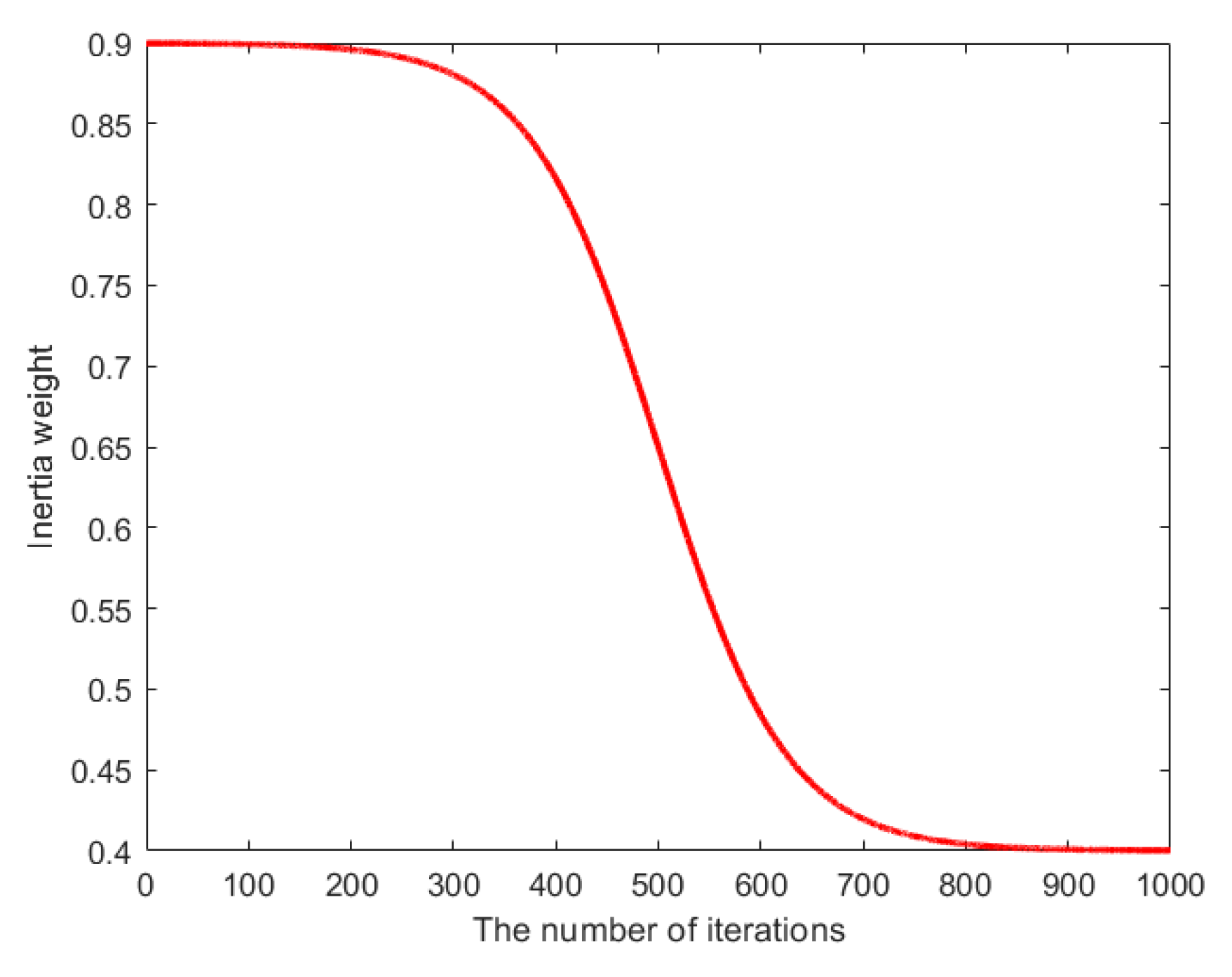
The dynamic adjustment method for the inertia weight is defined as follows:

$$w=(w_{\max }+w_{\min })/2+\tanh (-4+4\times (N-n)/N)(w_{\max }-w_{\min })/2$$

(20)

In the equation, $w_{\max }$ and $w_{\min }$ represent the maximum and minimum inertia weights, set to 0.9 and 0.4, respectively; N denotes the maximum number of iterations; and n denotes the current iteration count. As shown in Figure 3, the inertia weight adjustment curve exhibits three distinct phases. During the initial optimization stage, the inertia weight $w$ remains relatively large and decreases gradually, ensuring that particles explore the global solution space with larger step sizes. In the mid-phase search, the inertia weight decreases rapidly, facilitating a transition from global exploration to localized refinement. Finally, during the late refinement phase, $w$ stabilizes at a smaller value with a slower rate of change, allowing particles to perform fine-grained searches near potential optima. This adaptive strategy enhances the probability of converging to the optimal velocity curve while balancing exploration and exploitation throughout the optimization process.

(2)

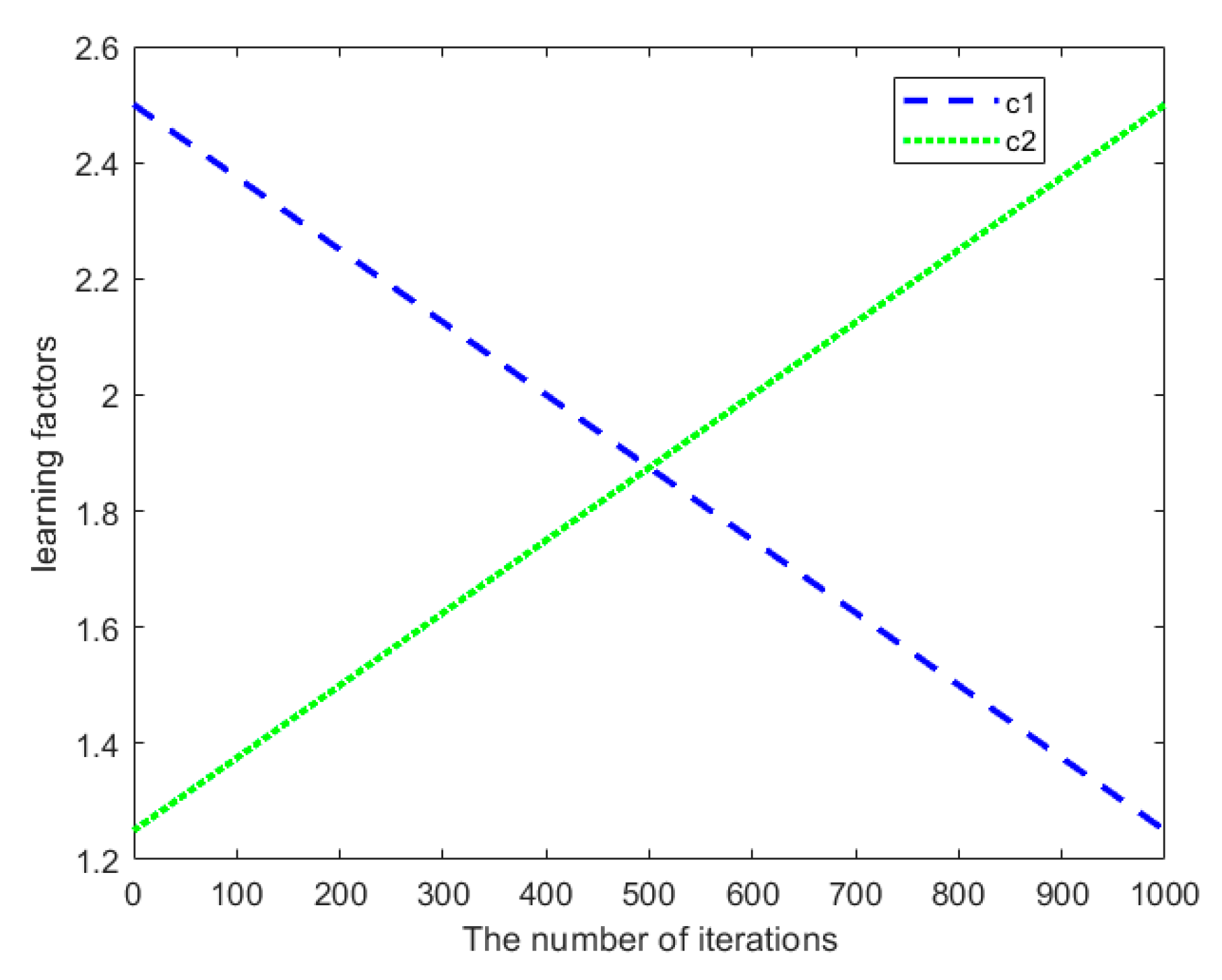
Learning factors c₁ and c₂ regulate the flight of population particles towards the personal optimum and the global optimum. Their adjustment methods are as follows:

$$c_1=c_{1\max }-n(c_{1\max }-c_{1\min })/N$$

(21)

$$c_2=c_{2\min }+n(c_{2\max }-c_{2\min })/N$$

(22)

Among them, $c_{1\max }$ and $c_{1\min }$ are the upper and lower limits of the individual learning factor values, respectively; $c_{2\max }$ and $c_{2min}$ are the upper and lower limits of the group learning factor values, respectively. Here, according to reference [25], we take $c_{1\max }=c_{2\max }=2.5$ and $c_{1\min }=c_{2\min }=1.25$. As shown in Figure 4, $c_1$ decreases linearly from 2.5 to 1.25, while $c_2$ increases linearly from 1.25 to 2.5, which satisfies the spatial ergodicity of particles in the initial search stage. When $c_1<c_2$ and the gap becomes larger, the local search ability also increases accordingly.

4. Case Analysis

4.1. Railway Line Information

A simulation study is conducted by taking the “Sidaoliu–Nalinchuan” section of the Xinzhun freight line as an example, where the total track length is 45 km, characterized by significant variations in gradients, sharp curves, and complex operational conditions. A speed limit of 80 km/h is enforced between 13.621 km and 43.261 km. The line comprises 35 gradients, 24 curves, and seven tunnels. Based on Equation (6), the track can be discretized into 84 segments with equivalent gradient resistance values, where the additional resistance remains constant within each segment. The optimization target is the HXD3 electric locomotive, with its key parameters listed in

Table 1. Structural parameters of HXD3 electric locomotive.

Category	Parameter
Maximum operating speed (km/h)	160
Full-load weight (t)	6000
Maximum tractive force (kN)	580
Maximum braking force (kN)	400
Electric braking power (kW)	7200
Total locomotive efficiency	≥0.85
Basic resistance (kN)	1.20 + 0.0065v + 0.000279v2

.

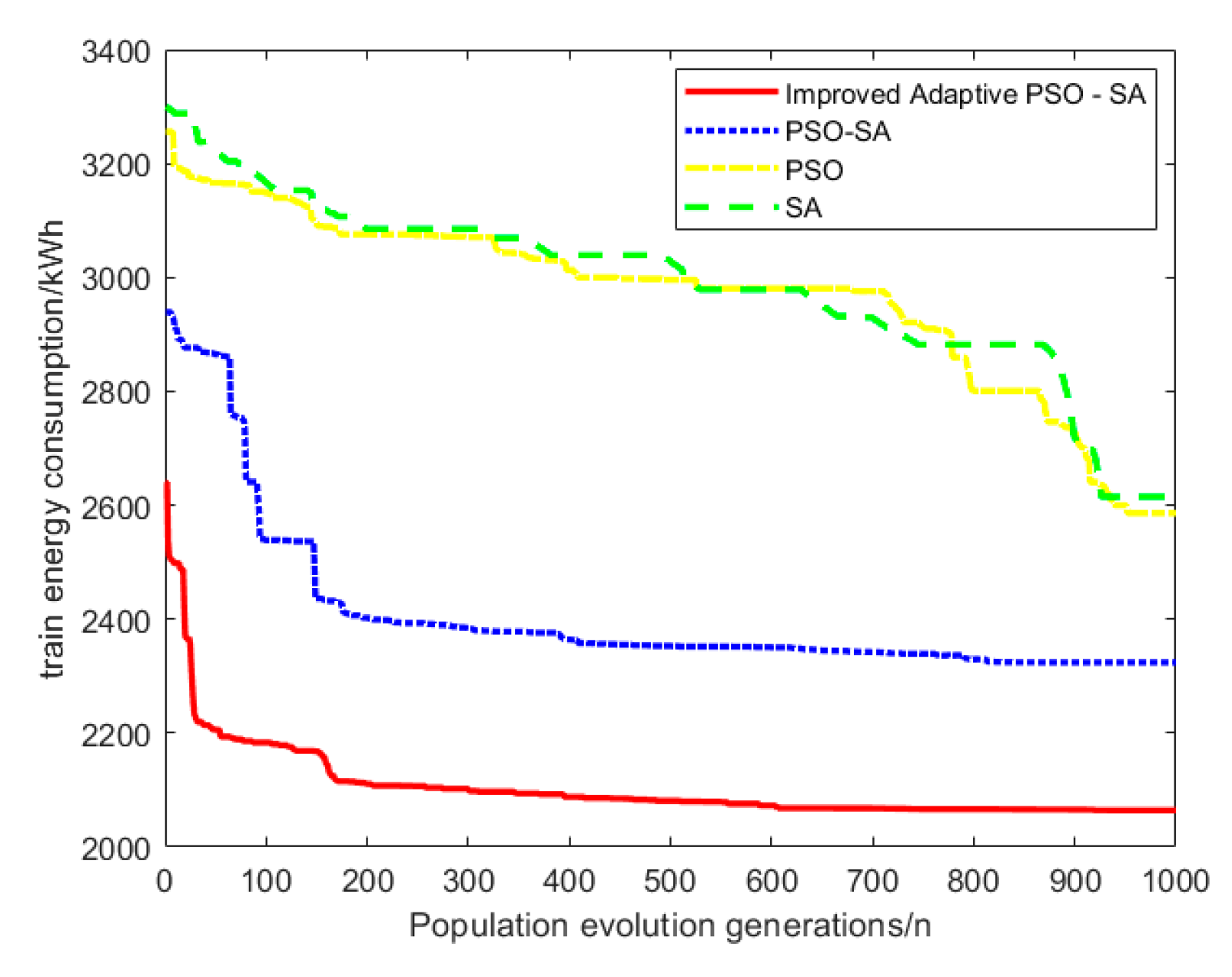
4.2. Evaluation of Dynamic Adaptive PSO-SA Algorithm

Table 2. Comparative analysis results.

Evaluation Indicators	Improved Adaptive PSO-SA Algorithm	PSO-SA	PSO	SA
Average optimal energy consumption (kW·h)	2139.05	2349.48	2595.62	2606.35
Punctuality error (s)	8.22	20.86	31.15	33.48
Average number of iterations	805	836	906	915
Average convergence time (s)	3.09	3.89	4.59	4.46

compares the adaptive PSO-SA algorithm with the PSO-SA, PSO, and SA algorithms regarding optimal energy consumption, the average convergence time, average iteration count, and punctuality error. As shown in Figure 5, which illustrates the relationship between population evolution iterations and the optimal fitness energy consumption of the train, the adaptive PSO-SA algorithm demonstrates superior optimization performance, faster convergence speed, and higher punctuality accuracy compared to the other three algorithms. Figure 6 presents a speed profile comparison before and after optimization. Following the optimized speed curve reduces energy consumption by an average of 20.20%, with an average delay of 8.22 s in punctuality error, which meets the on-time requirements for railway transportation.

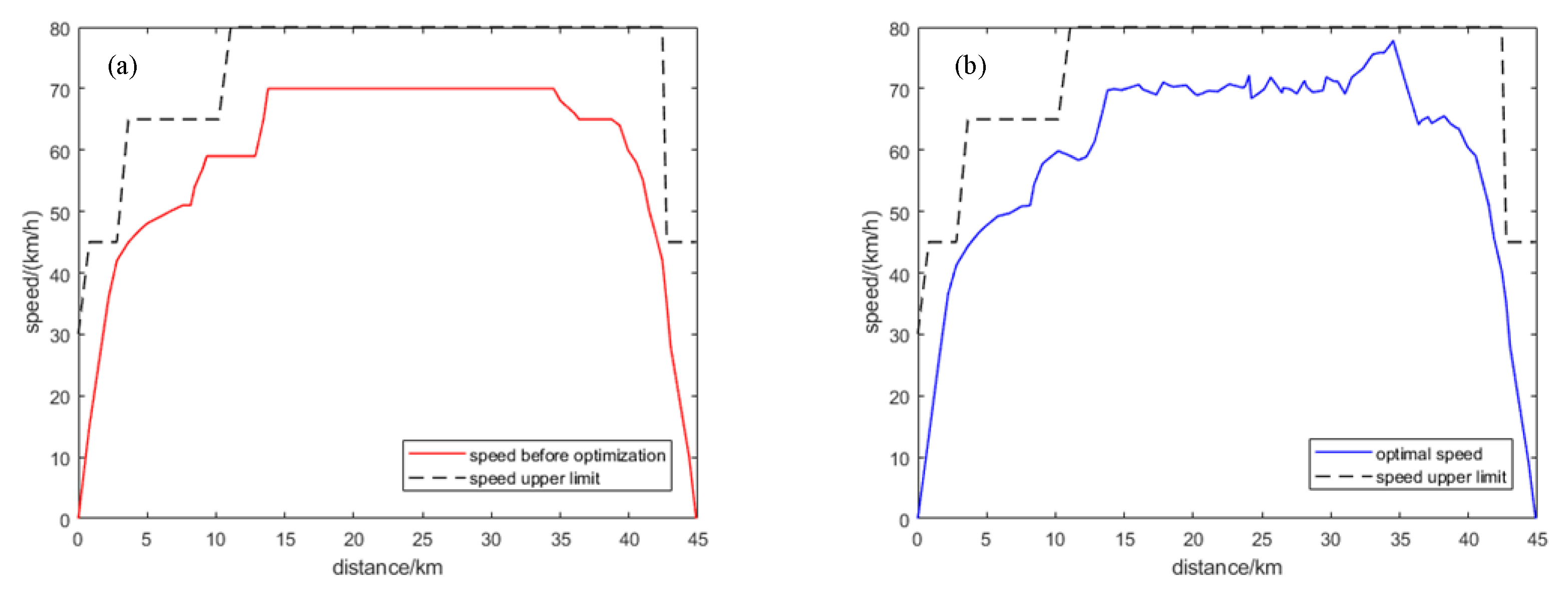
4.3. Comparison of Dynamic Modeling

Table 3. Comparison of kinetic models.

Evaluation Indicators	Single Particle Model	Uniform Rod Model	Multi-Particle Model
Energy consumption (kWh)	2348.24	2125.65	2103.86
Calculation time (t)	2.89	3.13	4.05

presents a performance comparison among the uniform rod model, single-mass point model, and multi-mass point model. The single-mass point model exhibits a faster computation time but incurs higher energy consumption errors. While the uniform rod model demonstrates slightly lower computational accuracy compared to the multi-mass point model, its computational efficiency improved by 22.7%. Additionally, due to the inherent complexity of the multi-mass point model, optimization processes may fail to converge; thus, this study prioritizes the uniform rod model for practical implementation.

This study partitions the track into discrete intervals based on equivalent gradient resistance values. Compared to traditional operational modes, the proposed method fully leverages track conditions by generating adaptive operational mode sequence combinations tailored to each interval. Furthermore, it optimizes the start and end positions of each operational mode to minimize traction energy consumption. The following section details the selection of operational modes for these adaptive intervals, which not only maximizes the utilization of track characteristics but also ensures compliance with punctuality requirements.

Figure 7 illustrates a comparison between train operational modes and section sequences under different control strategies. In traditional control methods, transitions between operational modes occur gradually, failing to fully utilize track conditions and resulting in suboptimal energy-saving performance. In contrast, the optimized control sequence refines the traditional approach by leveraging concave composite gradients to enable potential–kinetic energy conversion, thereby reducing energy consumption. Figure 8 further visualizes the speed profiles across each section, demonstrating the effectiveness of the proposed strategy.

To demonstrate that the optimized operational modes better align with practical conditions, we analyze a track section divided into seven intervals based on equivalent gradient resistance values. Figure 9a depicts the unoptimized operational sequence, where the train follows a conventional four-phase control mode (traction, cruising, coasting, and braking), with cruising, coasting, and braking initiated at positions S_a, S_b, and S_c, respectively. When traversing downhill segment 3, the gradient’s downward force exceeds the running resistance, necessitating partial braking to maintain cruising speed. This prevents full utilization of the gravitational potential energy from the downhill slope. Conversely, on uphill segment 4, partial traction is required to sustain the cruising speed, undermining energy efficiency. Figure 9b illustrates the optimized operational sequence. To fully utilize the gravitational potential energy of downhill segments 3 and 5, coasting mode is implemented between S_a and S_b and between S_c and S_d. To counteract the resistance of uphill segment 4, a brief secondary traction phase is activated between S_b and S_c, ensuring a stable transition to coasting in subsequent segments. Compared to the traditional operational mode, the optimized strategy demonstrates enhanced flexibility and practicality, enabling adaptive adjustments to diverse track conditions and achieving optimal energy-saving outcomes.

5. Conclusions

This study investigated energy-efficient train operation optimization under constraints including speed limits and punctuality requirements and yielded the following conclusions:

(1)

The proposed uniform bar dynamics model resolves the accuracy–efficiency trade-off between single-mass and multi-mass models. By incorporating equivalent slope resistance discretization, it enhances track model precision and, when combined with the uniform bar model, improves the applicability and accuracy of energy consumption models under complex track conditions.

(2)

To solve the optimization model, an adaptive PSO-SA algorithm was developed. Building upon the hybrid PSO-SA framework, it improves inertia weights and learning factors, demonstrating excellent optimization performance, a fast convergence speed, and superior solution distribution characteristics—making it particularly suitable for train traction energy optimization.

(3)

Validation using the Xinzhun Line showed that the proposed method achieves 19% energy savings compared to conventional approaches, demonstrating strong practical applicability and confirming its correctness and effectiveness.

References

1. Feng, X.Y.; Huang, D.Q.; Wang, Q.Y.; Sun, P.F.; He, Q. A review of comprehensive energy saving research for transportation trains. J. China Railw. Soc. 2023, 45, 22–34. [Google Scholar]
2. Zhou, K.; Song, S.; Xue, A.; You, K.; Wu, H. Smart train operation algorithms based on expert knowledge and reinforcement learning. IEEE Trans. Syst. Man Cybern. Syst. 2022, 52, 716–727. [Google Scholar] [CrossRef]
3. Yang, J.; Wu, J.Y.; Wang, B.; Lu, S.F. Research on the optimization algorithm of energy-saving target speed curve for train operation based on heuristic genetic algorithm. J. China Railw. Soc. 2019, 41, 1–8. [Google Scholar]
4. Bai, Y.; Zhou, Y.H.; Qiu, Y.; Jia, J.; Mao, B.H. Energy-saving operation method for metro trains on long and steep downhill tracks. China Railw. Sci. 2018, 39, 108–115. [Google Scholar]
5. Zhou, Y.L.; Ouyang, R.Q.; Lu, R.X.; Cui, J.F.; Wang, Q.; Yang, H. Maneuvering strategy and operation optimization algorithm for low and medium-speed magnetic levitation trains. J. China Railw. Soc. 2024, 1, 451–470. [Google Scholar]
6. Albrecht, A.; Howlett, P.; Pudney, P.; Vu, X.; Zhou, P. The key principles of optimal train control-part 1: Formulation of the model, strategies of optimal type, evolutionary lines, location of optimal switching points. Transp. Res. Part B Methodol. 2016, 94, 482–508. [Google Scholar] [CrossRef]
7. Albrecht, A.; Howlett, P.; Pudney, P.; Vu, X.; Zhou, P. Existence of an optimal strategy, the local energy minimization principle, uniqueness, computational techniques. Transp. Res. Part B Methodol. 2016, 94, 509–538. [Google Scholar] [CrossRef]
8. Ying, P.; Zeng, X.; Song, H.; Shen, T.; Yuan, T. Energy-efficient train operation with steep track and speed limits: A novel Pontryagin’s maximum principle-based approach for adjoint variable discontinuity cases. IET Intell. Transp. Syst. 2021, 15, 1183–1202. [Google Scholar] [CrossRef]
9. Tang, M.N.; Wang, Q.Q. Research on energy-saving optimization of emu trains based on golden ratio genetic algorithm. J. Railw. Sci. Eng. 2020, 17, 16–24. [Google Scholar]
10. Zhang, J.T.; Wu, X.C. Multi-objective optimization of high-speed train ATO operation based on improved mh algorithm. J. Railw. Sci. Eng. 2021, 18, 334–342. [Google Scholar]
11. Zhao, D.S.; Zhao, P.; Yao, X.M.; Yang, Z.; Zhang, B. Optimization of train energy-saving operation strategy based on working condition sequence optimization. J. Transp. Syst. Eng. Inf. Technol. 2024, 24, 157–165. [Google Scholar]
12. Fernández-Rodríguez, A.; Fernández-Cardador, A.; Cucala, A.P. Real time eco-driving of high speed trains by simulation-based dynamic multi-objective optimization. Simul. Model. Pract. Theory 2018, 84, 50–68. [Google Scholar] [CrossRef]
13. Cao, J.F.; Liu, B. Simulation research on energy-efficient operation of high-speed trains based on two-stage optimization. J. Railw. Sci. Eng. 2018, 15, 821–828. [Google Scholar]
14. Song, Y.D.; Song, W.T. A novel dual speed-curve optimization based approach for energy-saving operation of high-speed trains. IEEE Trans. Intell. Transp. Syst. 2016, 17, 1564–1575. [Google Scholar] [CrossRef]
15. Cao, Y.; Wang, Z.C.; Liu, F.; Li, P.; Xie, G. Bio-inspired speed curve optimization and sliding mode tracking control for subway trains. IEEE Trans. Veh. Technol. 2019, 68, 6331–6342. [Google Scholar] [CrossRef]
16. Zhang, H.R.; Jia, L.M.; Wang, L. Generation of energy-saving driving curve sets for high-speed railway trains based on pareto multi-objective optimization. J. China Railw. Soc. 2021, 43, 85–91. [Google Scholar]
17. Zhu, A.H.; Lu, W.; Song, L.M. Research on ATO operation process optimization based on niche particle swarm algorithm. J. Railw. Sci. Eng. 2017, 14, 1998–2004. [Google Scholar]
18. Hasanzadeh, S.; Zarei, S.F.; Najafi, E. A train scheduling for energy optimization: Tehran metro system as a case study. IEEE Trans. Intell. Transp. Syst. 2023, 24, 357–366. [Google Scholar] [CrossRef]
19. Domínguez, M.; Fernández-Cardador, A.; Cucala, A.P.; Gonsalves, T.; Fernández, A. Multi objective particle swarm optimization algorithm for the design of efficient ATO speed profiles in metro lines. Eng. Appl. Artif. Intell. 2014, 29, 43–53. [Google Scholar] [CrossRef]
20. Yan, X.H.; Cai, B.G.; Ning, B.; ShangGuan, W. Moving horizon optimization of dynamic trajectory planning for high-speed train operation. IEEE Trans. Intell. Transp. Syst. 2016, 17, 1258–1270. [Google Scholar] [CrossRef]
21. He, D.Q.; Lu, G.C.; Yang, Y.J. Research on optimization of train energy-saving based on improved chicken swarm optimization. IEEE Access 2019, 7, 121675–121684. [Google Scholar] [CrossRef]
22. Li, G.N.; Or, S.W.; Chan, K.W. Intelligent energy-efficient train trajectory optimization approach based on supervised reinforcement learning for urban rail transits. IEEE Access 2023, 11, 31508–31521. [Google Scholar] [CrossRef]
23. Tao, X.; Wang, Q.; Chen, M.; Sun, P.; Feng, X. Comprehensive optimization of energy consumption and network voltage stability of freight multitrain operation based on amMOPSO algorithm. IEEE Trans. Transp. Electrif. 2024, 10, 4074–4094. [Google Scholar] [CrossRef]
24. Xu, K.; Tu, Y.C.; Xu, W.X.; Wu, S.X. Adaptive multi-intelligence body algorithm optimizing deep networks for intelligent train driving. J. Railw. Sci. Eng. 2022, 19, 2820–2832. [Google Scholar]
25. Yan, Q.M.; Ma, R.Q.; Ma, Y.X.; Wang, J.J. An Adaptive Simulated Annealing Particle Swarm Optimization Algorithm. J. Xidian Univ. 2021, 48, 120–127. [Google Scholar]
Figure 1. Discrete division of train operating zones.
Electronics 14 01588 g001
Figure 2. Algorithm flowchart.
Electronics 14 01588 g002
Figure 3. Adaptive variation in inertia weights.
Electronics 14 01588 g003
Figure 4. Adaptive change in learning factor.
Electronics 14 01588 g004
Figure 5. Comparative analysis of algorithms.
Electronics 14 01588 g005
Figure 6. V-S curves before and after optimization. (a) The V-S curve before optimization. (b) The V-S curve after optimization.
Electronics 14 01588 g006
Figure 7. A comparison of the working condition sequence before and after optimization. (a) The working condition sequence before optimization. (b) The working condition sequence after optimization.
Electronics 14 01588 g007
Figure 8. Velocity profile of each interval.
Electronics 14 01588 g008
Figure 9. Comparison of conventional and optimized manipulation of operating conditions. (a) Sequence of conventional conditions (b) Manipulation of operating conditions after optimization.
Electronics 14 01588 g009