
Joint DOA and Frequency Estimation Method Based on Direct Data Domain

Abstract
1. Introduction
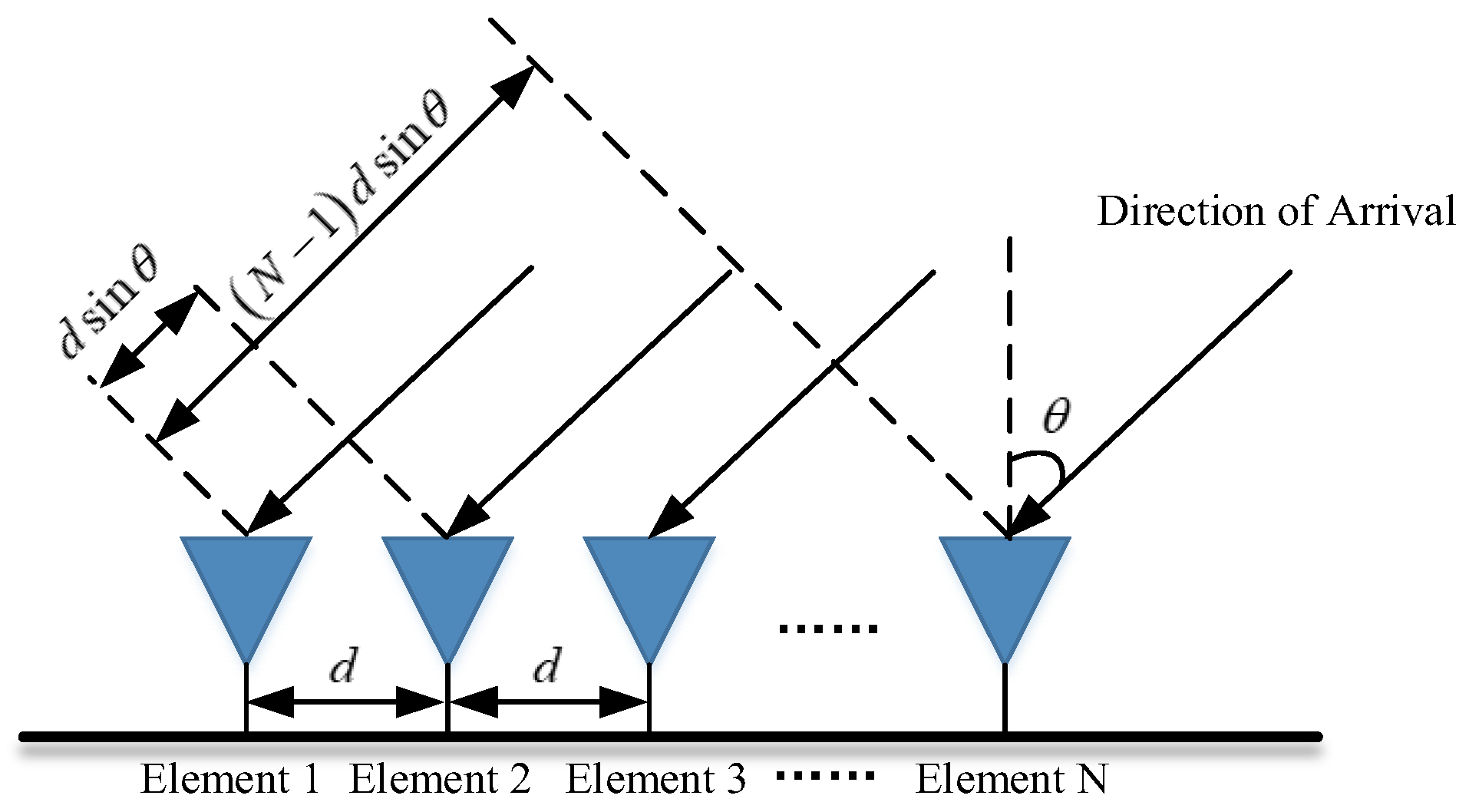
2. Signal Model
3. The Proposed Method
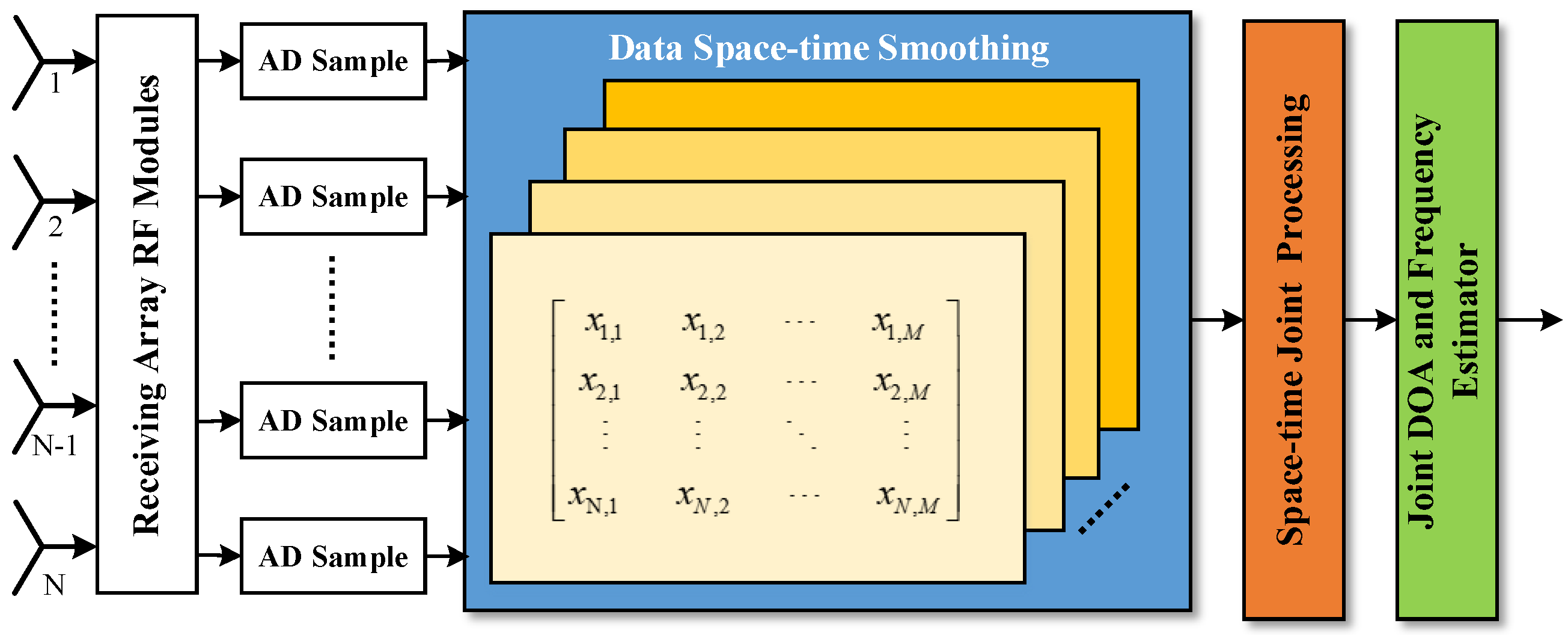
3.1. Design of Digital Receiver
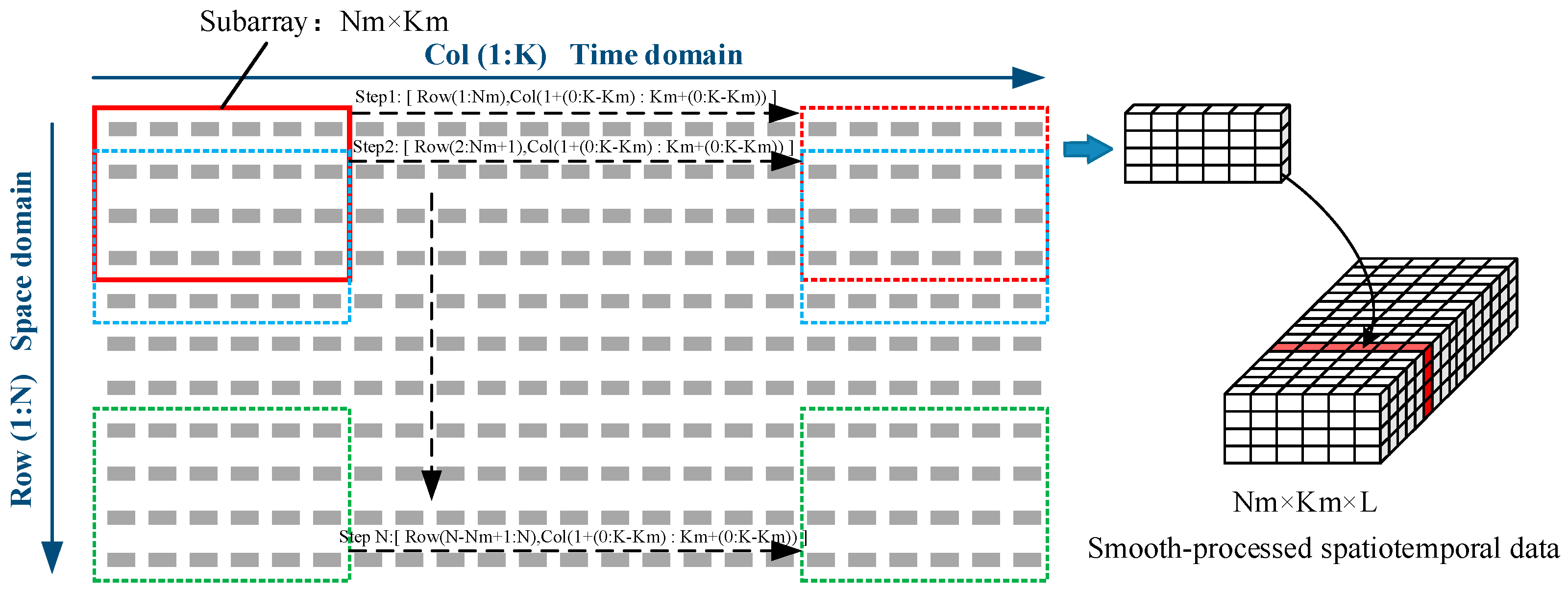
3.2. DDD-JDFE Method
| Algorithm 1. The Proposed Algorithm for Joint DOA and Frequency Estimation | |
| Input: | ; N is the number of antenna elements, K is the number of snapshots; |
| Initialize: | degree; Hz; Aperture: Nm = 12; Km = 24; |
| 1: | |
| 2: | Two-array phase-elimination filtering: ; ; ; |
| 3: | Forward-backward windowing processing: ; |
| 4: | ; |
| 5: | ; |
| 6: | ; |
| 7: | ; |
| 8: | end end |
| 9: | Peak search in two-dimensional matrices: , sN is the number of signals. |
| 10: | |
| 11: | |
| Return: | |
3.3. Array Channel Uncertainty Calibration
3.4. Complexity Analysis
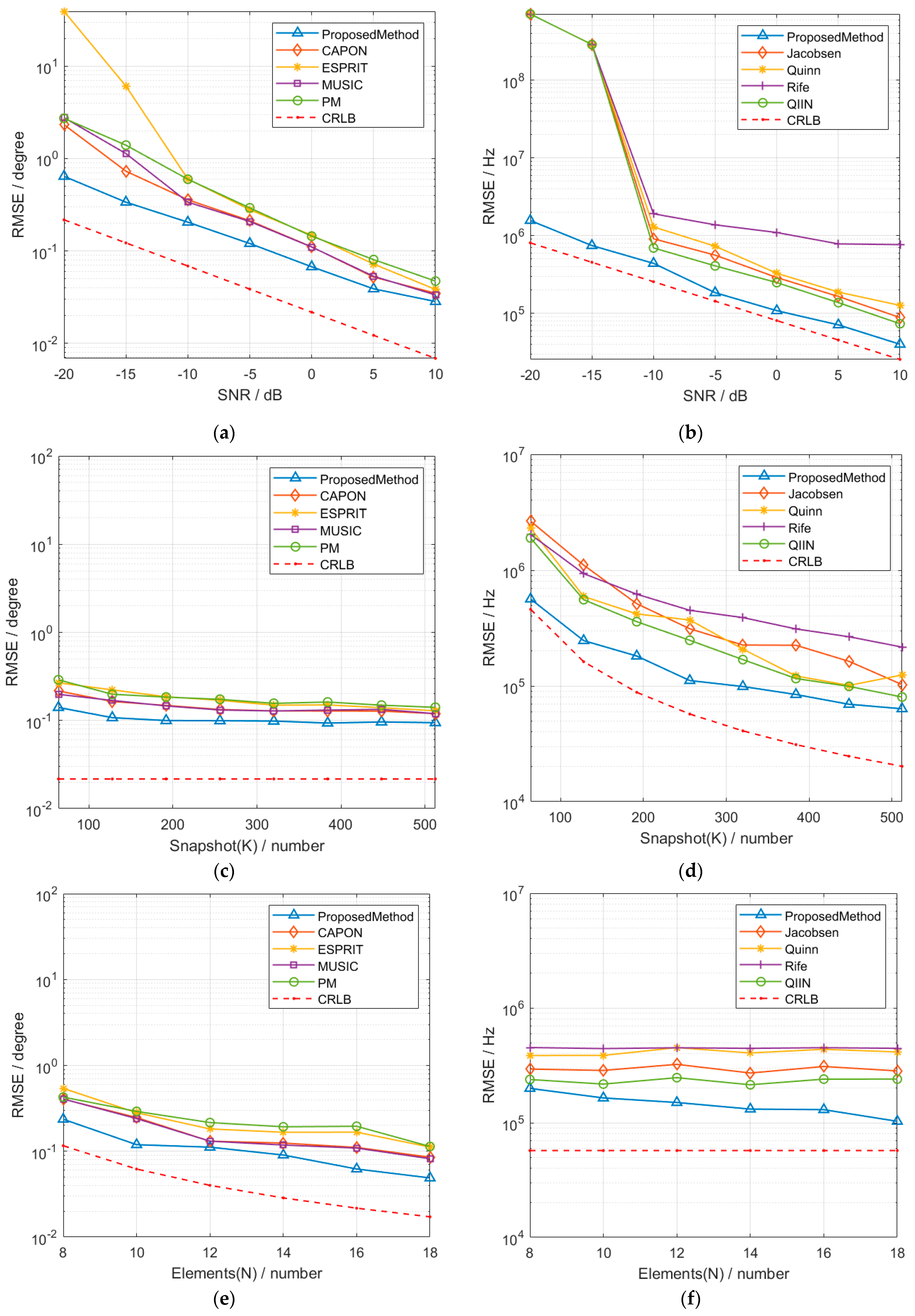
4. Simulation Results
4.1. Simulation Setup
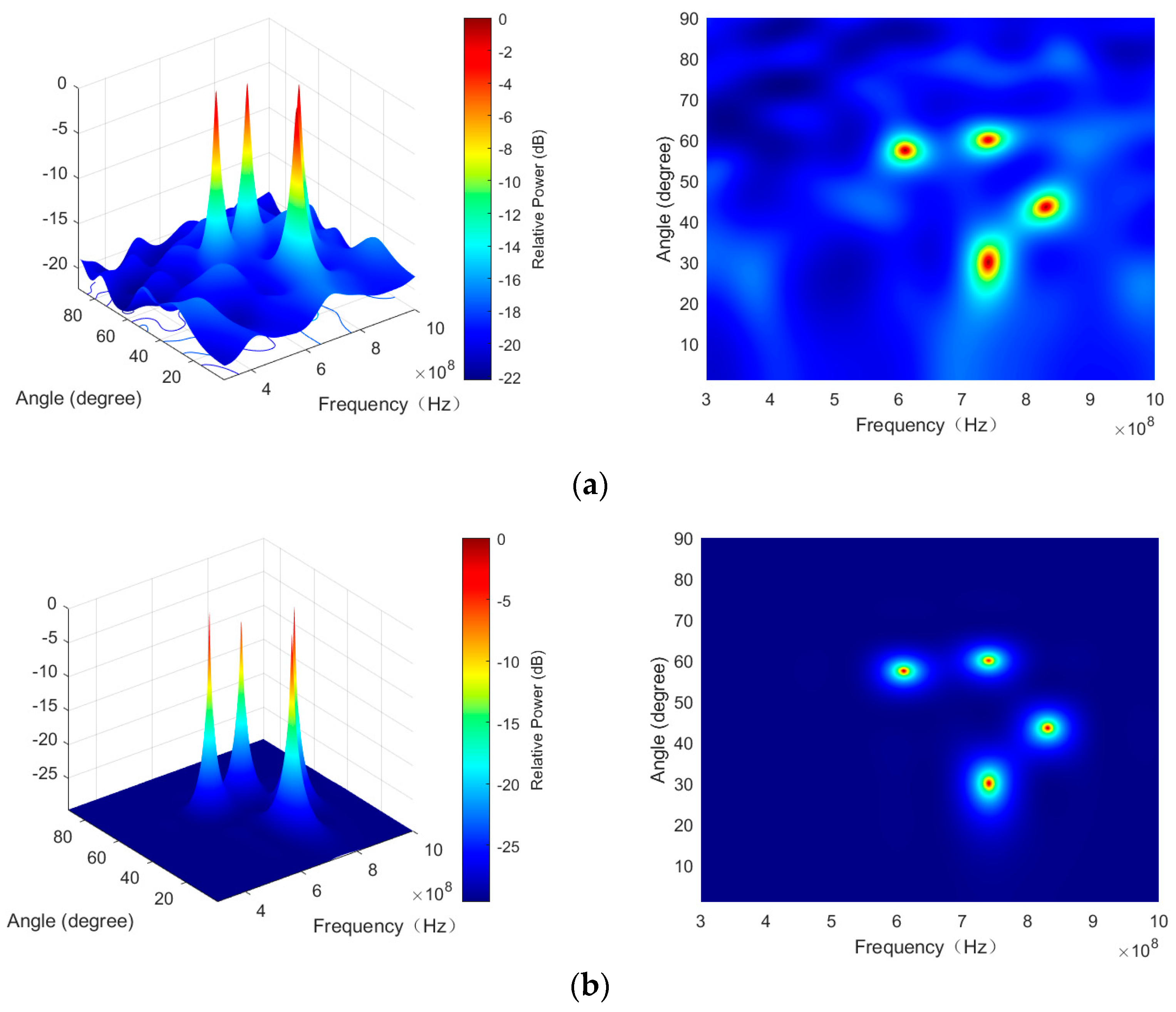
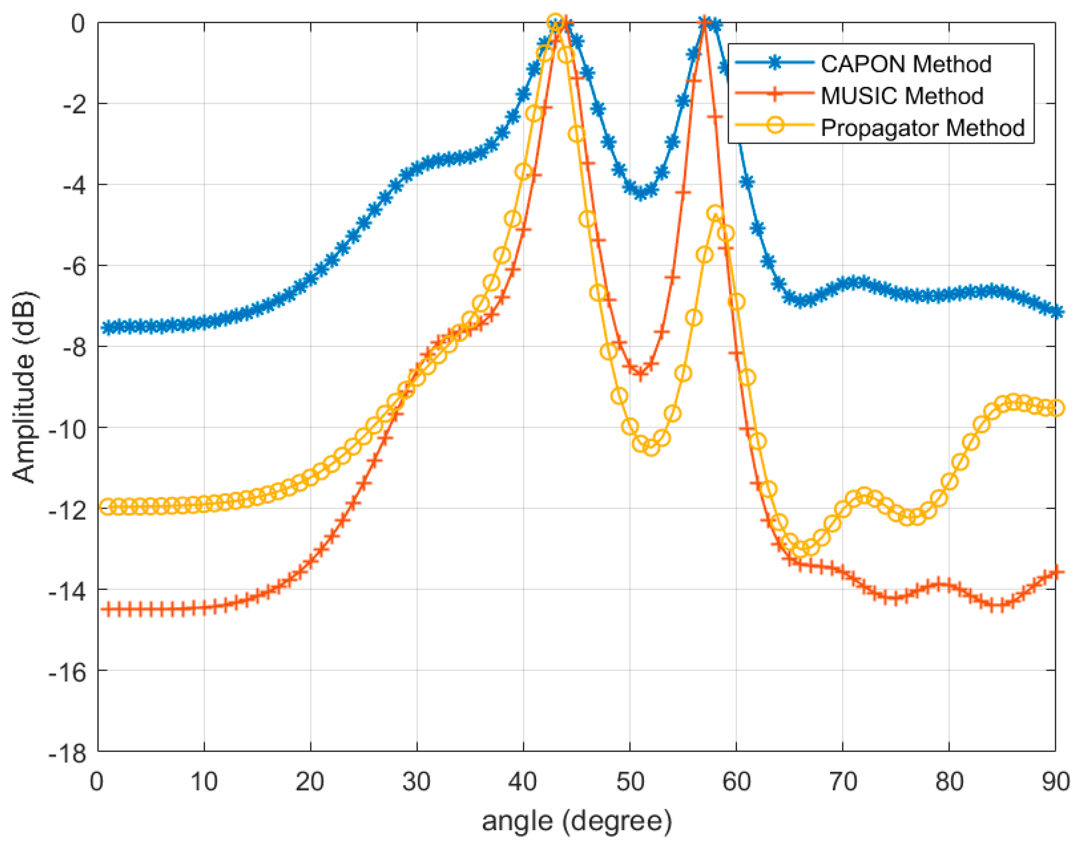
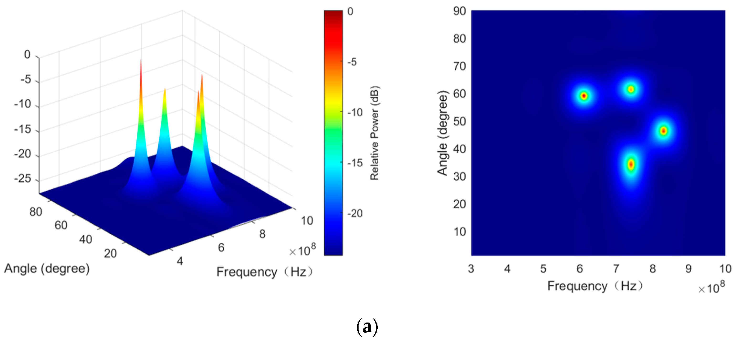
4.2. Comparative Simulation
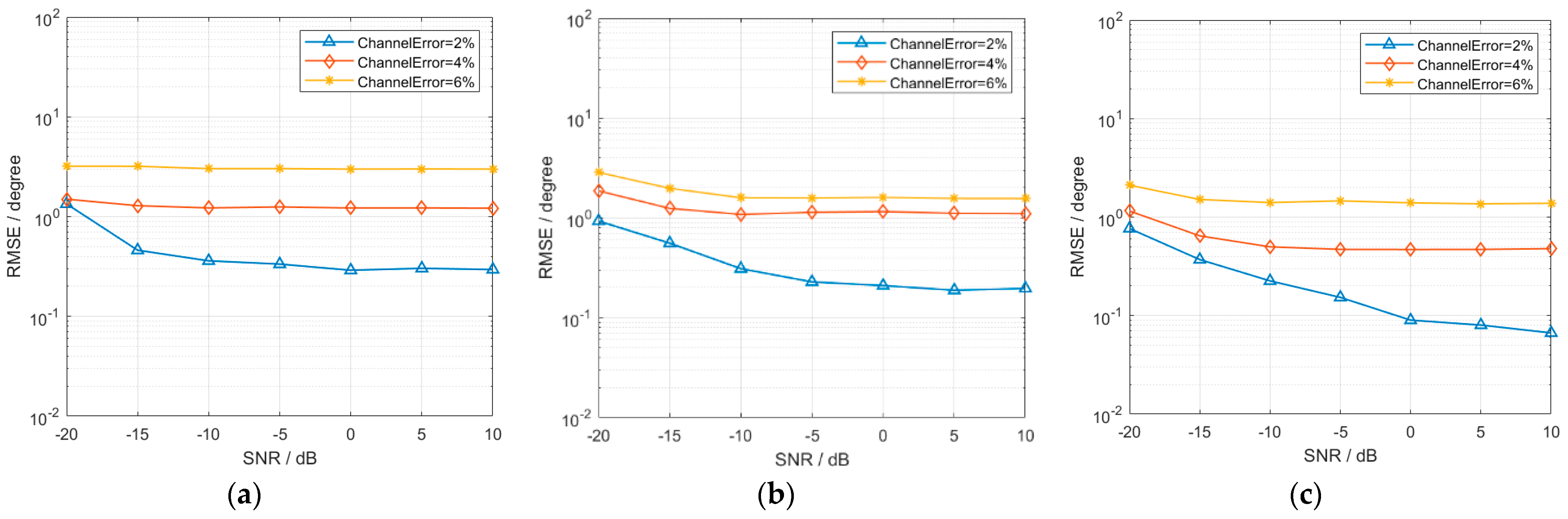
4.3. Array Error Robustness Simulation
4.4. Estimation Performance Comparison Simulation
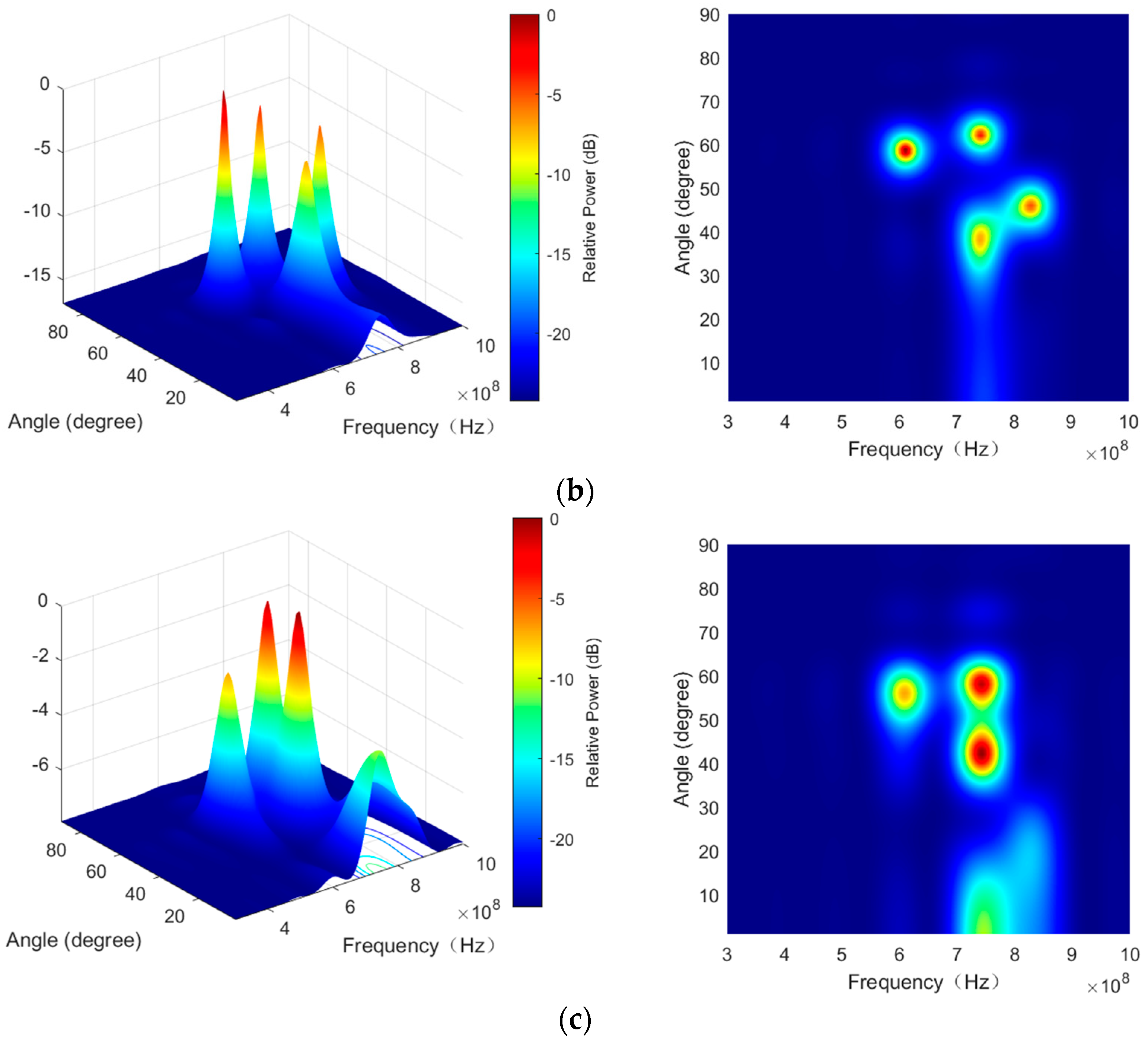
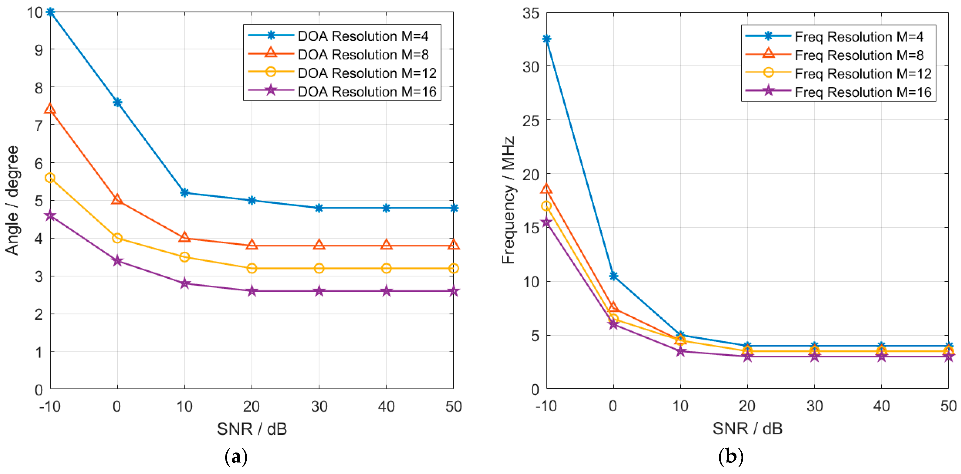
4.5. Multi-Target Resolution Simulation
5. Conclusions
Author Contributions
Funding
Data Availability Statement
Conflicts of Interest
References
- Lemma, A.N.; Van der Veen, A.J.; Deprettere, E. Joint angle-frequency estimation using multi-resolution ESPRIT. In Proceedings of the IEEE International Conference on Acoustics, Speech and Signal Processing, Seattle, WA, USA, 15 May 1998; pp. 1957–1960. [Google Scholar] [CrossRef]
- Lemma, A.N.; Van Der Veen, A.; Deprettere, E.F. Analysis of joint angle-frequency estimation using ESPRIT. IEEE Trans. Signal Process 2003, 51, 1264–1283. [Google Scholar] [CrossRef]
- Xu, L.L.; Zhang, X.F.; Xu, Z.Z. Improved joint direction of arrival and frequency estimation using propagator method. In Proceedings of the 2nd International Conference on Information Science and Engineering, Hangzhou, China, 4–6 December 2010; pp. 2139–2142. [Google Scholar] [CrossRef]
- Lin, J.D.; Fang, W.H.; Wang, Y.Y.; Chen, J.T. FSF MUSIC for joint DOA and frequency estimation and its performance analysis. IEEE Trans. Signal Process. 2006, 54, 4529–4542. [Google Scholar] [CrossRef]
- Stoica, P.; Handel, P.; Soderstrom, T. Study of Capon method for array signal processing. Circuits Syst. Signal Process. 1995, 14, 749–770. [Google Scholar] [CrossRef]
- Rife, D.; Boorstyn, R. Single tone parameter estimation from discrete-time observations. IEEE Trans. Inf. Theory 1974, 20, 591–598. [Google Scholar] [CrossRef]
- Quinn, B.G. Estimating frequency by interpolation using Fourier coefficients. IEEE Trans. Signal Process. 1994, 42, 1264–1268. [Google Scholar] [CrossRef]
- Jacobsen, E.; Kootsookos, P. Fast, accurate frequency estimators. IEEE Signal Process. Mag. 2007, 24, 125–127. [Google Scholar] [CrossRef]
- Jia, P.; Xu, Y.; Zhang, C. A High-Precision Frequency Estimation Algorithm Based on the Q-IIN Algorithm. In Proceedings of the 12th Annual Conference on Satellite Communications 2016, Beijing, China, 3 March 2016; pp. 391–398. [Google Scholar]
- Battaglia, G.M.; Isernia, T.; Palmeri, R.; Morabito, A.F. Synthesis of orbital angular momentum antennas for target localization. Radio Sci. 2023, 58, 1–15. [Google Scholar] [CrossRef]
- Zhu, J.; Yin, T.; Guo, W.; Zhang, B.; Zhou, Z. An Underwater Target Azimuth Trajectory Enhancement Approach in BTR. Appl. Acoust. 2025, 230, 110373. [Google Scholar] [CrossRef]
- Yin, T.; Guo, W.; Zhu, J.; Wu, Y.; Zhang, B.; Zhou, Z. Underwater Broadband Target Detection by Filtering Scanning Azimuths Based on Features of Sub-Band Peaks. IEEE Sens. J. 2025; accepted. [Google Scholar] [CrossRef]
- Zhu, J.; Xie, Z.; Jiang, N.; Song, Y.; Han, S.; Liu, W.; Huang, X. Delay-Doppler Map Shaping through Oversampled Complementary Sets for High Speed Target Detection. Remote Sens. 2024, 16, 2898. [Google Scholar] [CrossRef]
- Sarkar, T.K.; Wang, H.; Park, S.; Adve, R.; Koh, J.; Kim, K.; Zhang, Y.; Wicks, M.; Brown, R. A deterministic least-squares approach to space-time adaptive processing (STAP). IEEE Trans. Antennas Propagat. 2001, 49, 91–103. [Google Scholar] [CrossRef]
- Liao, B.; Liao, G. Method for Array Gain and Phase Uncertainties Calibration Based on ISM and ESPRIT. J. Syst. Eng. Electron. 2009, 20, 223–228. [Google Scholar]
- Chen, D. Array Calibration Technique in DOA Estimation. Ph.D. Thesis, Graduate College, National University of Defense Technology, Changsha, China, 2008. [Google Scholar] [CrossRef]
- Stoica, P.; Nehorai, A. MUSIC, maximum likelihood, and Cramer-Rao bound. IEEE Trans. Acoust. Speech Signal Process. 1989, 37, 720–741. [Google Scholar] [CrossRef]
- Zhou, C.; Haber, F.; Jaggard, D.L. A resolution measure for the MUSIC algorithm and its application to plane wave arrivals contaminated by coherent interference. IEEE Trans. Signal Process. 1991, 39, 454–463. [Google Scholar] [CrossRef]
- Liu, S.; Li, H.; Gou, B. DOA estimation error and resolution loss in linear sensor array. In Proceedings of the 2013 47th Annual Conference on Information Sciences and Systems (CISS), Baltimore, MD, USA, 20–22 March 2013; pp. 1–4. [Google Scholar] [CrossRef]

| No. | Signal Type | Signal Parameters |
|---|---|---|
| 1 | Single-frequency signal | Frequency: 0.74 GHz, Direction: 30° |
| 2 | Chirp Signal | Frequency: 0.62 GH, Band: 20 MHz, Direction: 50° |
| 3 | Single-frequency signal | Frequency: 0.83 GH, Direction: 50° |
| 4 | Single-frequency signal | Frequency: 0.74 GH, Direction: 60° |
| Comparison Content | The Proposed Method | Existing Receivers |
|---|---|---|
| signal gain | Nm × Km = 240 | = 32 |
Disclaimer/Publisher’s Note: The statements, opinions and data contained in all publications are solely those of the individual author(s) and contributor(s) and not of MDPI and/or the editor(s). MDPI and/or the editor(s) disclaim responsibility for any injury to people or property resulting from any ideas, methods, instructions or products referred to in the content. |
© 2025 by the authors. Licensee MDPI, Basel, Switzerland. This article is an open access article distributed under the terms and conditions of the Creative Commons Attribution (CC BY) license (https://creativecommons.org/licenses/by/4.0/).
Share and Cite
Wen, R.; Li, M.; Zheng, L. Joint DOA and Frequency Estimation Method Based on Direct Data Domain. Electronics 2025, 14, 1562. https://doi.org/10.3390/electronics14081562
Wen R, Li M, Zheng L. Joint DOA and Frequency Estimation Method Based on Direct Data Domain. Electronics. 2025; 14(8):1562. https://doi.org/10.3390/electronics14081562
Chicago/Turabian StyleWen, Ronghui, Ming Li, and Lin Zheng. 2025. "Joint DOA and Frequency Estimation Method Based on Direct Data Domain" Electronics 14, no. 8: 1562. https://doi.org/10.3390/electronics14081562
APA StyleWen, R., Li, M., & Zheng, L. (2025). Joint DOA and Frequency Estimation Method Based on Direct Data Domain. Electronics, 14(8), 1562. https://doi.org/10.3390/electronics14081562