A Study on the Electromagnetic Characteristics of Very-Low-Frequency Waves in the Ionosphere Based on FDTD

Abstract

Very-low-frequency electromagnetic waves have low propagation loss, slow attenuation, a stable phase and amplitude in the Earth ionosphere waveguide cavity, and are widely used in VLF communication and navigation, ionospheric heating, global lightning distribution inversion, and other fields. Studying the transmission characteristics of very-low-frequency (VLF) signals in the ionosphere is of great significance in spaceborne VLF communication technology. The existing research on ionospheric transmission characteristics using the finite-difference time domain (FDTD) algorithm is mostly based on high-frequency pulse signals, and the propagation model is relatively rough, resulting in certain calculation errors. To this end, a time-domain finite-difference algorithm model based on a uniaxial anisotropic perfectly matched layer (UPML) boundary in a spherical coordinate system was established, effectively solving the reflection problem existing in PEC boundary. The algorithm was used to numerically calculate the field-strength attenuation of VLF waves in the ionosphere. The simulation results showed that in the VLF frequency band, reducing the frequency is beneficial for electromagnetic waves to penetrate the ionosphere. Although the attenuation trend in the VLF waves is roughly the same during the day and night, the attenuation during the day is significantly greater than that at night, and this was compared and analyzed with traditional algorithms to verify the accuracy of the algorithm.

1. Introduction

Very-low-frequency (VLF) electromagnetic waves refer to electromagnetic waves with a frequency range of 3 kHz to 30 kHz. VLF electromagnetic waves have low propagation loss and slow attenuation, and the signal strength and phase are relatively stable. They are often used in submarine communication and geophysical research [1,2,3,4,5]. In nature, VLF electromagnetic waves can be generated by lightning discharges. The experimental and research results have shown that amplitude-modulated high-frequency electromagnetic waves can be excited to generate ELF/VLF electromagnetic waves by heating the lower ionosphere artificially [5]. The ionosphere is closely related to radio communication, and electromagnetic waves transmitted in it are often affected by changes in the ionosphere [6,7,8,9]. Therefore, it is necessary to study the propagation characteristics of VLF electromagnetic waves in the ionized plasma of the ionosphere for applications such as VLF communication, lightning distribution, and ionospheric heating. The electron density in the ionosphere changes rapidly in the vertical direction and changes slowly in the horizontal direction [4,10,11].

Some scholars have conducted research on the related issues. There are three main calculation methods for electromagnetic-wave propagation in the very-low-frequency field. One is the numerical method, the second is the full-wave method (FWM), and the third is the finite-difference time domain (FDTD) method. The authors of ref. [11] numerically studied the amplitude and spectrum of strong electromagnetic pulses penetrating the ionosphere upwards, providing a reference for the design of electromagnetic pulse protection for low-orbit satellites and other aircraft. When simulating the propagation characteristics of electromagnetic waves in the ionosphere, it is usually necessary to divide the ionosphere into many thin layers. For complex anisotropic media and strong instability in the ionosphere, directly using numerical calculation methods results in insufficient accuracy. The authors of ref. [12] studied the amplitude and spectrum of strong electromagnetic pulses penetrating the ionosphere upwards, providing reference for the design of electromagnetic pulse protection for low-orbit satellites and other aircraft. Reference [13] introduces the current frequency-band distribution of satellite communication and compares it, providing a link budget for S-band satellite communication. The authors of reference [14] used the propagation matrix method to study low-frequency seismic electromagnetic radiation signals. The authors of reference [15] simulated the propagation of electromagnetic pulses in the ionosphere using the FDTD method. The authors of reference [16] applied Z-transform to obtain the iterative relationship between the electric displacement vector D and the electric-field strength E in FDTD derivation, and analyzed the propagation characteristics of high-frequency radar signals in the ionosphere. When simulating the propagation characteristics of electromagnetic waves in the ionosphere, it is usually necessary to divide the ionosphere into many thin layers. With the continuous increase in ionospheric calculation altitude, the time step of FDTD model is limited by the minimum grid size in space, which leads to high computational complexity and memory-space occupation, resulting in error accumulation and inaccurate calculation results [16,17,18]. Therefore, how to quickly and accurately analyze the propagation characteristics of very-low-frequency electromagnetic waves in the ionosphere has become a difficult problem in the fields of computational electromagnetics and radio-wave propagation in recent years [19].

In this paper, a hybrid explicit–implicit time-domain finite difference (HIE-FDTD) method is proposed in the ionosphere. The time-step size of the method is not limited by the size of the spatial grid, so it can overcome the influence of thin-layer structures in the ionosphere on the algorithm’s computing efficiency and has the advantages of high computational accuracy and fast computing speed. The method can realize three-dimensional modeling analysis of VLF electromagnetic-wave propagation in the ionosphere. In addition, it can also provide an important numerical analysis tool for studying the phase and polarization characteristics of VLF electromagnetic waves propagating in magnetized plasma ionosphere.

2. Formulation

2.1. Ionospheric Parameter Model

Near the ground, the ionosphere is weakly ionized, and the electron density and collision frequency between electrons and neutral ions can be calculated by analytical formulas [20,21]. The physical model of electromagnetic-wave propagation in the ionosphere is shown in Figure 1. However, when the height increases, the degree of ionization increases, the electron density and collision frequency of the ionosphere no longer change regularly, and the ionosphere parameters cannot be expressed by formulas [22,23,24]. The description of ionospheric properties involves many parameters, such as electron density and electron collision frequency. In the low ionospheric exponential model established in this paper, the electron density and collision frequency, which have a great influence on the electromagnetic-wave propagation in the ionosphere, are mainly considered. The electron density and collision frequency of the exponential ionospheric parameter model widely used in the low ionosphere are shown in Equation (1) and Equation (2), respectively.

$$N\left(h\right)=1.43\times {10}^7{e}^{-0.15h^{\prime }}{e}^{(\beta -0.15)(h-h^{\prime })}$$

(1)

$$v\left(h\right)=1.816\times {10}^{11}{\mathrm{e}}^{-0.15h^{\prime }}$$

(2)

where N is the electron density, $\upsilon$ is the collision frequency, h is the altitude above the ground, $h^{\prime }$ is the reference altitude, and $\beta$ is the gradient coefficient. The geomagnetic field is also an important reason for the anisotropy of the ionosphere [5]. In the calculation area of the model, the geomagnetic field remains constant with a strength of about 0.5 gauss, here being ${\beta }_0$ = 50 $\mathsf{\mu }$T, if its direction is about 45 degrees relative to the ground and the direction of electromagnetic-wave propagation, and the sizes of each component are ${\beta }_r={\beta }_0/\sqrt{2}$ and ${\beta }_{\theta }={\beta }_{\varphi }={\beta }_0/2$, respectively.

2.2. Equivalent Ionospheric Current-Density Model

In this paper, the influence of electron density and collision frequency in the ionosphere is introduced into the model in the form of current density. The expression of current density in the model is the same as that of electric-field intensity. The current density is based on the momentum equation for electrons moving through the ionosphere, as follows:

$${\displaystyle \frac{d\overrightarrow{J}}{dt}}+\left({\displaystyle \frac{e}{m}}\right)\overrightarrow{J}\times {\overrightarrow{B}}_0+\nu \overrightarrow{J}={ϵ}_0{\omega }_p^2\overrightarrow{E}$$

(3)

where m is the electron mass, e is the electron charge, v is the electron motion speed, ${\overrightarrow{B}}_0$ is the geomagnetic field strength, and ${\omega }_p$ is the plasma frequency.

In the spherical coordinate system, the current-density equation is expressed in the form of three components $J_r$, $J_{\theta }$ and $J_{\varphi }$. Taking the component $J_r$ as an example, the component of the current-density equation is expanded from the $n-1$/2 moment to the $n+1$/2 moment. The formula also contains the current density in the $\theta$- and $\varphi$- directions, so the three components of the current density are interrelated. By performing a time average on the in $\theta$- and $\varphi$- direction components of the current density, the components are made independent of each other. Similarly, for the differential equations of the other two components in the current-density equation, the same method is used to make the components independent of each other. The result of the expansion $J_r$ of the component is shown as follows.

$${\displaystyle \frac{\partial J_r}{\partial t}}+v{J}_r+{\displaystyle \frac{e}{2m}}\left[B_{\phi }\left(J_{\theta }^{n-l/2}+J_{\theta }^{n+l/2}\right)-B_{\theta }\left(J_{\phi }^{n-l/2}+J_{\phi }^{n+l/2}\right)\right]={\epsilon }_0{\omega }_p^2{E}_r^n$$

(4)

The formula contains a derivative with respect to time, and the discretization error is relatively small only when the time step is small. During transmission in a lossy medium, the energy decay of electromagnetic waves is relatively large, and an exponential difference method is adopted in simulation to improve accuracy. To obtain higher precision, an exponential difference is applied to the above formula, and after rearrangement, an iterative equation for $J_r$ can be obtained.

$$J_r^{n+1/2}=2a/b{J}_r^{n-1/2}+{\omega }_{b\theta }(J_{\phi }^{n-1/2}+J_{\phi }^{n+1/2})+2{\epsilon }_0{\omega }_p^2{E}_r^n-{\omega }_{b\varphi }(J_{\theta }^{n-1/2}+J_{\theta }^{n+1/2})$$

(5)

The coefficients in the equation are

$$a=e^{-\nu \Delta t},b={\displaystyle \frac{1-e^{-\nu \Delta t}}{\nu }},{\omega }_{br}={\displaystyle \frac{e}{m}}{B}_{0r},{\omega }_{b\theta }={\displaystyle \frac{e}{m}}{B}_{0\theta },{\omega }_{b\phi }={\displaystyle \frac{e}{m}}{B}_{0\phi }$$

(6)

For the other two components, using the same method, similar equations can be obtained. Combining the three components together, we obtain the matrix form iterative equation for J, which is shown below. It can be abbreviated as

$$A{\overrightarrow{J}}^{n+1/2}=B{\overrightarrow{J}}^{n-1/2}+b{\epsilon }_0{\omega }_p^2{\overrightarrow{E}}^n$$

(7)

The coefficients in the equation are

$$A=\left[\begin{array}{ccc}1& b{\omega }_{b\phi }/2& -b{\omega }_{b\theta }/2\\ -b{\omega }_{b\phi }/2& 1& b{\omega }_{br}/2\\ b{\omega }_{b\theta }/2& -b{\omega }_{br}/2& 1\end{array}\right]B=\left[\begin{array}{ccc}a& -b{\omega }_{b\phi }/2& b{\omega }_{b\theta }/2\\ b{\omega }_{b\phi }/2& a& -b{\omega }_{br}/2\\ -b{\omega }_{b\theta }/2& b{\omega }_{br}/2& a\end{array}\right]$$

(8)

During the iteration process, the presence of the matrix on the left side of the equation consumes significant time and space. This is because the coefficients are in matrix form. When solving this equation using MATLAB 2019b, if the coefficients contain matrices, the simulation process will consume a lot of time. Therefore, by further transforming the above equation, we can obtain a form that is more efficient in terms of both time and space.

$${\overrightarrow{J}}^{n+1/2}=M_1{\overrightarrow{J}}^{n-1/2}+b{\epsilon }_0{\omega }_p^2{M}_2{\overrightarrow{E}}^n$$

(9)

The forms of coefficient matrix are as follows,

$$M_1=A^{-1}B,M_2=A^{-1}$$

(10)

The component $J_r$ is expanded at the grid location $(i,j+1/2)$,

$$\begin{array}{c}{J}_{r,i,j+1/2}^{n+1/2}={\left(A^{-1}B\right)}_{11}{J}_{r,i,j+1/2}^{n-1/2}+{\left(A^{-1}B\right)}_{12}{J}_{\theta ,i,j+1/2}^{n-1/2}+{\left(A^{-1}B\right)}_{13}{J}_{\phi ,i,j+1/2}^{n-1/2}\hfill \\ \hfill +c{\left(A^{-1}\right)}_{11}{E}_{r,i,j+1/2}^{n-l,j+1/2}+c{\left(A^{-1}\right)}_{12}{E}_{\theta ,i,j+1/2}^{n-l,j+1/2}+c{\left(A^{-1}\right)}_{13}{E}_{\phi ,i,j+1/2}^{n-l,j+1/2}\end{array}$$

(11)

Based on the distribution of electric field, magnetic field, and current in Yee cells, it can be concluded that the components $J_{\theta }$ and $J_{\phi }$, as well as $E_{\theta }$ and $E_{\phi }$, do not exist at the grid location $(i,j+1/2)$. Therefore, they are replaced by averages of two or four values surrounding that grid location. For example, $J_{\theta }(i,j+1/2)$ and $J_{\phi }(i,j+1/2)$ can be expressed as averages of the values around the $(i,j+1/2)$ grid location.

$$J_{\theta ,i,j+1/2}^{n-1/2}={\displaystyle \frac{1}{4}}\left[J_{\theta ,i-1/2,j}^{n-1/2}+J_{\theta ,i+1/2,j+1}^{n-1/2}+J_{\theta ,i-1/2,j+1}^{n-1/2}+J_{\theta ,i+1/2,j+1}^{n-1/2}\right]$$

(12)

$$J_{\phi ,i,j+1/2}^{n-1/2}={\displaystyle \frac{1}{2}}\left[J_{\phi ,i,j}^{n-1/2}+J_{\phi ,i,j+1}^{n-1/2}\right]$$

(13)

The expansion of the $J_{\theta }$ at the grid location $(i+1/2,j)$ can be obtained.

$$\begin{array}{cc}\hfill J_{\theta ,i+1/2,j}^{n+1/2}& ={\left(A^{-1}B\right)}_{21}{J}_{r,i+1/2,j}^{n-1/2}+{\left(A^{-1}B\right)}_{22}{J}_{\theta ,i+1/2,j}^{n-1/2}+{\left(A^{-1}B\right)}_{23}{J}_{\phi ,i+1/2,j}^{n-1/2}\hfill \\ \hfill & +c{\left(A^{-1}\right)}_{21}{E}_{r,i+1/2,j}^n+c{\left(A^{-1}\right)}_{22}{E}_{\theta ,i+1/2,j}^n+c{\left(A^{-1}\right)}_{23}{E}_{\phi ,i+1/2,j}^n\hfill \end{array}$$

(14)

In the above equation, the components $J_r$ and $J_{\phi }$, as well as $E_r$ and $E_{\phi }$, do not exist at the grid location $(i+1/2,j)$. Therefore, they are replaced by averages of two or four values surrounding that grid location. For instance, $J_r(i+1/2,j)$ and $J_{\phi }(i+1/2,j)$ can be expressed as the average of values around the $(i+1/2,j)$ grid location.

$$J_{r,i+1/2,j}^{n-1/2}={\displaystyle \frac{1}{4}}\left[J_{r,i,j-1/2}^{n-1/2}+J_{r,i,j+1/2}^{n-1/2}+J_{r,i+1,j-1/2}^{n-1/2}+J_{r,i+1,j+1/2}^{n-1/2}\right]$$

(15)

$$J_{\phi ,i+1/2,j}^{n-1/2}={\displaystyle \frac{1}{2}}\left[J_{\phi ,i,j}^{n-1/2}+J_{\phi ,i+1,j}^{n-1/2}\right]$$

(16)

The expansion of the J at the grid location $(i,j)$ can be obtained.

$$\begin{array}{cc}\hfill J_{\phi ,i,j}^{n+1/2}& ={\left(A^{-1}B\right)}_{31}{J}_{r,i,j}^{n-1/2}+{\left(A^{-1}B\right)}_{32}{J}_{\theta ,i,j}^{n-1/2}+{\left(A^{-1}B\right)}_{33}{J}_{\phi ,i,j}^{n-1/2}\hfill \\ \hfill & +c{\left(A^{-1}\right)}_{31}{E}_{r,i,j}^{n-1}+c{\left(A^{-1}\right)}_{32}{E}_{\theta ,i,j}^{n-1}+c{\left(A^{-1}\right)}_{33}{E}_{\phi ,i,j}^{n-1}\hfill \end{array}$$

(17)

In the above equation, the components $J_r$ and $J_{\theta }$ , as well as $E_r$ and $E_{\theta }$, do not exist at the grid location $(i,j)$. Therefore, they are replaced by averages of two or four values surrounding that grid location. For instance, $J_r(i,j)$ and $J_{\theta }(i,j)$ can be expressed as the average of values around the $(i+1/2,j)$ grid location.

$$J_{r,i,j}^{n-1/2}=\left[J_{r,i,j-1/2}^{n-1/2}+J_{r,i,j-1/2}^{n-1/2}\right]/2$$

(18)

$$J_{\theta ,i,j}^{n-1/2}=\left[J_{\theta ,i-1/2,j}^{n-1/2}+J_{\theta ,i+1/2,j}^{n-1/2}\right]/2$$

(19)

By combining the current density model with Maxwell’s equations, iterative formulas for electric-field intensity, magnetic-field intensity, and current density over time can be derived. The detailed derivation process can be found in Section 2.3.

2.3. Algorithm and Its Optimization

The iterative equations of the magnetic field and the electric field in Maxwell’s equations are shown in Equation (20) and Equation (21) as follows.

$$\nabla \times E=-{\mu }_0{\displaystyle \frac{\partial H}{\partial t}}$$

(20)

$$\nabla \times H={\epsilon }_0{\displaystyle \frac{\partial E}{\partial t}}+J$$

(21)

In the formula, $\overrightarrow{H}$ is the magnetic-field intensity ($A/m$) ; $\overrightarrow{E}$ is the electric-field intensity ($V/m$); $\overrightarrow{J}$ is the current density ($A2/m$); ${\epsilon }_0$ is the dielectric constant in vacuum ($F/m$); and ${\mu }_0$ is the magnetic permeability in vacuum ($H/m$). In the spherical coordinate system, the electric-field vector $\overrightarrow{E}$ and the magnetic-field vector $\overrightarrow{H}$ can both be split into scalars in three directions, corresponding to the radial direction r perpendicular to the ground, the electromagnetic-wave propagation direction $\theta$ along the ground, and the $\phi$ direction perpendicular to the wave vector direction, respectively. The expansion in the spherical coordinate system is as follows,

$$rsin\theta {\mu }_0{\displaystyle \frac{\partial H_r}{\partial t}}=-{\displaystyle \frac{\partial \left(sin\theta E_{\phi }\right)}{\partial \theta }}$$

(22)

$$r{\mu }_0{\displaystyle \frac{\partial H_{\theta }}{\partial t}}={\displaystyle \frac{\partial \left(r{E}_{\phi }\right)}{\partial r}}$$

(23)

$$r{\mu }_0{\displaystyle \frac{\partial H_{\phi }}{\partial t}}=-{\displaystyle \frac{\partial \left(r{E}_{\theta }\right)}{\partial r}}+{\displaystyle \frac{\partial E_r}{\partial \theta }}$$

(24)

The components are differentiated at the nth moment and organized to obtain Equations as follows. The magnetic field H at the $n-1/2$ moment and the electric field E at the nth moment can deduce the magnetic field H at the $n+1/2$ moment, which is the difference formula for the advancement and iteration of H in the calculation region over time. For the r-direction component, $\theta -$direction component, and $\phi -$direction component of the magnetic field, at the $n+1/2$ moment, the iteration equations at $(i+1/2,j)$, $(i,j+1/2)$, and $(i+1/2,j+1/2)$, respectively, are as follows,

$${\displaystyle \frac{{\mu }_0}{\Delta t}}{H}_{r,i+1/2,j}^{n+1/2}=H_{r,i+1/2,j}^{n-1/2}+{\displaystyle \frac{1}{\Delta \theta }}(E_{\phi ,i,j}^n+E_{\phi ,i+1,j}^n)$$

(25)

$${\displaystyle \frac{{\mu }_0}{\Delta t}}{H}_{\theta ,i,j+1/2}^{n+1/2}=H_{\theta ,i,j+1/2}^{n-1/2}+{\displaystyle \frac{1}{\Delta r}}(E_{\phi ,i,j+1}^n-E_{\phi ,i,j}^n)$$

(26)

$$\begin{array}{cc}{\displaystyle \frac{{\mu }_0}{\Delta t}}{H}_{\phi ,i+1/2,j+1/2}^{n+1/2}=H_{\phi ,i+1/2,j+1/2}^{n-1/2}\hfill & +{\displaystyle \frac{1}{\Delta \theta }}(E_{r,i+1,j+1/2}^n-E_{r,i,j+1/2}^n)\hfill \\ \hfill & -{\displaystyle \frac{1}{\Delta r}}(E_{\theta ,i+1/2,j+1}^n-E_{\theta ,i+1/2,j}^n)\hfill \end{array}$$

(27)

The iterative equation of the electric field

$${\epsilon }_0{\displaystyle \frac{\partial \overrightarrow{E}}{\partial t}}+\overrightarrow{J}=\nabla \times \overrightarrow{H}$$

(28)

The iterative equation of the electric field is combined with the current-density equation. When the current density is discretized at the $n+1$/2 moment, and the electric field is discretized at the n moment, but the current density and the electric field are at the same position, the iterative equation between the current density and the electric field can be obtained. For the iterative equation of the electric field in the Equation (28), it can be simply discretized as

$${\epsilon }_0\left({\overrightarrow{E}}^{n+1}-{\overrightarrow{E}}^n\right)=\Delta t\nabla \times {\overrightarrow{H}}^{n+1/2}-\Delta t{\overrightarrow{J}}^{n+1/2}$$

(29)

Suppose the electric field E is known at the nth moment; then, the current density J can be iterated from the value at the $n-1/2$ moment to obtain the value at the $n+1/2$ moment. The electric field E can be iterated from the n th moment to obtain the value at the $n+1$ moment. Thus, cyclic iterations can be performed to obtain all the field quantities. When combined with the iterative equation of the magnetic field, a complete iterative equation can be obtained.

The discrete form of the electric-field component in the spherical coordinate system of this algorithm includes two parts; one is the vacuum region and the other is the UPML region. The discrete form of the vacuum region is as follows.

$$E_{r,i+{\displaystyle \frac{1}{2}},j,k}^{n+1}=E_{r,i+{\displaystyle \frac{1}{2}},j,k}^n+{\displaystyle \frac{\Delta t}{{\epsilon }_0}}{\displaystyle \frac{1}{(i+\frac{1}{2})\Delta rsin(j\Delta \theta )}}\left[H_{\phi ,i+{\displaystyle \frac{1}{2}},j+{\displaystyle \frac{1}{2}},k}^{n+1/2}-H_{\phi ,i+{\displaystyle \frac{1}{2}},j-{\displaystyle \frac{1}{2}},k}^{n+1/2}\right]$$

(30)

$$E_{\theta ,i,j+{\displaystyle \frac{1}{2}},k}^{n+1}=E_{\theta ,i,j+{\displaystyle \frac{1}{2}},k}^n+{\displaystyle \frac{\Delta t}{{\epsilon }_0}}{\displaystyle \frac{1}{i\Delta r}}\left[\left(i+{\displaystyle \frac{1}{2}}\right)H_{\phi ,i+{\displaystyle \frac{1}{2}},j+{\displaystyle \frac{1}{2}},k}^{n+1/2}-\left(i-{\displaystyle \frac{1}{2}}\right)H_{\phi ,i-{\displaystyle \frac{1}{2}},j+{\displaystyle \frac{1}{2}},k}^{n+1/2}\right]$$

(31)

$$E_{\phi ,i,j,k+{\displaystyle \frac{1}{2}}}^{n+1}=E_{\phi ,i,j,k+{\displaystyle \frac{1}{2}}}^n+{\displaystyle \frac{\Delta t}{{\epsilon }_0}}{\displaystyle \frac{1}{i\Delta r}}\left[H_{\theta ,i+{\displaystyle \frac{1}{2}},j,k+{\displaystyle \frac{1}{2}}}^{n+{\displaystyle \frac{1}{2}}}-{\displaystyle \frac{1}{\Delta \theta }}\left(H_{r,i,j+{\displaystyle \frac{1}{2}},k+{\displaystyle \frac{1}{2}}}^{n+{\displaystyle \frac{1}{2}}}-H_{r,i,j-{\displaystyle \frac{1}{2}},k+{\displaystyle \frac{1}{2}}}^{n+{\displaystyle \frac{1}{2}}}\right)\right]$$

(32)

$$H_{r,i,j+{\displaystyle \frac{1}{2}},k}^{n+1}=H_{r,i,j+{\displaystyle \frac{1}{2}},k}^{n-{\displaystyle \frac{1}{2}}}-{\displaystyle \frac{\Delta t}{\mu }}{\displaystyle \frac{1}{i\Delta r}}\left(E_{\phi ,i,j+1,k}^n-E_{\phi ,i,j,k}^n\right)$$

(33)

$$H_{\theta ,i,j+{\displaystyle \frac{1}{2}},k}^{n+1/2}=H_{\theta ,i,j+{\displaystyle \frac{1}{2}},k}^{n-1/2}+{\displaystyle \frac{\Delta t}{\mu }}{\displaystyle \frac{1}{\Delta r}}\left(E_{\phi ,i+1,j,k}^n-E_{\phi ,i,j,k}^n\right)$$

(34)

$$H_{\phi ,i+{\displaystyle \frac{1}{2}},j+{\displaystyle \frac{1}{2}},k}^{n+1/2}=H_{\phi ,i+{\displaystyle \frac{1}{2}},j+{\displaystyle \frac{1}{2}},k}^{n-1/2}-{\displaystyle \frac{\Delta t}{\mu }}{\displaystyle \frac{1}{\Delta r}}\left(E_{\theta ,i+1,j+{\displaystyle \frac{1}{2}},k}^n-E_{\theta ,i,j+{\displaystyle \frac{1}{2}},k}^n-E_{r,i+{\displaystyle \frac{1}{2}},j+1,k}^n+E_{r,i+{\displaystyle \frac{1}{2}},j,k}^n\right)$$

(35)

The iterative equations for each field in the UPML region are as follows,

$$B_{r,i,j+{\displaystyle \frac{1}{2}},k}^{n+{\displaystyle \frac{1}{2}}}={\displaystyle \frac{2{\kappa }_{\theta }-\frac{{\sigma }_{\theta }}{{\epsilon }_0}\Delta t}{2{\kappa }_{\theta }+\frac{{\sigma }_{\theta }}{{\epsilon }_0}\Delta t}}{B}_{r,i,j+{\displaystyle \frac{1}{2}},k}^{n-{\displaystyle \frac{1}{2}}}-{\displaystyle \frac{2\Delta t}{2{\kappa }_{\theta }+\frac{{\sigma }_{\theta }}{{\epsilon }_0}\Delta t}}{\displaystyle \frac{1}{i\Delta r}}\left[E_{\phi ,i,j+1,k}^n-E_{\phi ,i,j,k}^n\right]$$

(36)

$$B_{\theta ,i,j+{\displaystyle \frac{1}{2}},k}^{n+1/2}=B_{\theta ,i,j+{\displaystyle \frac{1}{2}},k}^{n-1/2}+{\displaystyle \frac{\Delta t}{(i+\frac{1}{2})\Delta r}}\left[(i+1)E_{\phi ,i+1,j,k}^n-i{E}_{\phi ,i,j,k}^n\right]$$

(37)

$$\begin{array}{cc}\hfill B_{\phi ,i+{\displaystyle \frac{1}{2}},j+{\displaystyle \frac{1}{2}},k}^{n+1/2}& ={\displaystyle \frac{2{\kappa }_r-\frac{{\sigma }_r}{{\epsilon }_0}\Delta t}{2{\kappa }_r+\frac{{\sigma }_r}{{\epsilon }_0}\Delta t}}{B}_{\phi ,i+{\displaystyle \frac{1}{2}},j+{\displaystyle \frac{1}{2}},k}^{n-1/2}\hfill \\ \hfill & -{\displaystyle \frac{2\Delta t}{2{\kappa }_r+\frac{{\sigma }_r}{{\epsilon }_0}\Delta t}}\left[E_{\theta ,i+1,j+{\displaystyle \frac{1}{2}},k}^n-E_{\theta ,i,j+{\displaystyle \frac{1}{2}},k}^n-E_{r,i+{\displaystyle \frac{1}{2}},j+1,k}^n+E_{r,i+{\displaystyle \frac{1}{2}},j,k}^n\right]\hfill \end{array}$$

(38)

$$H_{r,i,j+{\displaystyle \frac{1}{2}},k}^{n+{\displaystyle \frac{1}{2}}}=C1\left(m\right)H_{r,i,j+{\displaystyle \frac{1}{2}},k}^{n-{\displaystyle \frac{1}{2}}}+C2\left(m\right)B_{r,i,j+{\displaystyle \frac{1}{2}},k}^{n+{\displaystyle \frac{1}{2}}}-C3\left(m\right)B_{r,i,j+{\displaystyle \frac{1}{2}},k}^{n-{\displaystyle \frac{1}{2}}}$$

(39)

$$H_{\theta ,i+{\displaystyle \frac{1}{2}},j,k}^{n+{\displaystyle \frac{1}{2}}}=C4\left(m\right)H_{\theta ,i+{\displaystyle \frac{1}{2}},j,k}^{n-{\displaystyle \frac{1}{2}}}+C5\left(m\right)B_{\theta ,i+{\displaystyle \frac{1}{2}},j,k}^{n+{\displaystyle \frac{1}{2}}}-C6\left(m\right)B_{\theta ,i+{\displaystyle \frac{1}{2}},j,k}^{n-{\displaystyle \frac{1}{2}}}$$

(40)

$$H_{\phi ,i+{\displaystyle \frac{1}{2}},j+{\displaystyle \frac{1}{2}},k}^{n+{\displaystyle \frac{1}{2}}}=C7\left(m\right)H_{\phi ,i+{\displaystyle \frac{1}{2}},j+{\displaystyle \frac{1}{2}},k}^{n-{\displaystyle \frac{1}{2}}}+C8\left(m\right)B_{\phi ,i+{\displaystyle \frac{1}{2}},j+{\displaystyle \frac{1}{2}},k}^{n+{\displaystyle \frac{1}{2}}}-C9\left(m\right)B_{\phi ,i+{\displaystyle \frac{1}{2}},j+{\displaystyle \frac{1}{2}},k}^{n-{\displaystyle \frac{1}{2}}}C$$

(41)

Here,

$$\begin{array}{cc}\hfill C1\left(m\right)& =1,C2\left(m\right)={\displaystyle \frac{{\kappa }_r\left(m\right)2{\epsilon }_0+{\sigma }_r\left(m\right)\Delta t}{2{\epsilon }_0{\mu }_1}},C3\left(m\right)={\displaystyle \frac{{\kappa }_r\left(m\right)2{\epsilon }_0-{\sigma }_r\left(m\right)\Delta t}{2{\epsilon }_0{\mu }_1}},\hfill \\ \hfill C4\left(m\right)& ={\displaystyle \frac{{\kappa }_r\left(m\right)2{\epsilon }_0-{\sigma }_r\left(m\right)\Delta t}{{\kappa }_r\left(m\right)2{\epsilon }_0+{\sigma }_r\left(m\right)\Delta t}},C5\left(m\right)={\displaystyle \frac{{\kappa }_{\theta }\left(m\right)2{\epsilon }_0+{\sigma }_{\theta }\left(m\right)\Delta t}{{\mu }_1({\kappa }_r\left(m\right)2{\epsilon }_0+{\sigma }_r\left(m\right)\Delta t)}},\hfill \\ \hfill C6\left(m\right)& ={\displaystyle \frac{{\kappa }_{\theta }\left(m\right)2{\epsilon }_0-{\sigma }_{\theta }\left(m\right)\Delta t}{{\mu }_1({\kappa }_r\left(m\right)2{\epsilon }_0+{\sigma }_r\left(m\right)\Delta t)}},C8\left(m\right)={\displaystyle \frac{2{\epsilon }_0}{{\kappa }_{\theta }\left(m\right)2{\epsilon }_0-{\sigma }_{\theta }\left(m\right)\Delta t}},\hfill \\ \hfill C9\left(m\right)& ={\displaystyle \frac{2{\epsilon }_0}{{\kappa }_{\theta }\left(m\right)2{\epsilon }_0+{\sigma }_{\theta }\left(m\right)\Delta t}}\hfill \end{array}$$

The iterative equations for else field in the UPML region are as follows,

$$D_{r,i+{\displaystyle \frac{1}{2}},j,k}^{n+1}={\displaystyle \frac{2{\kappa }_{\theta }-\frac{{\sigma }_{\theta }}{{\epsilon }_0}\Delta t}{2{\kappa }_{\theta }+\frac{{\sigma }_{\theta }}{{\epsilon }_0}\Delta t}}{D}_{r,i+{\displaystyle \frac{1}{2}},j,k}^n+{\displaystyle \frac{2\Delta t}{2{\kappa }_{\theta }+\frac{{\sigma }_{\theta }}{{\epsilon }_0}\Delta t}}{\displaystyle \frac{1}{\Delta r}}\left[H_{\phi ,i+{\displaystyle \frac{1}{2}},j+{\displaystyle \frac{1}{2}},k}^{n+1/2}-H_{\phi ,i+{\displaystyle \frac{1}{2}},j-{\displaystyle \frac{1}{2}},k}^{n+1/2}\right]$$

(42)

$$D_{\theta ,i,j+{\displaystyle \frac{1}{2}},k}^{n+1}=D_{\theta ,i,j+{\displaystyle \frac{1}{2}},k}^n-\Delta t{\displaystyle \frac{1}{\Delta r}}\left[H_{\phi ,i+{\displaystyle \frac{1}{2}},j+{\displaystyle \frac{1}{2}},k}^{n+1/2}-H_{\phi ,i-{\displaystyle \frac{1}{2}},j+{\displaystyle \frac{1}{2}},k}^{n+1/2}\right]$$

(43)

$$\begin{array}{cc}\hfill D_{\phi ,i,j,k+{\displaystyle \frac{1}{2}}}^{n+1}& ={\displaystyle \frac{2{\kappa }_r-\frac{{\sigma }_r}{{\epsilon }_0}\Delta t}{2{\kappa }_r+\frac{{\sigma }_r}{{\epsilon }_0}\Delta t}}{D}_{\phi ,i,j,k}^n\hfill \\ \hfill & +{\displaystyle \frac{2\Delta t}{2{\kappa }_r+\frac{{\sigma }_r}{{\epsilon }_0}\Delta t}}\left[H_{\theta ,i+{\displaystyle \frac{1}{2}},j,k+{\displaystyle \frac{1}{2}}}^{n+{\displaystyle \frac{1}{2}}}-H_{\theta ,i-{\displaystyle \frac{1}{2}},j,k+{\displaystyle \frac{1}{2}}}^{n+{\displaystyle \frac{1}{2}}}-H_{r,i,j+{\displaystyle \frac{1}{2}},k+{\displaystyle \frac{1}{2}}}^{n+{\displaystyle \frac{1}{2}}}+H_{r,i,j-{\displaystyle \frac{1}{2}},k+{\displaystyle \frac{1}{2}}}^{n+{\displaystyle \frac{1}{2}}}\right]\hfill \end{array}$$

(44)

$$E_{r,i+{\displaystyle \frac{1}{2}},j,k}^{n+1}=F1\left(m\right)E_{r,i+{\displaystyle \frac{1}{2}},j,k}^n+F2\left(m\right)D_{r,i+{\displaystyle \frac{1}{2}},j,k}^{n+1}-F3\left(m\right)D_{r,i+{\displaystyle \frac{1}{2}},j,k}^n$$

(45)

$$E_{\theta ,i,j+{\displaystyle \frac{1}{2}},k}^{n+1}=F4\left(m\right)E_{\theta ,i,j+{\displaystyle \frac{1}{2}},k}^n+F5\left(m\right)D_{\theta ,i,j+{\displaystyle \frac{1}{2}},k}^{n+1}-F6\left(m\right)D_{\theta ,i,j+{\displaystyle \frac{1}{2}},k}^n$$

(46)

$$E_{\phi ,i,j,k+{\displaystyle \frac{1}{2}}}^{n+1}=F7\left(m\right)E_{\phi ,i,j,k+{\displaystyle \frac{1}{2}}}^n+F8\left(m\right)D_{\phi ,i,j,k+{\displaystyle \frac{1}{2}}}^{n+1}-F9\left(m\right)D_{\phi ,i,j,k+{\displaystyle \frac{1}{2}}}^n$$

(47)

Here,

$$\begin{array}{cc}\hfill F1\left(m\right)& =1,F2\left(m\right)={\displaystyle \frac{{\kappa }_r\left(m\right)2{\epsilon }_0+{\sigma }_r\left(m\right)\Delta t}{2{\epsilon }_0{\epsilon }_1}},F3\left(m\right)={\displaystyle \frac{{\kappa }_r\left(m\right)2{\epsilon }_0-{\sigma }_r\left(m\right)\Delta t}{2{\epsilon }_0{\epsilon }_1}},\hfill \\ \hfill F4\left(m\right)& ={\displaystyle \frac{{\kappa }_r\left(m\right)2{\epsilon }_0-{\sigma }_r\left(m\right)\Delta t}{{\kappa }_r\left(m\right)2{\epsilon }_0+{\sigma }_r\left(m\right)\Delta t}},F5\left(m\right)={\displaystyle \frac{{\kappa }_{\theta }\left(m\right)2{\epsilon }_0+{\sigma }_{\theta }\left(m\right)\Delta t}{{\epsilon }_1({\kappa }_r\left(m\right)2{\epsilon }_0+{\sigma }_r\left(m\right)\Delta t)}},\hfill \\ \hfill F6\left(m\right)& ={\displaystyle \frac{{\kappa }_{\theta }\left(m\right)2{\epsilon }_0-{\sigma }_{\theta }\left(m\right)\Delta t}{{\epsilon }_1({\kappa }_r\left(m\right)2{\epsilon }_0+{\sigma }_r\left(m\right)\Delta t)}},F7\left(m\right)={\displaystyle \frac{{\kappa }_{\theta }\left(m\right)2{\epsilon }_0-{\sigma }_{\theta }\left(m\right)\Delta t}{{\kappa }_{\theta }\left(m\right)2{\epsilon }_0+{\sigma }_{\theta }\left(m\right)\Delta t}},\hfill \\ \hfill F8\left(m\right)& ={\displaystyle \frac{2{\epsilon }_0}{{\kappa }_{\theta }\left(m\right)2{\epsilon }_0-{\sigma }_{\theta }\left(m\right)\Delta t}},F9\left(m\right)={\displaystyle \frac{2{\epsilon }_0}{{\kappa }_{\theta }\left(m\right)2{\epsilon }_0+{\sigma }_{\theta }\left(m\right)\Delta t}}\hfill \end{array}$$

3. Analysis of Accuracy and Performance

An basic model of VLF propagation is simulated by using the HIE-FDTD. The results are compared with the computed results of the traditional FDTD method. The schematic diagram of VLF propagation model in spherical coordinate system is shown in Figure 2. The existence of UPML divides the entire VLF propagation model into four regions, as shown in Figure 3. The four regions are, respectively, a computation region, two planar regions, and one edge region. The calculation area is the largest and most important area, starting from the symmetry axis on the left and ending at the UPML boundary on the right.

MATLAB 2019b simulation software is used in these simulations, and the operating system is Windows 10. The processor is an Intel processor (Intel Corporation, Santa Clara, CA, USA) with 16 GB of RAM and 20 GB of hard disk space.

The three UPML regions in the model are two planar regions and one edge region, and the parameters of the planar region can be obtained by degrading the edge region. Based on this, the parameters of three UPML boundaries can be derived from the parameters of the aforementioned edge regions, which can determine the dielectric constant and magnetic permeability within the region, as shown in

Table 1. The parameter settings for each region of the UPML model boundary.

UPML Region	Parameter
Edge area	$s_r={\kappa }_r+{\displaystyle \frac{{\sigma }_r}{j\omega {\epsilon }_0}},s_{\theta }={\kappa }_{\theta }+{\displaystyle \frac{{\sigma }_{\theta }}{j\omega {\epsilon }_0}}$
Plane area	$s_r=1,s_{\theta }=1$

.

3.1. Analysis of Accuracy

In order to verify the stability of the proposed algorithm and eliminate the influence of various parameters in the ionosphere, we present a numerical simulation conducted in vacuum. To ensure the stability and dispersion of the algorithm, the simulation time is significantly extended, which can greatly verify the stability and dispersion of the algorithm. A sinusoidally modulated Gaussian pulse as an input electric-current profile is studied. The time dependence of the excitation function is as follows,

$$S\left(t\right)=e^{\left(-{\displaystyle \frac{{(t-t_0)}^2}{{\tau }^2}}\right)}sin\left(2\pi f_0(t-t_0)\right)$$

(48)

Here, $f_0$, $t_0$, and $\tau$ are constants. We choose $f_0$ = 5 GHz and $t_0=\tau =6.7\times {10}^{-10}$ s. The total lattice dimension is 300 km × 100 km × 100 km . The current source is placed at the center of the domain and the observation point is placed 30 km away from the source. The computational domain is truncated by the UPML absorbing-boundary conditions.

The electric-field component $E_r$ at the observation point calculated by using the proposed HIE-FDTD method is plotted in Figure 4. For comparison, the results calculated by using the traditional FDTD method are also plotted in Figure 4.

It can be seen from Figure 4 that the two results agree well with each other. The Gaussian pulse sources have limited duration and smooth waveforms, with a rapid increase in amplitude at the beginning and a rapid decrease to zero after reaching a peak. The simulation results are highly consistent with this theory, which indicates that the proposed method has excellent calculation accuracy. The simulation takes 27.1 min for the traditional FDTD method and 98.6 min for the proposed method.

To further validate the accuracy and stability of the algorithm in the ionosphere, a pulsed signal with a center frequency of 20 kHz and a bandwidth of 300 Hz was adopted. The source was placed on the ground. The variation in the electric-field intensity at the observation point at a vertical distance of 0 to 100 km from the ground and the variation of the phase at the observation point at a horizontal distance of 0–200 km from the calculation source were calculated. This was used to study the calculation accuracy and precision of the algorithm proposed in this paper.

Figure 5a,b give the comparison of daytime data and nighttime data of field intensity attenuation between the algorithm proposed in this paper and the traditional algorithm. From the two figures, the algorithm proposed in this paper and the traditional algorithm have a maximum difference of 2.3 dB in amplitude attenuation during the day and 4.2 dB at night.

In this simulation, the CPU time of the traditional FDTD method is 124 min, while in the proposed HIE-FDTD method, it is 33 min, which is almost 1/4 times as that of the FDTD method. Obviously, the extremely large time step size applied in the proposed HIE-FDTD method results in the computational time being significantly reduced.

Meanwhile, Figure 6a,b provide the comparison of daytime data and the nighttime of the phase between the algorithm proposed in this paper and the traditional algorithm. Although the attenuation trends of VLF waves are approximately the same during the day and at night, the attenuation during the day is significantly greater than that at night. The maximum difference in phase between the algorithm proposed in this paper and the traditional FDTD algorithm is 9° during the day and 13° at night. The composition of the ionosphere changes the most at night, mainly because the sun sets. Without the source of electrical radiation, the ionosphere at D and E levels (as shown in the above figure) stops ionizing, but the F region (especially F2) remains completely ionized.

3.2. Analysis of VLF Amplitude and Phase Characteristics

The propagation-phase characteristics of VLF electromagnetic waves in the ionosphere are studied by using a vertical electric dipole source of a single-frequency signal.

3.2.1. Signal-Source Modeling

The radiation source adopts a dipole source and is a time-harmonic field. The specific expression is,

$$p\left(t\right)=sin\left(2\pi ft\right)$$

(49)

Among them, $f=20$ kHz. The difference discrete formula at the dipole source is

$$E_r^{n+1}=E_r^n+{\displaystyle \frac{\Delta t}{{\epsilon }_0}}{\left[\nabla \times \overrightarrow{H}\right]}_r^{n+{\displaystyle \frac{1}{2}}}-{\displaystyle \frac{\Delta t}{{\epsilon }_{0}V}}{\left[{\displaystyle \frac{dp}{dt}}\right]}^{n+{\displaystyle \frac{1}{2}}}$$

(50)

In the formula, $p\left(t\right)$ is the dipole moment of the electric dipole, and V is the volume of the cell. The cells divided under the spherical coordinates are regarded as cylinders. The cylindrical rods are placed in a grid. The bottom radius of the cylinder is $R·\Delta \theta /2$, and the height of the cylinder is $\Delta r$. The size of the divided grid at the Earth’s surface is $\Delta r=R·\Delta \theta$.

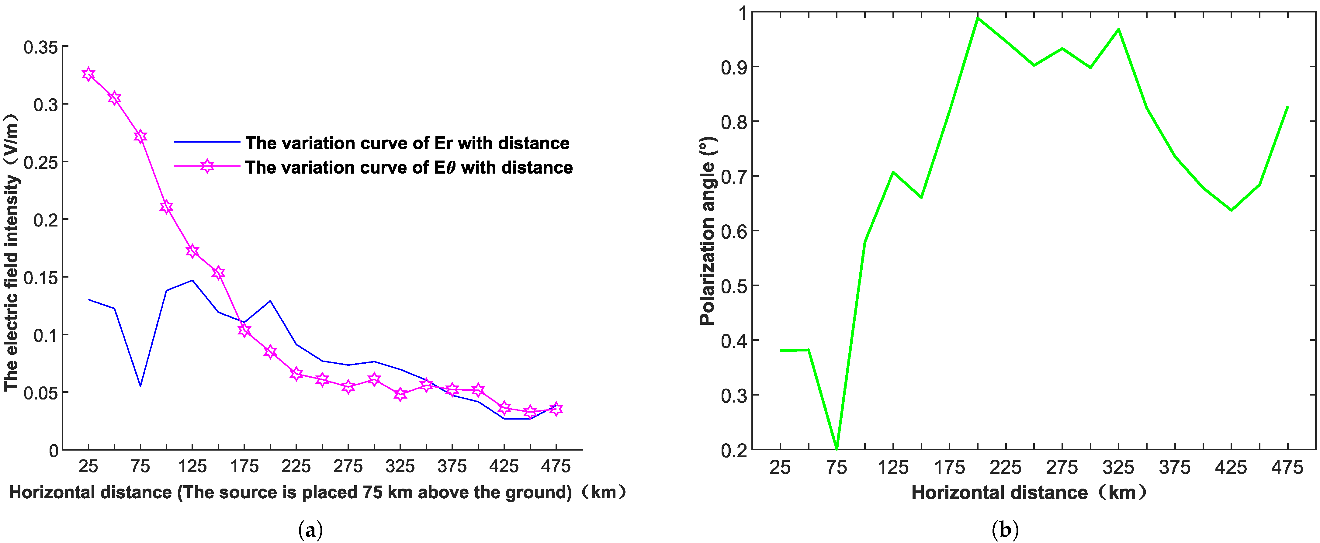
3.2.2. An Analysis of the Amplitude Attenuation, Phase-Distribution, and Polarization Characteristics of VLF Electromagnetic Waves in the Horizontal Propagation Direction of the Ionosphere

This paper provides two calculation examples to calculate the variation of the electric-field intensity with the distance when the horizontal dipole source is placed on the ground and 75 km away from the ground. The following are the resulting graphs of the two simulation examples.

Example 1: Horizontal dipole source; the source adopts a time-harmonic field and is placed on the ground. Observation points are set on the ground in sequence, and the horizontal distance from the source is 5–475 km. The curves of $E_r$ and $E_{\theta }$ varying with the distance obtained by the simulation are shown in Figure 7a.

The polarization characteristics under this kind of calculation example are analyzed, and the variation curve of the polarization angle with distance is obtained through simulation, as shown in Figure 7b.

Example 2: Horizontal dipole source. The source adopts a time-harmonic field and is placed 75 km away from the ground. Observation points are set in sequence at a height of 75 km from the ground. The horizontal distance from the source is 5–475 km. The curves of and varying with the distance are obtained through simulation, as shown in Figure 8a. The polarization characteristics under this kind of calculation example are analyzed, and the variation curve of the polarization angle with distance is obtained through simulation, as shown in Figure 8b.

During the propagation of VLF electromagnetic waves, the variation of ionospheric electron density in the horizontal direction is relatively small, so the phase is also less affected by the ionosphere. The phase will be nonlinearly changed due to the influence of the ionosphere. When the frequency is 20 kHz in the horizontal direction during the propagation process, observation points are set every 5 km within the range of 1–200 km in the horizontal direction at the corresponding heights to record the data of the electromagnetic field with respect to time. Then, the phase at each position is obtained by using the phase-lag method, so that the phase-change curve of the field quantity Er in the horizontal direction can be drawn as shown in Figure 9. In fact, when the distance is not far, the horizontal variation of the ionosphere is relatively small, which means that the phase of electromagnetic waves propagating in the horizontal direction will not be affected. The phase-change characteristics of electromagnetic waves in the horizontal direction can also serve as a reference for comparison with other situations.

It can be observed that the phase of the electromagnetic wave propagating in the horizontal direction to 200 km at the ground height remains almost always linearly changing. This indicates that when the parameters of the ionosphere in the model do not change in the horizontal direction, the propagation of the electromagnetic wave in the horizontal direction will not be nonlinearly affected by the change in the ionosphere parameters, so its phase curve remains linearly changing. In fact, when the distance is not far, the change of the ionosphere in the horizontal direction is indeed relatively small. That is to say, the phase of the electromagnetic wave propagating in the horizontal direction will not be affected. The phase-change characteristics of the electromagnetic wave in the horizontal direction can also be used as a reference for comparison with other situations.

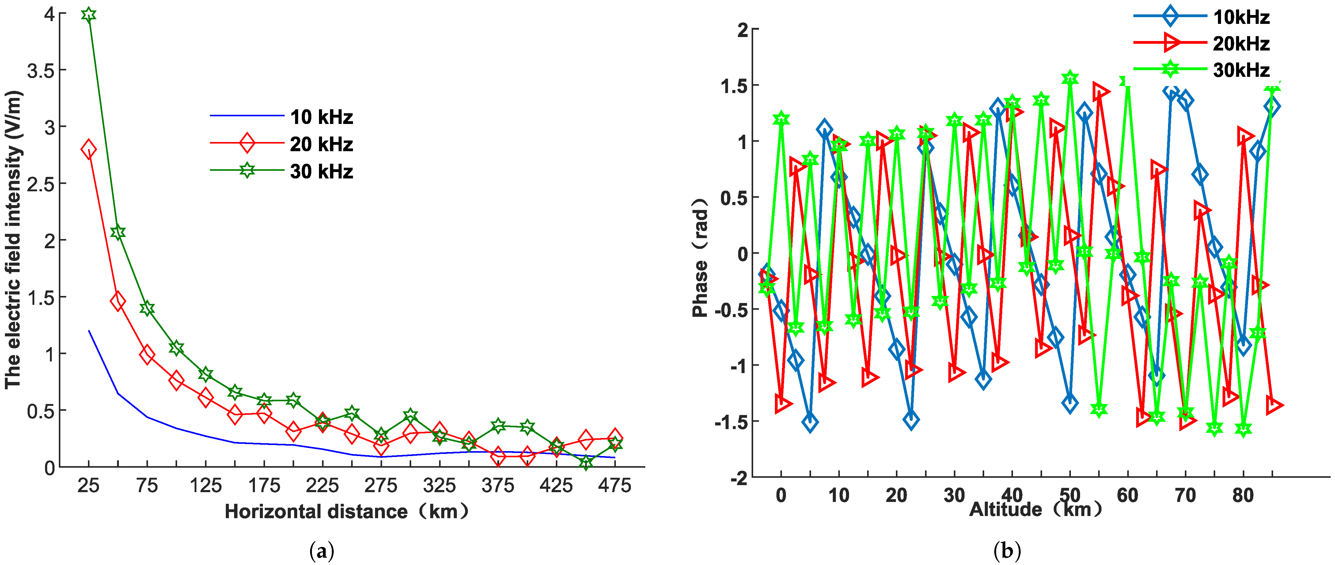
3.2.3. The Amplitude Attenuation and Phase-Distribution Characteristics of VLF Electromagnetic Waves with Different Frequencies When Propagating in the Ionosphere

VLF electromagnetic waves with frequencies of 10 kHz, 20 kHz, and 30 kHz were adopted to study the influence of sinusoidal electromagnetic waves of different frequencies on the amplitude and phase, as shown in Figure 10a,b.

Figure 10a shows the variation curves of the $E_r$ value with the horizontal distance when the horizontal dipole sources of different frequencies are placed on the ground, and Figure 10b gives the variation curves of the phase of Er of the vertical electric dipole sources of different frequencies when placed on the ground with the vertical height distance.

For VLF electromagnetic waves, when electromagnetic waves of different frequencies propagate in the horizontal direction, the higher the frequency, the greater the amplitude value. The higher the frequency, the greater the influence of the ionosphere on the phase of electromagnetic waves with lower radiation frequencies, causing phase anomalies at lower heights. The opposite is true for electromagnetic waves with relatively higher frequencies.

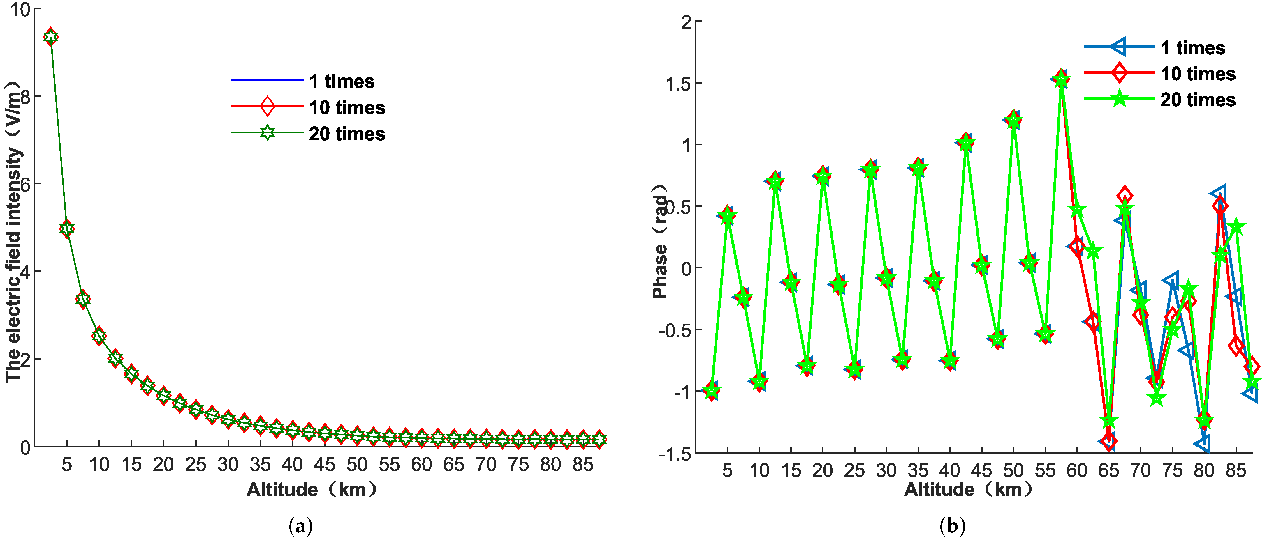
3.2.4. The Influence of Electron Density Variation on Amplitude and Phase

The electron density was amplified by 20 times and 10 times, respectively, and compared with the standard parameters to study the influence on the amplitude and phase of the electromagnetic wave when the electron density was amplified. The amplitude and phase-variation curves are shown in Figure 11a,b. Figure 11a shows the variation curves of the Er amplitude value with the vertical distance when the vertical dipole source is placed on the ground under different electron densities, and Figure 11b gives the variation curves of the phase of Er of the vertical dipole source placed on the ground under different electron densities with the vertical height distance. For the electron density, it gradually increases with the increase in height, which will cause the phase of the electromagnetic wave to be abnormal at the same time; that is to say, the greater the electron density, the greater the impact. When it reaches a certain extent, it will cause the phase of the electromagnetic wave to be inconsistent. However, the simulation found that in the low ionosphere region, with the increase in the electron density, the amplitude value of the electric-field intensity basically does not change. This may be due to the small thickness of the ionosphere used in the simulation. Currently, the IRI international reference ionosphere is being studied to verify the correctness of this phenomenon.

The change in phase is influenced by both electron density and collision frequency. At lower altitudes, the values of electron density and collision frequency are insufficient to cause a change in the phase of electromagnetic waves. When reaching around 60 km, they begin to affect the VLF electromagnetic waves.

3.2.5. The Influence of the Change in Collision Frequency on the Phase

The collision frequencies were amplified by 20 times and 10 times, respectively, and compared with the standard parameters to study the influence on the phase of the electromagnetic wave when the collision frequency was amplified and reduced. The phase-variation curve is shown in Figure 12. Figure 12 shows the variation curve of the Er phase value with the vertical distance when the vertical electric dipole source is placed on the ground under different collision frequencies.

When the collision frequency is amplified, as the amplification factor increases, the abnormal situation of the phase becomes more obvious. The phase becomes different from 60 km above the ground. When the collision frequency is amplified by 20 times, the height at which abnormalities occur increases accordingly, and abnormalities occur at 73 km.

4. Discussion

In this paper, a more accurate time-domain finite-difference algorithm model under the spherical coordinate system based on UPML boundary is established, which effectively solves the reflection problem existing in the PEC boundary. This algorithm is used to numerically calculate the field-intensity attenuation and polarization angle of VLF waves in the ionosphere, and compared and analyzed with the traditional algorithm to verify the accuracy of the algorithm.

On this basis, single-frequency signals are used to study the relationship between the phase, amplitude, and ionospheric parameters’ propagation of VLF electromagnetic waves in the magnetized plasma ionosphere. From the simulation results, it can be seen that in the vertical direction, the phase of electromagnetic waves at lower heights basically changes linearly, while the influence of the ionosphere on electromagnetic waves at a higher height causes the phase-detached linear change. The lower the frequency of electromagnetic-wave radiation, the lower the probability of phase anomalies occurring at the altitude in its propagation. The electron density and collision frequency of the ionosphere will also have different effects on the phase of electromagnetic waves when they change. When the electron density increases or the collision frequency decreases, it will lead to an increase in the phase impact of the ionosphere, causing the phase abnormality of electromagnetic waves at a lower altitude. The research results of this paper provide theoretical support for the engineering implementation of on-board very-low-frequency communication, but the actual ionospheric propagation mechanism is more complicated. VLF downlink analysis, receiver design, and ionospheric noise interference are the focus of the next study.

The research results of this article provide theoretical support for the engineering implementation of spaceborne very-low-frequency communication, but the actual ionospheric propagation mechanism is more complex. The analysis of VLF downlink, receiver design, and ionospheric noise interference are the focus of the next research step.

References

1. Yang, H.J. Latest development progress and trends of foreign data relay satellite systems. Telecommun. Eng. 2016, 56, 109–116. [Google Scholar]
2. Tamagnone, M.; Gomez-Diaz, J.S.; Mosig, J.R.; Perruisseau-Carrier, J. Reconfigurable teraherz plasmonic antenna concept using a graphene stack. Appl. Phys. Lett. 2012, 101, 836–842. [Google Scholar] [CrossRef]
3. Qu, Z.H.; Lai, M.Q. A review on electromagnetic, acoustic, and new emerging technologies for submarine communication. IEEE Access 2024, 12, 12110–12125. [Google Scholar] [CrossRef]
4. Lehtinen, N.G.; Inan, U.S. Full-wave modeling of transionospheric propagation of VLF waves. Geophys. Res. Lett. 2009, 36, 151–157. [Google Scholar] [CrossRef]
5. Su, Y.; Xu, Z.W. Numerical calculation of hierarchical transmission model of electromagnetic wave communication through formation based on FDTD. IEEE Access 2016, 35, 123–126. [Google Scholar]
6. Liu, H.C.; Liang, H. Design of an anti-interference digital receiver for satellite mobile communication systems in low SNR application. Telecommun. Eng. 2014, 54, 1418–1423. [Google Scholar]
7. Zhao, S.F.; Shen, X.H. Full wave calculation of VLF wave penetrated into satellite altitude ionosphere. IEEE Access 2015, 35, 178–184. [Google Scholar] [CrossRef]
8. Alexeff, I.; Anderson, T.; Parameswaran, S.; Pradeep, E.P.; Hulloli, J.; Hulloli, P. Experimental and theoretical results with plasma antennas. IEEE Trans. Plasma Sci. 2006, 34, 166–172. [Google Scholar] [CrossRef]
9. Bilitza, D. International reference ionosphere 200. Radio Sci. 2001, 36, 261–275. [Google Scholar] [CrossRef]
10. Yang, H.W.; Liu, Y. Numerical analysis of the reflection and absorption of electromagnetic wave in nonuniform magnetized plasma slab. Int. J. Light Electron Opt. 2012, 123, 371–375. [Google Scholar] [CrossRef]
11. Hu, X.W.; Liu, M.H. Propagation of an electromagnetic wave in a mixing of plasma-dense neutral gas. Plasma Sci. Technol. 2004, 6, 2564–2566. [Google Scholar]
12. Li, H.J.; Liu, D.C. Propagation of strong electroma-genetic pulse in space. In Proceedings of the Tenth National Antiradiation Electronics and Electromagnetic Pulse Annual Academic Conference, Sanya, China, 1 July 2009. [Google Scholar]
13. Shang, J.N.; Li, L.; Liu, C.J. Exploration and experiment of low information rate satellite communicationsystem in S-band. Telecommun. Eng. 2016, 56, 54–59. [Google Scholar]
14. Ye, Z.H.; Liao, C. Analysis of electromagnetic pulse propagation in the ionosphere. Sci. Technol. Eng. 2011, 11, 4449–4452. [Google Scholar]
15. Wu, Y.L.; Ge, D.B. Analysis of electromagnetic wave propagation in ionosphere by using FDTD combined with Z transform method. J. Hangzhou Inst. Electron. Eng. 2002, 22, 57–60. [Google Scholar]
16. Mur, G. Absorbing boundary conditions for the finite-difference approximation of the time-domain electromagnetic-field equations. IEEE Trans. Electromagn. Compat. 1981, 23, 377–382. [Google Scholar] [CrossRef]
17. Wang, J.; Zhou, B.; Shi, L.; Gao, C.; Chen, B. A Novel 3-D HIE-FDTD Method With One-Step Leapfrog Scheme. IEEE Trans. Microw. Theory Tech. 2014, 62, 1275–1283. [Google Scholar] [CrossRef]
18. Zhang, Q.; Zhou, B. A Novel HIE-FDTD Method with Large Time-Step Size [Programmer’s Notebook]. IEEE Antennas Propag. Mag. 2015, 57, 24–28. [Google Scholar] [CrossRef]
19. Dong, M.; Chen, J.; Zhang, A. Fourth-order hybrid implicit and explicit-FDTD method. Int. J. Numer. Model. Electron. Netw. Devices Fields 2006, 29, 181–191. [Google Scholar] [CrossRef]
20. Sounas, D.L.; Caloz, C. Gyrotropy and nonreciprocity of graphene for microwave applications. IEEE Trans. Microw. Theory Tech. 2008, 60, 901–904. [Google Scholar] [CrossRef]
21. Chen, Z. A finite-difference time-domain method without the Courant stability conditions. IEEE Microw. Guid. Wave Lett. 1999, 9, 441–443. [Google Scholar]
22. Moore, R.C.; Agrawal, D. ELF/VLF wave generation using simultaneous CW and modulated HF heating of the ionosphere. J. Geophys. Res. Space Phys. 2011, 116, A04217. [Google Scholar] [CrossRef]
23. Yee, K. Numerical solution of initial boundary value problems involving Maxwell’s equations in isotropic media. JIEEE Trans. Antennas Propag. 1966, 14, 302–307. [Google Scholar]
24. Cho, M.; Rycroft, M.J. Computer simulation of the electric field structure and optical emission from cloud-top to the iono-sphere. J. Atmos. Sol. Terr. Phys. 1988, 60, 871–888. [Google Scholar] [CrossRef]
Figure 1. Electromagnetic-wave propagation model in the ionosphere.
Electronics 14 01545 g001
Figure 2. Schematic diagram of VLF propagation model.
Electronics 14 01545 g002
Figure 3. A simulation model with UPML.
Electronics 14 01545 g003
Figure 4. The electric-field values calculated by the FDTD algorithm and the proposed HIE-FDTD algorithm.
Electronics 14 01545 g004
Figure 5. (a) A comparison of the daytime data of field-intensity attenuation between the algorithm proposed in this paper and the traditional algorithm; (b) a comparison of the nighttime data of field-intensity attenuation between the algorithm proposed in this paper and the traditional algorithm.
Electronics 14 01545 g005
Figure 6. (a) A comparison of the daytime data of the phase between the algorithm proposed in this paper and the traditional algorithm; (b) a comparison of the nighttime data of the phase between the algorithm proposed in this paper and the traditional algorithm.
Electronics 14 01545 g006
Figure 7. (a) The variation curves of and with distance are obtained through simulation; (b) the curve of the polarization angle varying with distance.
Electronics 14 01545 g007
Figure 8. (a) The variation curves of E r and E θ with distance; (b) the curve of polarization angle varying with distance.
Electronics 14 01545 g008
Figure 9. The phase-change curve of the horizontal dipole source in the horizontal direction at ground level.
Electronics 14 01545 g009
Figure 10. (a) The amplitude variation curves of sinusoidal electromagnetic waves of different frequencies within 1–500 km; (b) the phase-variation curves of sinusoidal electromagnetic waves of different frequencies within 1–90 km.
Electronics 14 01545 g010
Figure 11. (a) The electric-field intensity curves when the electron density is amplified compared with the standard situation; (b) the phase curves when the electron density is amplified compared with the standard situation.
Electronics 14 01545 g011
Figure 12. The phase curve when the collision frequency is amplified compared with the standard situation.
Electronics 14 01545 g012