Hyperspectral LiDAR for Subsea Exploration: System Design and Performance Evaluation

Abstract

Hyperspectral LiDAR (HSL) is a promising active detection technique for underwater positioning and remote sensing, enabling the simultaneous acquisition of three-dimensional topographic and spectral information of underwater targets. This study presents an advanced underwater hyperspectral LiDAR (UDHSL) system with a spectral range of 450–700 nm, adjustable spectral bandwidth of 10–300 nm, and tunable repetition frequency of 50 kHz to 1 MHz. The system achieves high precision with a laser divergence angle of ≤1 mrad, pulse width of 7 ns, laser energy of 7.5 µJ, ranging resolution of 1.13 cm and ranging accuracy of 1.02 m@distance of 27 m. Hyperspectral point clouds spanning 11 bands (450–650 nm) are generated during 3D pool experiments. The distance-colored point clouds precisely align with the geometric characteristics of targets, the normalized intensity-colored point clouds across spectral bands exhibit discriminative capabilities for target identification, and the color-composite point clouds approximate the true colors of targets, collectively validating the system’s ability to concurrently acquire spectral and topographic data. These results underscore the potential of this technology for underwater exploration and positioning applications.

1. Introduction

Hyperspectral LiDAR (HSL) systems hold great potential for the simultaneous acquisition of spectral and spatial information, especially in challenging underwater environments. This system combines spatial mapping capabilities (which are crucial in LiDAR-based positioning systems) with advanced spectral analysis technology to identify material composition. This integration provides the system with the advantages of both spectral and spatial information. This significantly enhances detection accuracy and reliability. Furthermore, with high-precision spatial data and accurate spectral analysis, the system facilitates precise measurement of underwater objects, further expanding the application of LiDAR technology in complex underwater environments and advancing underwater detection technology to new frontiers. However, these systems have not yet been deployed in the underwater domain.

In recent years, hyperspectral LiDAR has achieved significant progress in atmospheric and terrestrial observations. In 2011, Woodhouse et al. [1] proposed a four-wavelength (531, 550, 660, and 780 nm) multispectral LiDAR based on an Nd: YAG-pumped laser and a commercial tunable laser system, enabling the measurement of the normalized difference vegetation index (NDVI) and photochemical reflectance index (PRI). In 2014, Wallace et al. [2] employed a supercontinuum light source and an acousto-optic tunable filter (AOTF) covering the 500–850 nm range with eight selectable wavelengths, facilitating further exploration of forest structures and physiological parameters. In 2010, the Finnish Geospatial Research Institute (FGI) developed a dual-channel LiDAR (600–2000 nm), and in 2012, it constructed a 450–1050 nm full-waveform system based on a supercontinuum light source capable of acquiring 16 wavelength channels, which were used to measure the backscattering reflectance and NDVI of Norway spruce [3,4]. The FGI is dedicated to research on hyperspectral LiDAR technology and has been deeply engaged in relevant studies applying hyperspectral LiDAR technology to forestry remote sensing, forestry resource exploration, and other fields [5,6,7]. In 2013, Wuhan University combined a supercontinuum light source, a grating-based dispersion system, and an APD array to build a hyperspectral LiDAR providing 32 channels with a spectral resolution of 12 nm, covering 450–910 nm [8,9,10]. In the same year, the Aerospace Information Research Institute (formerly the Institute of Remote Sensing and Digital Earth) of the Chinese Academy of Sciences developed a four-wavelength full-waveform multispectral LiDAR prototype, later expanded in 2016 to 32 channels (409–914 nm) with an average spectral resolution of 17 nm [11,12,13,14]. Meanwhile, Wang et al. [15] at the Aerospace Information Research Institute (formerly the Institute of Optoelectronics) utilized grating-based spectral dispersion to create an eight-channel full-waveform LiDAR spanning the visible–near-infrared–shortwave-infrared range, which was subsequently extended to 17 channels (450–1600 nm). Li Wei et al. [16] employed a supercontinuum laser and an AOTF covering 500–1000 nm with a 10 nm spectral resolution, obtaining 51-channel data for plant leaf measurements.

These studies underscore that current hyperspectral LiDAR prototypes primarily target atmospheric and terrestrial applications, yielding substantial advancements in vegetation monitoring, forestry, and mineral classification. Nevertheless, no mature hyperspectral LiDAR system has been deployed for underwater detection.

Unlike air, seawater has unique challenges that significantly impact the performance of LiDAR systems [17,18,19,20]. Current underwater detection systems confront three core technical limitations: (1) inadequate environmental adaptability: poor mechanical stability, low spectral matching accuracy, and lack of integrated waterproofing/thermal management designs compromise long-term underwater reliability; (2) pronounced aquatic attenuation effects: dual absorption-scattering interactions during optical transmission cause nonlinear accumulation of ranging errors with distance; and (3) unstable radiation characteristics: coupled laser pulse energy fluctuations and complex scattering effects significantly degrade spectral inversion confidence. These technical barriers highlight the urgent need for developing specialized high-reliability underwater detection hyperspectral LiDAR (UDHSL) systems.

To address these challenges, we have developed an UDHSL system that integrates a supercontinuum laser source with a tunable filter. This combination enables precise wavelength selection while ensuring the mechanical stability of the system, thereby enhancing data accuracy and overall quality. The UDHSL system offers a comprehensive approach to underwater exploration by simultaneously capturing spectral characteristics and spatial terrain data. By using a tunable filter and a supercontinuum laser, the system can efficiently collect wavelengths most suitable for varying deep-sea conditions, thereby mitigating wavelength-selective water attenuation effects and enhancing overall data reliability.

This study has achieved the engineering application of the UDHSL for the first time. It details the architecture of the UDHSL system, which includes four modules: laser emission, receiving optics, detection, and scanning modules. The system achieves a spectral range of 450–700 nm, an adjustable spectral bandwidth of 10–300 nm, and a tunable repetition frequency of 50 kHz–1 MHz, ensuring high flexibility and performance. Experimental results from underwater tests validate the effectiveness of the system. To evaluate system performance of ranging accuracy, Echo signals were collected at 12 discrete distances ranging from 2.88 m to 27.03 m, and the ranging accuracy was measured as 1.02 m@distance of 27 m. Three-dimensional pool experiments generated hyperspectral point clouds across 11 bands (450–650 nm), with corrected colors that were approximately the true colors of targets. These results demonstrate the UDHSL system’s ability to simultaneously achieve high-precision distance measurement and spectral discrimination of multiple targets underwater. It is a significant asset for detailed and reliable underwater surveys in subsea exploration and target detection.

2. System Design

Deep-sea exploration scenarios impose strict requirements on acquiring three-dimensional terrain information while also emphasizing the importance of capturing the spectral characteristics of surrounding substances. Based on a thorough analysis of the current development status of hyperspectral LiDAR technology, this study integrates a supercontinuum laser with a tunable filter to construct a hyperspectral LiDAR system that meets these demands successfully.

The schematic of the proposed UDHSL system is shown in Figure 1. The UDHSL system mainly includes a laser emission module, a receiving optics module, a detection module, a scanning module, and a control module. All these modules are installed in a self-designed waterproof shell, enabling water-cooling functionality with an optical window for laser transmission.

The laser emission module primarily consists of a supercontinuum laser, a tunable filter, and an emission optical system. The supercontinuum laser serves as the light source for the emission module. The tunable filter selects specific wavelengths from the supercontinuum laser. The emission optical system directs the filtered laser pulses toward a target. The module is designed to emit laser signals at distinct time intervals, with each interval corresponding to a different wavelength.

The receiving optical system collects the laser echo signals of multiple wavelengths. These collected signals are focused on the photodetector. The photodetector converts the collected optical signals into electrical signals.

The detection module processes the electrical signals. An amplification circuit in the detection module amplifies these electrical signals. After amplification, the signals undergo analog-to-digital conversion in the data acquisition system. The data acquisition system is used to collect and store the converted digital information.

The scanning module is used to synchronize the emission beam direction with the receiving system’s instantaneous field of view. The scanning module also controls the movement of both the emission and receiving systems.

The main indicators of the system are show in

Table 1. Main indicators of UDHSL system.

Spectral band range	450 nm~700 nm
Spectral bandwidth	10 nm~300 nm adjustable
Repetition frequency	50 kHz~1 MHz adjustable
Laser divergence angle	≤1 mrad
Pulse width (FWHM)	7 ns
Laser energy (@450 nm~700 nm)	7.5 μJ
Aperture of optical system	202 mm
Scanning field of view	Azimuth: ±35° Pitch: −5° to 20°
Operating depth	≤10 m
Ranging resolution	1.13 cm
Ranging accuracy	1.02 m@distance of 27 m

.

2.1. Supercontinuum Laser Source

To ensure the detection range of the hyperspectral LiDAR system, a supercontinuum laser with relatively high single-pulse energy is selected. The laser is compact, lightweight, and optimized with air cooling to meet system integration requirements. It consists of a high-energy pump laser and photonic crystal fiber. The pulse repetition rate of the laser ranges from 50 kHz to 1 MHz. The pulse width is 7 ns. The spectral coverage ranges from 400 nm to 2400 nm. The maximum single-pulse energy is 100 μJ. The single-pulse energy in the 400 nm to 720 nm range is 21 μJ. After filtering, the single-band single-pulse energy is 1.1 μJ (with a bandwidth of ≥20 nm @450 nm~700 nm). The beam quality factor, M², is 1.25. Figure 2 shows the typical supercontinuum output spectrum of the laser we use here.

2.2. Tunable Filter and Beam Shaping

To achieve the spectral gating specified for the hyperspectral LiDAR system, a combination of a tunable filter and a supercontinuum light source is used. The tunable filter is a plug-and-play spectral module. It uses a linear variable filter (LVF) that provides high transmission efficiency. The filter system consists of a filtering device, a driver module, and control software. Users can set the wavelength range between 400 nm and 740 nm through the control software. The output wavelength bandwidth is adjustable between 10 nm and 300 nm, with a typical value greater than 20 nm. The entire filter system provides spatial collimated light output with a transmittance of 71%.

Two linear variable filters are used in the system. The wavelength linear variation rate of the filter is approximately 9 nm/mm. In order to achieve an output spectrum bandwidth of less than 20 nm, the spot size must be smaller than 2 mm. The collimation lens of the laser adjusts the spot size. A smaller spot size can lead to excessive energy density, which may damage the filter. In order to prevent damage, a short-pass filter with a cutoff wavelength of 750 nm is added in front of the main filter. The short-pass filter is used to block near-infrared light. It is installed at an angle of 1–2° to prevent reflected light from returning to the laser and causing damage.

The filtered light has a large divergence angle that does meet the final application requirements. Therefore, a beam expansion system is integrated into the setup to adjust this divergence. The entire beam expansion system is fixed to the filter housing using a cage structure to ensure stability during operation.

2.3. Selection of Work Spectrum Segments

The selection of the working spectral band is based on the spectral transmission window of clean seawater. The main transmission window of clean seawater occurs at 480 nm. According to the spectral attenuation distribution of water in the wavelength range from 200 nm to 800 nm [21], considering both the attenuating effect of water and the energy distribution of the light source, the range from 400 nm to 720 nm is selected as the working spectral band of the system. By choosing blue-green light with high transmittance and high energy from the laser light source, long-range distance measurement can be achieved to support three-dimensional seabed topographic surveying. At relatively short distances, spectral data across the entire visible spectrum range can be collected for underwater exploration.

2.4. Transceiver Optical System

Based on the requirements of deep-sea exploration, the receiving optical system must be compact and capable of covering a working distance of 3 to 12 m without needing to adjust the focal plane. Therefore, the optical system design must be compact and have a sufficiently large detector photosensitive area. In this study, a PMT photodetector with an 8 mm photosensitive area was selected (Hamamatsu H10721 [22]), and a matching optical system was designed. Figure 3 shows the design scheme, which includes a parabolic mirror with a diameter of 210 mm and a central obscuration diameter of 50 mm, resulting in an effective aperture of approximately 202 mm. Figure 4 shows that at working distances of 3 m, 7.5 m, and 12 m. The design results indicate that the spot diameter at the focal plane is a maximum of approximately 6 mm at both 3 m and 12 m. The mirror is made of low-density fused silica glass, with a silver coating and a protective layer to improve reflectivity to over 85%.

2.5. Scanning Mechanism

The scanning mechanism is implemented using a two-dimensional turntable. This turntable is a gimbal platform that rotates around two axes. The system is composed of an elevation axis and an azimuth axis. This mechanism is used for precise target pointing and tracking targets for the detector head. The two-dimensional turntable includes a base, an azimuth main support structure, and an elevation main support structure. It also features a detector-mounting bracket, an elevation axis, and an azimuth axis. The drive mechanism components and electronic control module are also part of the assembly. The drive mechanism includes an elevation motor reducer and elevation axis, as well as an azimuth motor reducer and azimuth axis. The axis feedback element is a single-turn encoder. The encoder type is a 16-bit absolute encoder with a resolution of no greater than 0.0055°. The pointing accuracy of the rotation is better than 0.1°.

2.6. System Integration

The system mainly consists of an optical–mechanical scanning system and control cabinet, as shown in Figure 5. The system utilizes a fiber-optic connection between the laser and the filter optical machine head. Although this approach introduces some energy loss, it effectively lowers the mechanical center of gravity and achieves a more compact and rational layout, thus improving the system’s pointing stability during operation. The system, equipped with a 10 GHz sampling data acquisition card, attains a ranging resolution of 1.13 cm underwater.

For underwater experiments, the system is enclosed within a dedicated waterproof casing equipped with composite waterproof interfaces and a specially designed optical window, as shown in Figure 6. The optical window is made of H-K9L optical glass with a diameter of 450 mm, and anti-reflection coatings (air-to-glass and glass-to-water coatings) are applied on both surfaces, significantly increasing the transmittance from approximately 80% to 99.5%. The anti-reflection coating significantly reduces laser energy loss, preventing noise and detector saturation caused by close-range reflections.

3. Experimental Data Collection and Analysis

3.1. Pipe Experimental Environment

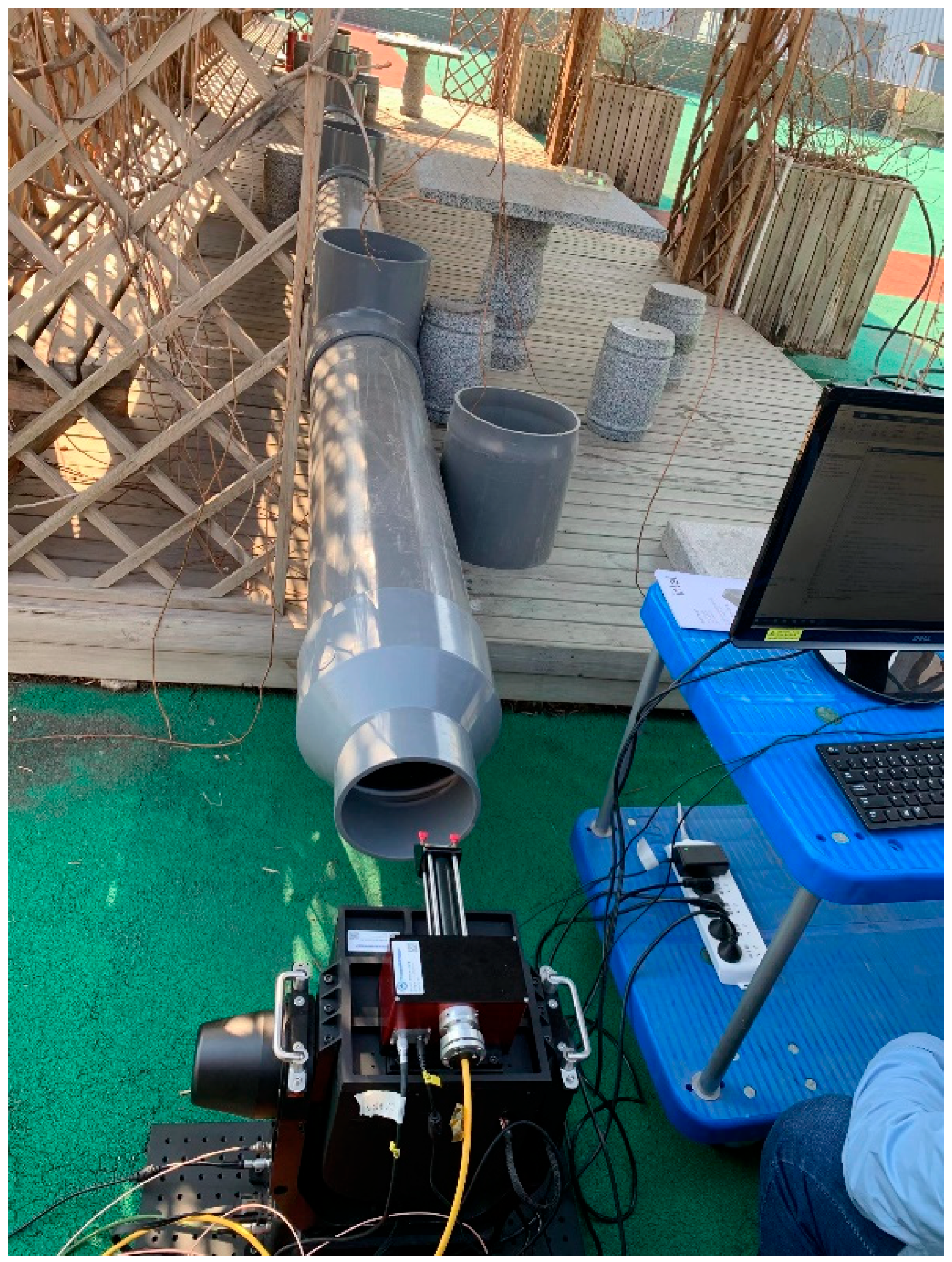
In order to study the characteristics of hyperspectral LiDAR in deep-sea exploration, a testing platform was built using a water pipe, as shown in Figure 7. The water pipe was made of opaque PVC material, and one end was a coated optical glass window with the same parameters as the glass window of the waterproof shell. The water pipe consisted of approximately 2 m long straight pipes and three-way components connected at intervals. At the three-way opening, targets can be placed, and a cover was provided to ensure a dark environment inside the water pipe. Before the experiment, we rinsed the water pipe with clean water and then added fresh tap water. We allowed it to stand for at least 2 h before experimenting.

The test target was a waterproof standard reflectivity target, as shown in Figure 8. It was placed at a specific distance for data collection.

3.2. Adjustment and Parameter Settings

During the experiment, the UDHSL system was placed outside the light window, the laser was emitted into the water in the pipe, and the echo was collected. At the same time, shading treatment was applied to the environment where the UDHSL system was located. The system parameter settings were as follows: spectral range: 450 nm–610 nm; spectral width: 10 nm, with 17 bands; repetition frequency: 50 kHz, repeat measurements of 20 pulses per frequency band; and 10 GHz sampling. Using the AC-S water absorption and attenuation meter from WET Labs, Philomath, OR, USA, measurements of fresh tap water in a water pipe showed an attenuation coefficient of approximately 0.05 m⁻¹ at a wavelength of 550 nm.

3.3. Collection of Test Data

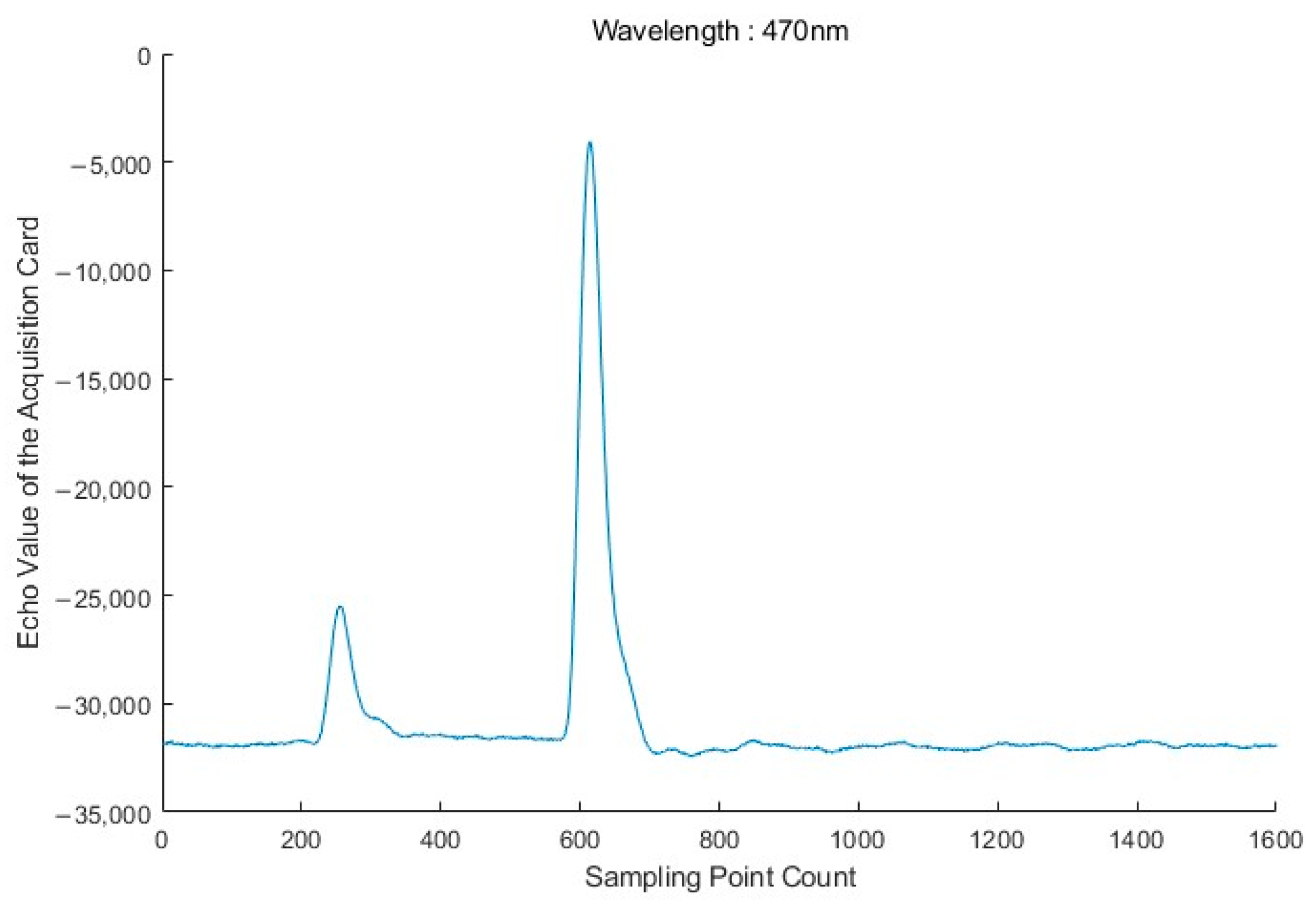
The echo data of the full waveform LiDAR are shown in Figure 9 (displayed at a wavelength of 470 nm).

In the figure, the abscissa is the sampling point count k of the full waveform digital acquisition card (ADC), and the ordinate represents the Echo_Value (a dimensionless quantity) of the acquisition card, which is essentially the intensity (W/m²). The specific conversion relationship of value and intensity is as follows:

$$\mathrm{V}\mathrm{a}\mathrm{l}\mathrm{u}\mathrm{e}=\mathrm{I}\mathrm{n}\mathrm{t}\mathrm{e}\mathrm{n}\mathrm{s}\mathrm{i}\mathrm{t}\mathrm{y}\ast S_d\ast S_k\ast {\displaystyle \frac{G_{amp}}{V_{FS}}}\ast 2^N-bias,$$

(1)

where

$S_d$: the effective area of the detector, m².

$S_k$: the cathode radiant sensitivity of the detector, A/W.

$G_{amp}$: the amplifier gain, V/A.

$V_{FS}$: the full-scale input voltage range of the ADC, V.

N: the number of bits for the full-scale range.

$bias$: the bias value.

For a given system, the parameter ${k_s=S}_d\ast S_k\ast {\displaystyle \frac{G_{amp}}{V_{FS}}}\ast 2^N$ is a constant. Thus, we have

$$\mathrm{V}\mathrm{a}\mathrm{l}\mathrm{u}\mathrm{e}\_\mathrm{c}\mathrm{o}\mathrm{r}\mathrm{r}\mathrm{e}\mathrm{c}\mathrm{t}=\mathrm{V}\mathrm{a}\mathrm{l}\mathrm{u}\mathrm{e}+bias=k_s·\mathrm{I}\mathrm{n}\mathrm{t}\mathrm{e}\mathrm{n}\mathrm{s}\mathrm{i}\mathrm{t}\mathrm{y},$$

(2)

The sampling frequency is $f=10 \mathrm{GHz}$, and the distance is calculated through the LiDAR distance formula.

$$\mathrm{L}={\displaystyle \frac{c}{2n_{\lambda }}}·{\displaystyle \frac{k}{f}},$$

(3)

where

$\mathrm{L}$: distance, m.

$c$: speed of light, ${3\times 10}^8 \mathrm{m}/\mathrm{s}$.

$n_{\lambda }$: the refractive index at a wavelength of $\lambda$.

$k$: the sampling point count of the full waveform digital acquisition card.

$f$: the sampling frequency, Hz.

Specifically, when $k=1$ and $n_{\lambda }=n_{water}=1.33$ (the approximate refractive index of water), the calculated ranging resolution is $\Delta \mathrm{L}=1.13 \mathrm{cm}$, which represents the theoretical limit of the system’s distance measurement capability.

The first echo detected by the system is the reflection echo from the window glass, and the second echo is the reflected echo from the target. Figure 10 shows the echo waveform data of 17 bands of a single diffuse reflector plate.

3.4. Normalization of Test Data

In the process of laser detection, the first echo is regarded as the reference pulse, which carries the energy emitted by the laser. Due to the inherent instability of single-pulse energy, this instability can have a significant impact on data applications. This is because the echo energy actually contains the spectral information of the target, and the fluctuations of energy will interfere with the accurate interpretation of the true spectral characteristics of the target. In order to ensure the reliability and validity of the data, it is particularly important to eliminate the interference from emission intensity on the echo values. Therefore, we use the energy data of the reference pulse to normalize the energy data of other echoes. In this way, the influence of emission intensity on the echo values is effectively eliminated, thus greatly improving the consistency of the data and laying a solid foundation for subsequent data applications and analyses. The normalization process is as follows:

(a) Bias Correction: to correct systemic offsets, a bias value of $2^{15}$ from the full-waveform digital acquisition card was added to both Echo_Value and Transmit_ Value (reference pulse):

$$\mathrm{E}\mathrm{c}\mathrm{h}\mathrm{o}\_\mathrm{V}\mathrm{a}\mathrm{l}\mathrm{u}\mathrm{e}\_\mathrm{C}\mathrm{o}\mathrm{r}\mathrm{r}\mathrm{e}\mathrm{c}\mathrm{t}\mathrm{e}\mathrm{d}=\mathrm{E}\mathrm{c}\mathrm{h}\mathrm{o}\_\mathrm{V}\mathrm{a}\mathrm{l}\mathrm{u}\mathrm{e}+\mathrm{b}\mathrm{i}\mathrm{a}\mathrm{s},$$

(4)

$$\mathrm{T}\mathrm{r}\mathrm{a}\mathrm{n}\mathrm{s}\mathrm{m}\mathrm{i}\mathrm{t}\_\mathrm{V}\mathrm{a}\mathrm{l}\mathrm{u}\mathrm{e}\_\mathrm{C}\mathrm{o}\mathrm{r}\mathrm{r}\mathrm{e}\mathrm{c}\mathrm{t}\mathrm{e}\mathrm{d}=\mathrm{T}\mathrm{r}\mathrm{a}\mathrm{n}\mathrm{s}\mathrm{m}\mathrm{i}\mathrm{t}\_\mathrm{V}\mathrm{a}\mathrm{l}\mathrm{u}\mathrm{e}+\mathrm{b}\mathrm{i}\mathrm{a}\mathrm{s},$$

(5)

(b) Normalization: the corrected echo values were normalized by dividing by the corrected transmit value:

$$\mathrm{E}\mathrm{c}\mathrm{h}\mathrm{o}\_\mathrm{V}\mathrm{a}\mathrm{l}\mathrm{u}\mathrm{e}\_\mathrm{N}\mathrm{o}\mathrm{r}\mathrm{m}\mathrm{a}\mathrm{l}\mathrm{i}\mathrm{z}\mathrm{e}\mathrm{d}={\displaystyle \frac{\mathrm{E}\mathrm{c}\mathrm{h}\mathrm{o}\_\mathrm{V}\mathrm{a}\mathrm{l}\mathrm{u}\mathrm{e}\_\mathrm{C}\mathrm{o}\mathrm{r}\mathrm{r}\mathrm{e}\mathrm{c}\mathrm{t}\mathrm{e}\mathrm{d}}{\mathrm{T}\mathrm{r}\mathrm{a}\mathrm{n}\mathrm{s}\mathrm{m}\mathrm{i}\mathrm{t}\_\mathrm{V}\mathrm{a}\mathrm{l}\mathrm{u}\mathrm{e}\_\mathrm{C}\mathrm{o}\mathrm{r}\mathrm{r}\mathrm{e}\mathrm{c}\mathrm{t}\mathrm{e}\mathrm{d}}}$$

(6)

3.5. Analysis and Discussion of Intensity Stability

In order to quantify data stability, the following statistical metrics were computed for both the raw and normalized datasets:

(a) Standard Deviation (SD): this measures the dispersion of data points around the mean.

$$\mathrm{S}\mathrm{D}=\sqrt{{\displaystyle \frac{1}{N-1}}{\sum }_{i=1}^N {\left(x_i-\mu \right)}^2},$$

(7)

Here, $x_i$ represents individual measurements, and $\mu$ is the mean of the dataset.

(b) Coefficient of Variation (CV): this represents the ratio of the standard deviation to the mean, expressed as a percentage.

$$\mathrm{C}\mathrm{V}=\left({\displaystyle \frac{\mathrm{S}\mathrm{D}}{\mu }}\right)\times 100\%,$$

(8)

Computing the stability indicators yielded the following results, as shown in

Table 2. Stability.

Metric	Raw Data of Intensity	Normalized Data of Intensity
Standard Deviation (SD)	17,193.05	2.04
Coefficient of Variation (CV) (%)	298.88%	37.53%

and Figure 11.

Due to the poor stability of the laser intensity output (Echo_Value_Corrected) from the transmitting laser, the standard deviation (SD) calculated using Equation (7) was 17,193.05, and the coefficient of variation (CV) derived from Equation (8) reached 298.88%. This study followed conventional data analysis protocols and applied Equation (6) for data normalization. The calculated Echo_Value_Normalized results showed that the SD decreased to 2.04, and the CV dropped to 37.53%. These changes indicate that normalization effectively reduced the dispersion and relative variability of the dataset, aligning with typical improvement trends observed after data standardization. Further analysis revealed that the concentration of the standardized data distribution increased by approximately three orders of magnitude compared to the raw data, with the CV value reduced by 87.43%. These outcomes fall within the expected range of improvements when addressing heteroscedastic data using normalization methods. The quantitative results demonstrate that applying domain-standard data preprocessing methods significantly enhances the measurement consistency of UDHSL echo signals, thereby establishing a more reliable data foundation for subsequent analyses.

3.6. Analysis and Discussion of Echo Intensity

The following figure shows a box plot of the distribution of normalized echo intensities for five targets across different wavebands. The targets are waterproof standard reflectivity objects, as illustrated in Figure 12. In the boxplots, the graphic consists of a box and upper/lower whiskers. The box boundaries correspond to the upper quartile (Q3, third quartile) and lower quartile (Q1, first quartile) of the dataset, with a horizontal line inside the box marking the median value. The whiskers extend from the box edges to the most extreme data points within 1.5 times the interquartile range (IQR = Q3 − Q1). Outliers, represented by red plus symbols, are defined as those observations that fall outside the whisker range and demonstrate significant deviations from the main distribution of the dataset.

The figure shows that the normalized echo intensity varies across different bands for the same target, while the box plot distribution trends are similar for different targets. It suggests that the environmental factors predominantly govern the overall response mechanism. Specifically, the dramatic intensity decline at longer wavelengths aligns closely with water absorption spectra, directly confirming the dominant limitation of strong water molecular attenuation on long-wave laser energy. The observed intensity discrepancies arise from coupled physical mechanisms along transmission paths: hardware-related factors including wavelength-dependent transmittance of window materials and detector response characteristics; environmental influences primarily stemming from spectral absorption properties of water constituents (phytoplankton, CDOM, and suspended particles), and wavelength-specific attenuation.

Though normalization enhances data stability, residual dispersion persists in boxplots, which could exacerbate under complex underwater conditions (e.g., turbulence or varying suspended particle concentrations). To address these challenges, hardware improvements should focus on enhancing laser energy stability and optimizing transmittance uniformity of optical windows to reduce systematic errors. Methodological enhancements recommend implementing redundant measurements with echo intensity averaging algorithms to mitigate random noise, complemented by real-time attenuation compensation using spectral water databases to improve detection reliability.

3.7. Analysis and Discussion of Ranging Accuracy

Ranging accuracy refers to the consistency between the distance values measured by the UDHSL system and the true distances, defined as the absolute deviation between the measured mean and the true distance. To evaluate system performance, a standard diffuse reflector with 90% reflectivity was employed as the target. Echo signals were collected at 12 discrete distances ranging from 2.88 m to 27.03 m. The true distance was calibrated using a high-precision measuring tape (resolution: ±1 mm). Measurement error was calculated as the difference between the mean of repeated measurements and the true distance, while standard deviation was used to quantify the dispersion of single measurements. As shown in

Table 3. Ranging accuracy experimental data.

True Distance (m)	Measured Mean (m)	Measurement Error (m)	Standard Deviation (m)
2.88	3.04	0.16	0.25
5.20	5.49	0.29	0.21
7.54	7.90	0.36	0.15
9.79	11.02	1.23	0.59
11.56	12.23	0.67	0.30
13.73	15.01	1.28	0.45
15.97	17.26	1.29	0.38
18.17	19.47	1.30	0.26
20.36	21.56	1.20	0.28
22.60	23.58	0.98	0.18
24.85	25.83	0.98	0.07
27.03	28.05	1.02	0.06

, the experimental data analysis reveals the following:

(1) Within 20.36 m, the measurement error shows a positive correlation with target distance, i.e., the error increases nonlinearly with distance, consistent with the theoretical expectation of LiDAR ranging error behavior [23].

(2) Beyond 20.36 m, both measurement error and standard deviation decrease significantly. Spectral analysis of raw data indicates that effective echo signals at distances exceeding 20.36 m are concentrated in the 480–560 nm wavelength range (green light band). The lower attenuation coefficient of this band in water (0.3 m⁻¹ @550 nm, as measured in Section 3.2) enhances signal stability, thereby reducing error dispersion.

Key conclusions from this experiment include the following: (1) Multi-wavelength ranging introduces unnecessary interference, which degrades ranging accuracy. It is recommended to adopt a single low-attenuation wavelength (e.g., 550 nm) to improve the stability of system ranging performance. (2) Model-based correction: future research should focus on establishing an underwater laser transmission attenuation model to compensate raw ranging values, thereby further enhancing system ranging accuracy.

4. Acquisition of Underwater Hyperspectral Laser Point Clouds

4.1. Pool Experimental Environment

A light-shielding pool was selected as the site for conducting simulated marine environment tests. The pool was 50 m long, 15 m wide, and 10 m deep. A light-shielding device covered the water surface and simulated the dark optical environment of a seabed. The site was equipped with two sets of gantry frames and telescopic rods, which were, respectively, used to fix the test equipment and the target, as shown in Figure 13.

We integrated the equipment into a waterproof housing and installed it on the telescopic rod. Through the movement of the gantry frame and the telescopic rod, we fixed the equipment underwater to conduct the three-dimensional point cloud acquisition test of the underwater scene, as shown in Figure 14. The emission optical path of the UDHSL was parallel to the horizontal plane.

We arranged a three-dimensional scene at about 3 m distance. We fixed the typical ore target and the 60% standard reflectivity target on the brackets with a distance difference of 0.5 m in a staggered manner. The front side of the brackets was treated to make it black to avoid generating strong reflected light, as shown in Figure 15.

4.2. Adjustment and Parameter Settings

During the experiment, the UDHSL system was placed 3 m far from the targets. The system parameter settings were as follows: spectral range: 450 nm–650 nm; spectral width: 20 nm, with 11 bands; repetition frequency: 50 kHz, repeat measurements of 20 pulses per frequency band; and 10 GHz sampling. Using the AC-S water absorption and attenuation meter from Wetlabs, USA, measurements of the water in the pool showed an attenuation coefficient of approximately 0.3 m⁻¹ at a wavelength of 550 nm.

4.3. Scanning and Point Cloud Calculation

To scan the target scene, the two-dimensional turntable of the UDHSL rotated in both the azimuth and elevation directions. The laser beam conducted the all-round scanning of the target, thereby obtaining the multi-dimensional information of the target scene. The scanning mode was in a “zigzag” shape, as shown by the arrow directions in Figure 16.

When the LiDAR system is in operation, the digital acquisition card records the azimuth and elevation angles of the two-dimensional turntable in real time and uses them for subsequent point cloud calculations. This angle information can help the system determine the position and angle of the laser beam irradiation and then generate the corresponding point cloud data. The azimuth angle, α, is the angle between the projection of the laser beam and the y-axis, with clockwise rotation being positive; the elevation angle, β, is the angle between the laser beam and its projection. The projection of the laser beam is the projection on the plane determined by the x- and z-axes.

After calculating the distance, R, between the LiDAR and the target to be measured by combining the elevation angle and azimuth angle of the turntable at the moment of laser emission, the three-dimensional coordinate values of the laser point cloud in the Cartesian coordinate system can be calculated. The three-dimensional point cloud calculation can be completed according to the calculation results.

Taking the emission center of the UDHSL system as the origin and denoting it as $(X_0,Y_0,Z_0)$ and the coordinates of any scanning point as $(X,Y,Z)$, the calculation of the spatial coordinates of the scanning point in the Cartesian coordinate system is as follows:

$$\left\{\begin{array}{l}X=X_0+\mathrm{R}\ast \cos \beta \ast \sin \alpha \\ Y=Y_0+R\ast \cos \beta \ast \cos \alpha \\ Z=Z_0+R\ast \sin \beta \end{array}\right.,$$

(9)

After calculating the three-dimensional coordinates through the sum of distances, a point cloud with spatial coordinates can be generated where each point simultaneously contains its corresponding backscattering intensity. Shown below is the point cloud obtained from UDHSL backscattering measurements in the 550 nm wavelength range.

4.4. Analysis and Discussion of Distances

Figure 17a presents a front view (X-Z plane) of the target point cloud, color-coded by Y-coordinate values. The point cloud effectively captures the three-dimensional geometry and structural features of the targets. Notably, the nearly complete outer framework and the sponge attached to it (indicated by blue points) are clearly visible, consistent with the observations in Figure 17b. The lower Y-values of these points suggest their proximity to the origin of the device coordinate system. Furthermore, the layered arrangement of internal targets is evident, such as the quartzite (upper layer) and manganese ore (lower layer), both exhibiting echoes with low Y-values (blue points). The point cloud data exhibit comprehensive coverage of the target area with high density (no significant voids or sparse regions), indicating that the UDHSL system maintains stable data acquisition capability in underwater environments.

Figure 17c displays the top view (X-Y plane) of the target point cloud, color-coded by Y-coordinate values. Stratification along the Y-axis is observed in specific regions, primarily attributed to the ranging resolution limitations of the UDHSL. To enhance data quality, post-processing techniques such as full-waveform data resampling and high-precision waveform fitting can be implemented, thereby improving the effective ranging resolution at the algorithmic level.

4.5. Analysis and Discussion of Intensity

The experiment acquired LiDAR point clouds at multiple wavelengths. The echo intensity was normalized using a 60% standard reflectance panel, calculated by the following formula [16]:

$$I_{\mathrm{N}\mathrm{o}\mathrm{r}\mathrm{m}\mathrm{a}\mathrm{l}\mathrm{i}\mathrm{z}\mathrm{e}\mathrm{d}}(\lambda )={\displaystyle \frac{V_{\mathrm{T}\mathrm{a}\mathrm{r}\mathrm{g}\mathrm{e}\mathrm{t}}(\lambda )}{V_{\mathrm{R}\mathrm{e}\mathrm{f}\mathrm{r}\mathrm{e}\mathrm{n}\mathrm{c}\mathrm{e}}(\lambda )}}{\rho }_{\mathrm{R}\mathrm{e}\mathrm{f}\mathrm{r}\mathrm{e}\mathrm{n}\mathrm{c}\mathrm{e}}(\lambda )$$

(10)

where

$\lambda$: the wavelength (nm);

$I_{\mathrm{N}\mathrm{o}\mathrm{r}\mathrm{m}\mathrm{a}\mathrm{l}\mathrm{i}\mathrm{z}\mathrm{e}\mathrm{d}}(\lambda )$: the normalized intensity;

$V_{\mathrm{T}\mathrm{a}\mathrm{r}\mathrm{g}\mathrm{e}\mathrm{t}}(\lambda )$: the intensity value of the target;

$V_{\mathrm{R}\mathrm{e}\mathrm{f}\mathrm{r}\mathrm{e}\mathrm{n}\mathrm{c}\mathrm{e}}(\lambda )$: the intensity value of the standard reflectance target;

${\rho }_{\mathrm{R}\mathrm{e}\mathrm{f}\mathrm{r}\mathrm{e}\mathrm{n}\mathrm{c}\mathrm{e}}(\lambda )$: is the reflectance of the standard target.

The 3D UDHSL point clouds (X-Z plane) across wavelengths (450–650 nm), color- coded with normalized echo intensity, are shown in Figure 18. Key analytical results include the following: (1) Target Contour Identification: the echo intensity distribution effectively reveals the geometric contours of different targets (e.g., standard reflectance panel, sponge, quartzite), demonstrating the capability of intensity data to characterize the spatial morphology of underwater objects. (2) Spectral Signature Variations: Manganese ore exhibits significantly enhanced echo intensity in the 590–630 nm band (Figure 18h–j), while showing negligible signals (similar to the black background) in the 450–470 nm range (Figure 18a,b). Quartzite displays normalized intensity below the 60% standard target at 470 nm (Figure 18b), but exceeds the 60% standard target in the 610–630 nm band (Figure 18i,j), indicating its silicate crystalline structure preferentially reflects longer wavelengths.

To leverage these spectral–spatial features, hyperspectral feature-matching algorithms (e.g., Support Vector Machine or Random Forest classifiers) can be applied for automated target classification by training wavelength-intensity response models. Furthermore, integrating 3D point cloud intensity and geometric attributes could enhance recognition accuracy for overlapping targets in complex underwater scenarios.

Point cloud data from three bands—450 nm (B), 550 nm (G), and 630 nm (R)—were processed using Formula (10) to generate pseudo-color fusion based on normalized intensity. The results of the 3D point cloud (X-Z plane) are shown in Figure 19. Key observations include the following: (1) The standard reflectance target and quartz exhibit near-white, while the black framework maintains low-intensity black, preliminarily confirming the effectiveness of the reflectance calibration algorithm. (2) Target colors align closely with their intrinsic spectral properties: sponges display a faint yellowish hue, manganese crusts show dominant red tones, apatite exhibits a red-gray hybrid appearance, and cassiterite presents a cyan-gray tint. (3) Color aliasing occurs at target edges, suggesting future improvements via spatial–spectral joint fusion methods to enhance chromatic accuracy.

The UDHSL system demonstrates initial capability for spectral–spatial joint discrimination of underwater targets. Future efforts should focus on developing a hyperspectral LiDAR-based underwater radiative transfer model, establishing an attenuation-scattering coupled correction framework to achieve high-precision reflectance inversion. This advancement will support refined exploration and classification of seabed mineral resources.

5. Conclusions

In this study, a set of UDHSL systems was developed, with detailed descriptions of the development scheme, including the detector, laser light source, tunable filter, transmitting and receiving optical system and scanning mechanism. The system achieved a spectral band range of 450 nm to 700 nm, an adjustable spectral bandwidth from 10 nm to 300 nm, an adjustable repetition frequency ranging from 50 kHz to 1 MHz, a laser divergence angle of ≤1 mrad, a pulse width (FWHM) of 7 ns, a laser energy (450 nm to 700 nm) of 7.5 uJ, an optical system aperture of 202 mm, and a scanning field of view with an azimuth of ±35°.

Experiments using standard reflectivity targets at different distances demonstrated the system’s ranging accuracy. Echo signals were collected at 12 discrete distances ranging from 2.88 m to 27.03 m, and the ranging accuracy was measured as 1.02 m@distance of 27 m.

Three-dimensional scene experiments in a pool further validated the system’s performance. By scanning ores and standard reflectivity targets, multi-dimensional point clouds covering 11 spectral bands (450–650 nm) were generated. The echo intensity distribution effectively identifies underwater target contours while revealing material-specific spectral variations. Selected bands (450 nm (B), 550 nm (G), and 630 nm (R)) were used for color synthesis, and the normalized algorithm demonstrated preliminary effectiveness, with target colors aligning with intrinsic spectral properties despite edge aliasing artifacts, confirming the system’s capability for detailed underwater spectral and topographic analysis.

The UDHSL system proposed in this study establishes an active detection method for spectral–spatial information integration, overcoming the limitations of traditional single-function underwater systems. Supported by continuous optimization of marine environmental adaptability design and high-precision positioning systems, it is expected to provide innovative solutions for multimodal underwater navigation, target detection, and environmental mapping in complex marine environments. Future research on this system can focus on three key directions: (1) enhancement of deep-sea environmental adaptability, including high-pressure-resistant shell design and large dynamic range echo detection; (2) high-precision inversion of target reflectance based on marine optical radiation transfer models; and (3) tests and verifications based on various water conditions.

References

- Woodhouse, I.H.; Nichol, C.; Sinclair, P.; Jack, J.; Morsdorf, F.; Malthus, T.J.; Patenaude, G. A Multispectral Canopy LiDAR Demonstrator Project. IEEE Geosci. Remote Sens. Lett. 2011, 8, 839–843. [Google Scholar] [CrossRef]
- Wallace, A.M.; McCarthy, A.; Nichol, C.J.; Ren, X.; Morak, S.; Martinez-Ramirez, D.; Woodhouse, I.H.; Buller, G.S. Design and Evaluation of Multispectral LiDAR for the Recovery of Arboreal Parameters. IEEE Trans. Geosci. Remote Sens. 2014, 52, 4942–4954. [Google Scholar] [CrossRef]
- Vauhkonen, J.; Hakala, T.; Suomalainen, J.; Kaasalainen, S.; Nevalainen, O.; Vastaranta, M.; Holopainen, M.; Hyyppa, J. Classification of Spruce and Pine Trees Using Active Hyperspectral LiDAR. IEEE Geosci. Remote Sens. Lett. 2013, 10, 1138–1141. [Google Scholar] [CrossRef]
- Kaasalainen, S.; Nevalainen, O.; Hakala, T.; Anttila, K. Incidence Angle Dependency of Leaf Vegetation Indices from Hyperspectral Lidar Measurements. Photogrammm. Fernerkun. Geoinform. 2016, 2016, 75–84. [Google Scholar] [CrossRef]
- Li, W.; Jiang, C.; Chen, Y.; Hyyppä, J.; Tang, L.; Li, C.; Wang, S.W. A Liquid Crystal Tunable Filter-Based Hyperspectral LiDAR System and Its Application on Vegetation Red Edge Detection. IEEE Geosci. Remote Sens. Lett. 2019, 16, 291–295. [Google Scholar] [CrossRef]
- Sun, H.; Wang, Z.; Chen, Y.; Tian, W.; He, W.; Wu, H.; Zhang, H.; Tang, L.; Jiang, C.; Jia, J.; et al. Preliminary Verification of Hyperspectral LiDAR Covering VIS-NIR-SWIR Used for Objects Classification. Eur. J. Remote Sens. 2022, 55, 291–303. [Google Scholar] [CrossRef]
- Puttonen, E.; Hakala, T.; Nevalainen, O.; Kaasalainen, S.; Krooks, A.; Karjalainen, M.; Anttila, K. Artificial Target Detection with a Hyperspectral LiDAR over 26-h Measurement. Opt. Eng. 2015, 54, 013105. [Google Scholar] [CrossRef]
- Du, L.; Ma, Y.; Zhu, B.; Shi, S.; Gong, W.; Song, S. A Method to Select Receiving Channels for the Multi-Spectral Earth Observation LiDAR. Acta Opt. Siniga 2014, 34, 304–311. (In Chinese) [Google Scholar]
- Shi, S.; Gong, W.; Du, L.; Sun, J.; Yang, J. Potential application of novel hyperspectral lidar for monitoring crops nitrogen stress. ISPRS—Int. Arch. Photogramm. Remote Sens. Spat. Inf. Sci. 2016, XLI-B8, 1043–1047. [Google Scholar] [CrossRef]
- Gong, W.; Shi, S.; Chen, B.; Song, S.; Niu, Z.; Wang, C.; Guan, H.; Li, W.; Gao, S.; Lin, Y.; et al. Development and prospect of hyperspectral LiDAR for earth observation. Natl. Remote Sens. Bull. 2021, 25, 501–513. (In Chinese) [Google Scholar] [CrossRef]
- Sun, G.; Niu, Z.; Gao, S.; Huang, W.; Wang, L.; Li, W.; Feng, M. 32-Channel Hyperspectral Waveform LiDAR Instrument to Monitor Vegetation: Design and Initial Performance Trials. In Proceedings of the Multispectral, Hyperspectral, and Ultraspectral Remote Sensing Technology, Techniques and Applications V, Beijing, China, 13–16 October 2014; Volume 926331. [Google Scholar] [CrossRef]
- Bi, K.; Niu, Z.; Gao, S.; Xiao, S.; Pei, J.; Zhang, C.; Huang, N. Simultaneous Extraction of Plant 3-D Biochemical and Structural Parameters Using Hyperspectral LiDAR. IEEE Geosci. Remote Sens. Lett. 2022, 19, 1–5. [Google Scholar] [CrossRef]
- Bai, J.; Niu, Z.; Wang, L. A Theoretical Demonstration on the Independence of Distance and Incidence Angle Effects for Small-Footprint Hyperspectral LiDAR: Basic Physical Concepts. Remote Sens. Environ. 2024, 315, 114452. [Google Scholar] [CrossRef]
- Bai, J.; Niu, Z.; Huang, Y.; Bi, K.; Fu, Y.; Gao, S.; Wu, M.; Wang, L. Full-Waveform Hyperspectral LiDAR Data Decomposition via Ranking Central Locations of Natural Target Echoes (Rclonte) at Different Wavelengths. Remote Sens. Environ. 2024, 310, 114227. [Google Scholar] [CrossRef]
- Wang, Z.; Chen, Y.; Li, C.; Tian, M.; Zhou, M.; He, W.; Wu, H.; Zhang, H.; Tang, L.; Wang, Y.; et al. A Hyperspectral LiDAR with Eight Channels Covering from VIS to SWIR. In Proceedings of the IGARSS 2018—2018 IEEE International Geoscience and Remote Sensing Symposium, Valencia, Spain, 22–27 July 2018; pp. 4293–4296. [Google Scholar]
- Li, W. Research on Tunable Hyperspectral Lidar Technology. Ph.D. Thesis, University of Chinese Academy of Sciences, Beijing, China, 2018. (In Chinese). [Google Scholar]
- Chen, Y.; Luo, Q.; Guo, S.; Chen, W.; Hu, S.; Ma, J.; He, Y.; Huang, Y. Multispectral LiDAR-Based Underwater Ore Classification Using a Tunable Laser Source. Opt. Commun. 2024, 551, 129903. [Google Scholar] [CrossRef]
- Bräuer-Burchardt, C.; Munkelt, C.; Bleier, M.; Heinze, M.; Gebhart, I.; Kühmstedt, P.; Notni, G. A New Sensor System for Accurate 3D Surface Measurements and Modeling of Underwater Objects. Appl. Sci. 2022, 12, 4139. [Google Scholar] [CrossRef]
- Maccarone, A.; Drummond, K.; McCarthy, A.; Steinlehner, U.K.; Tachella, J.; Garcia, D.A.; Pawlikowska, A.; Lamb, R.A.; Henderson, R.K.; McLaughlin, S.; et al. Submerged Single-Photon LiDAR Imaging Sensor Used for Real-Time 3D Scene Reconstruction in Scattering Underwater Environments. Opt. Express 2023, 31, 16690–16708. [Google Scholar] [CrossRef] [PubMed]
- Gomaa, W.; El-Sherif, A.F.; El-Sharkawy, Y.H. Underwater Laser Detection System. In Proceedings of the Solid State Lasers XXIV: Technology and Devices, San Francisco, CA, USA, 8–10 February 2015; p. 934221. [Google Scholar] [CrossRef]
- Pope, R.M.; Fry, E.S. Absorption Spectrum (380–700 Nm) of Pure Water.2. Integrating Cavity Measurements. Appl. Opt. 1997, 36, 8710–8723. [Google Scholar] [CrossRef] [PubMed]
- Hamamatsu Photonics, K.K. Photomultiplier Tube Modules. 2022. Available online: https://www.hamamatsu.com.cn/content/dam/hamamatsu-photonics/sites/documents/99_SALES_LIBRARY/etd/PMTmodules_TPMO1113E.pdf (accessed on 3 April 2025).
- Dai, Y. The Principle of Lidar; National Defence Industry Press: Beijing, China, 2002; ISBN 978-7-118-02557-6. [Google Scholar]
Figure 1.
Schematic of UDHSL system.
Figure 2.
The typical supercontinuum output spectrum of the laser.
Figure 3.
Design of optical system with 8 mm focal surface.
Figure 4.
Tracings of 8 mm photosensitive area at working distances of 3 m, 7.5 m, and 12 m.
Figure 5.
Integration scheme.
Figure 6.
Hyperspectral LiDAR with waterproof casing.
Figure 7.
Experimental environment.
Figure 8.
Waterproof standard reflectivity objects for the experiment from 20% (left-most) to 55% (right-most).
Figure 9.
The full-wave original data of the UDHSL (single-pulse).
Figure 10.
The 17-band full-wave original data of one object.
Figure 11.
Stability indicators of original data and normalized data.
Figure 12.
Box plot of the normalized echo intensities of the five targets.
Figure 13.
The experimental environment.
Figure 14.
UDHSL in pool experiment.
Figure 15.
Targets in pool experiment: 1. sponge, 2. quartzite, 3. titanium magnetite, 4. manganese ore, 5. apatite, 6. ferromanganese crust, 7. cassiterite.
Figure 16.
UDHSL schematic diagram of a three-dimensional imaging experiment.
Figure 17.
(a) Front view (X-Z plane) of the point cloud for the targets, color-coded by Y-coordinate values. (b) Photograph (X-Z plane) of the targets. (c) Top view (X-Y plane) of the point cloud for the targets, color-coded by Y-coordinate values.
Figure 18.
Three-dimensional point cloud of underwater scanning test.
Figure 19.
Color composite after standard target correction.