Adaptive Multi-Source Ambient Backscatter Communication Technique for Massive Internet of Things

Abstract

Ambient backscatter communication (AmBC) has been regarded as an energy- and spectrum-efficient backscatter scheme for the massive Internet of Things (IoT). However, most existing AmBC systems are non-adaptive end-to-end systems, which cannot fully accommodate the forthcoming massive communications of the sixth-generation (6G) wireless communication systems. Adaptive backscatter communication has emerged as a research hotspot in AmBC in recent years. In this paper, we propose a novel adaptive backscatter technique on passive backscatter devices (BDs) in massive IoT scenarios. We first design a low-power adaptive strategy for the AmBC system where the backscatter receiver (BR) assigns a decision threshold to the passive BDs for the local adaptive backscatter mode chosen. Then, we propose the decision threshold design method by solving a joint sum rate maximization problem where the reflection coefficients (RCs) and transmit time allocation (TA) of different backscatter modes are also jointly optimized. Finally, simulations are provided to verify the efficiency of the proposed adaptive backscatter technique in terms of sum rate and outage probability performances. The results show that our proposed adaptive multi-source AmBC system can achieve a 34.8% average sum rate performance improvement compared with traditional AmBC systems under a common setup, and it performs better than other existing adaptive backscatter systems. Moreover, the numeric results confirm the accuracy and tightness of our derivation of outage probabilities.

1. Introduction

With the exponential growth of Internet of Things (IoT) devices, the massive IoT is expected to reach up to 40 billion connections in 2033 [1], which brings significant challenges in managing scarce energy and spectrum resources. The densely deployed IoT devices consist of multiple ambient sources (AS) and multiple backscatter devices (BD), requiring high energy efficiency (EE) and spectrum efficiency (SE) backscatter communication technologies. Recently, ambient backscatter communication (AmBC) has been regarded as a cutting-edge technology for the massive IoT in the incoming sixth-generation (6G) communication networks [2], which can directly utilize ambient radio frequency (RF) signals (e.g., TV radio, cellular signal, and Wi-Fi signal [3]) as RF energy harvesting (RF-EH) sources and free carriers to achieve self-sustaining ultra-low-power backscatter communication.

However, the existing AmBC systems [3,4,5,6,7,8,9] cannot efficiently allocate scarce energy and spectrum resources to the incoming massive IoT because these systems mainly focus on end-to-end non-adaptive backscatter communication with a single AS and one or more BDs, where the more common multi-AS and multi-BD AmBC system in massive IoT network has been rarely studied. The existing AmBC systems are generally unreliable and inefficient because of the crowded backscattering environment in massive IoT scenarios. The outage often occurs because of a lack of sufficient RF-EH supply, and the sum rate is limited due to the spectrum scarceness under massive direct-link interferences (DLIs) and inter-BD interferences. To reduce outage probability and boost the sum rate performance of AmBC in massive IoT, adaptive AmBC techniques for the multi-AS and multi-BD system are supposed to undergo further research.

There exist many adaptive techniques utilized in backscatter communication systems to adaptively promote reliability and efficiency in common IoT scenarios, e.g., using harvest-then-transmit (HTT) or harvest-then-backscatter (HTB) backscatter protocol to guarantee sufficient RF-EH power supply [10,11,12], using an adjustable reflection coefficient to improve backscatter signal strength while guaranteeing circuit operation power consumption on BD [13,14,15,16], using transmit time allocation (TA) to coordinate optimal resource allocation [17,18,19,20]. Generally, the passive BDs adopt the power splitting (PS) backscatter mode, where part of the energy of the ambient signals is harvested to be used for backscatter communication, and the other part of the energy is used for circuit operation on the BD. When the harvested energy is insufficient, the HTT mode is adopted to store enough energy before active transmitting or backscattering. In [10], the HTT protocol was designed to enhance system throughput by balancing energy harvesting and transmission. The authors in [11] introduced a hybrid HTT and backscatter communication scheme by jointly optimizing the UAV’s trajectory, transmitted power, backscatter reflection coefficients, and time allocation for harvesting and transmission, which maximized the energy efficiency (EE) of the IoT nodes. The work in [12] addressed the HTT scheduling problem in systems with time-varying RF power harvesting, developing an optimal offline HTT-scheduling algorithm to maximize throughput under dynamic RF power conditions. Ref. [13] proposed an adaptive AmBC scheme where the RC is dynamically adjusted to guarantee reliable transmission in the absence of sufficient harvested power. Ref. [14] addressed the outage performance of AmBC systems with multiple backscatter links and introduced an adaptive RC to optimize outage probabilities. The authors in [15] proposed two QoS-guaranteed adaptive power RC strategies for cooperative AmBC systems, but they relied on perfect channel and energy harvesting models. The work in [16] investigated how the RC influences the performance of ASK-modulated backscattering from passive tags. It established an analytical framework to optimize the RC to improve communication efficiency. The work in [17] explored the HTT protocol in a three-node wireless-powered communication system, and the time allocation between the wireless power transmission and wireless information transmission phases was optimized to maximize the throughput. In [18], the authors focused on optimizing the time allocation for a reconfigurable intelligent surface (RIS)-enhanced partially wireless-powered sensor network (WPSN), and the optimization problem jointly considered the RIS reflecting coefficients and time allocation to maximize the uplink sum rate while satisfying quality-of-service (QoS) constraints. In [19], the full-duplex enhanced wireless-powered backscatter communication explicitly formulated a TA subproblem, partitioning the transmission frame into energy harvesting/backscattering and uplink active transmission phases. In the NOMA-based Ze-RIS [20], TA was implicitly integrated within the overall resource management framework to balance energy harvesting and information transmission, complementing the optimization of beamforming and RCs. However, the above research mainly focuses on single-AS and single-BD AmBC systems, which cannot satisfy the massive demands for IoT connections. In addition, these techniques only enhance performance in specific areas, i.e., guaranteeing power supply or improving transmit efficiency. They cannot simultaneously ensure a highly reliable power supply reducing outage probability while also increasing the sum rate performance for massive IoT connections. The comparison of our work with the above related studies are reviewed in

Table 1. Configuration and method comparison of our work with other related studies.

Paper	Multi-AS	Multi-BD	HTT/HTB	RC Optimization	TA
[3,4,5,6,7,8,9]	×	×	×	×	×
[10]	×	×	✓	✓	✓
[11]	×	✓	✓	×	✓
[12]	✓	×	✓	×	✓
[13]	×	✓	×	✓	×
[14]	×	×	×	✓	×
[15]	×	×	×	✓	×
[16]	×	×	×	✓	×
[17]	×	×	×	×	✓
[18]	✓	×	×	×	✓
[19]	×	✓	✓	×	✓
[20]	×	✓	×	×	✓
Our work	✓	✓	✓	✓	✓

.

To tackle these research gaps, we propose a novel adaptive AmBC technique for massive IoT networks, where multiple ASs and multiple BDs are considered with massive connections, different from the existing studies focusing on single-AS and single-BD common IoT networks [10,11,12,13,14,17,18]. Our work proposes a low-power adaptive strategy for passive BDs and the BR in a massive AmBC IoT network. Specifically, the BR undertakes computational consuming tasks and assigns a decision threshold to the passive BDs. The BDs can locally decide to choose a backscatter mode, i.e., PS mode or harvest-then-backscatter (HTB) mode, just via a simple low-power power comparison circuit [3]. To design the optimal decision threshold, the BR solves a sum rate maximization problem, jointly considering the backscatter mode chosen, i.e., user scheduling, RC optimization, and  TA optimization in a massive IoT network, which is more complicated than the studies using only one adaptive backscatter technique [10,12,13,14,18], or those combining several adaptive backscatter techniques in common IoT networks [11,17]. Our main contributions are as follows:

• A low-power adaptive AmBC strategy for massive IoT networks is designed to enhance backscatter performance. Specifically, the passive BDs locally choose the appropriate backscatter modes and RCs to guarantee sufficient RF-EH, according to the decision threshold assigned by the BR. The BDs that can harvest enough power choose PS mode and the others adopt HTB mode. The sum data rate is maximized by jointly optimizing the RCs of BDs in PS mode and both the RCs and transmit time allocation for the BDs in HTB mode.
• To design decision threshold and optimization solutions, our work proposes a joint sum rate maximization problem where the backscatter mode, RCs, and transmit TA are all considered. The proposed problem is complicated and non-convex. We decompose this problem into several subproblems and address them sequentially to obtain the final solution.
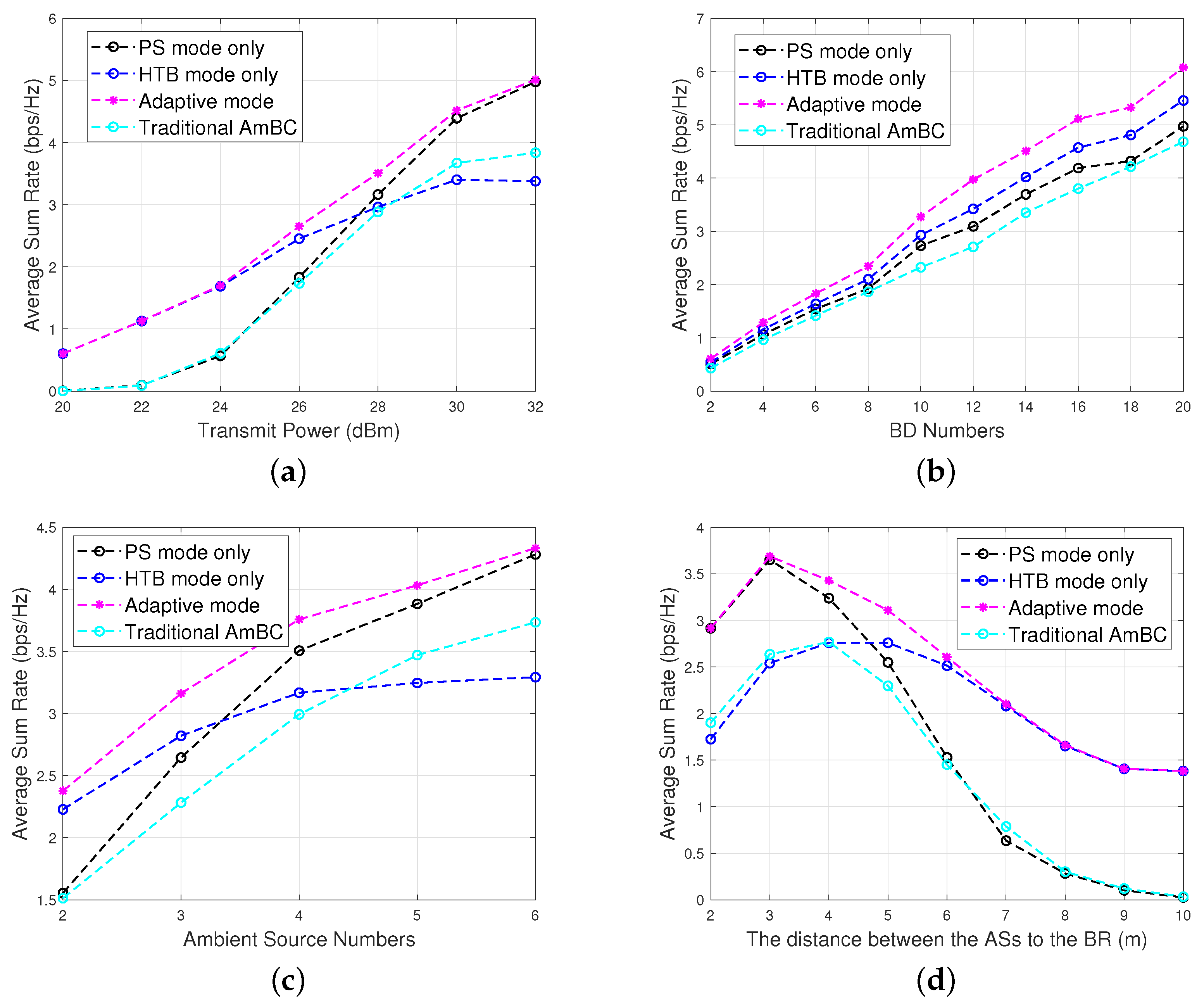
• To validate the outage probability and sun rate performance of our proposed adaptive strategy, extensive simulations compare them with non-adaptive transmission in massive IoT networks. The simulation results highlight the superior stability and efficiency of our proposed scheme in multi-AS and multi-BD AmBC systems. Our proposed low-power adaptive AmBC can achieve a 34.8% average sum rate performance improvement compared to a traditional AmBC with a common setup, i.e., 27 dBm transmit power, 10 BDs, three ASs, and 5 m distance between the ASs and the BR. Moreover, we have provided the mathematical derivation of the outage probabilities and conducted verification. The results confirm the accuracy and tightness of the derivations, where the error does not exceed 0.01.
• As for application scenarios, our proposed low-power adaptive strategy is particularly well suited for massive IoT involving multiple AS and multiple BD. For instance, it applies to scenarios with multiple ASs such as smart homes, as well as to smart agriculture and smart logistics where there are densely deployed passive BDs. In these scenarios, the method can enhance the network sum rate, ensure more stable connections, and reduce the outage probability, thereby enabling massive communication.

Notations: Bold lower and upper case letters denote vectors and matrices, respectively. Complex scalars are assumed, and their set is denoted by $\mathbb{C}$. The circularly symmetric complex Gaussian distribution with mean $\mu$ and variance ${\sigma }^2$ is $\mathcal{CN}(\mu ,{\sigma }^2)$. ${\mathbf{I}}_M$ denotes the $M\times M$ identity matrix. The Euclidean norm of a vector is $\parallel ·\parallel$, and the Frobenius norm of a matrix is ${\parallel ·\parallel }_F$. $\mathbb{E}[·]$ denotes statistical expectation.

2. System Model

We consider an adaptive multi-source AmBC system in massive IoT networks, consisting of K ambient sources (ASs), J single-antenna passive BDs, and a backscatter receiver (BR) equipped with M antennas, as shown in Figure 1. The ambient signal of the k-th AS is denoted by $\sqrt{P_k^S}{s}_k\left(n\right)$ with transmit power $P_k^S$. The normalized signal of the k-th AS in the n-th sample is denoted by $s_k\left(n\right)$ and is assumed to follow a circularly symmetric complex Gaussian (CSCG) distribution, i.e., $s_k\left(n\right)\sim \mathcal{CN}(0,1)$, since it is unpredictable to the BDs [21,22]. The BDs can operate in power-splitting (PS) mode and harvest-then-backscattering (HTB) mode, which depends on whether the BD can harvest sufficient energy from the AS signals via a designed decision threshold from the BR. If the j-th BD is in the PS mode, it splits ${\alpha }_j\in [0,1]$ power for backscattering and $(1-{\alpha }_j)$ power for energy harvesting simultaneously. Otherwise, in the HTB mode, it firstly allocates ${\tau }_j$ time duration for energy harvesting accumulation and then starts backscattering. The decision threshold is denoted by $p_{th}$, which will be specifically introduced in the following subsection. In addition, the BDs are equipped with an impedance network, which can provide an adjustable RC [13], i.e., $\alpha$. The M-antenna BR utilized the receive combining technique and maximum likelihood (ML) detection rule to demodulate backscatter symbols.

We assumed that all the channels are flat block fading channels and subject to path loss and Rayleigh fading [13,23]. The channels can be regarded as constant during a channel coherent interval (CCI), and they change independently among different intervals. We assume the CCI is no less than one transmit slot T, as shown in Figure 2. For the sake of fairness, each BD occupies $T/J$ time duration for its backscatter communication. Let ${\mathbf{g}}_k={[g_{k,1},g_{k,2},\dots ,g_{k,M}]}^T\in {\mathbb{C}}^{M\times 1},f_{k,j}\in \mathbb{C},{\mathbf{h}}_j={[h_{j,1},h_{j,2},\dots ,h_{j,M}]}^T\in {\mathbb{C}}^{M\times 1}$ denote the channel coefficients of the direct link from the k-th AS to the BR, the forward link from the k-th AS to the j-th BD, and the backward link from the j-th BD to the BR, respectively. We assume all the channels follow an independent and identical (i.i.d) Rayleigh distribution, i.e., $f_{k,j}\sim \mathcal{CN}(0,{\sigma }_{f_{k,j}}^2)$, $g_{k,m}\sim \mathcal{CN}(0,{\sigma }_{g_{k,m}}^2)$, and $h_{j,m}\sim \mathcal{CN}(0,{\sigma }_{h_{j,m}}^2)$, where $m=1,2,\dots ,M$ is the index of the receive antenna at the BR. ${\sigma }_{f_{k,j}}^2,{\sigma }_{g_{k,m}}^2$, and ${\sigma }_{h_{j,m}}^2$ are their overall channel gains, respectively, which can be calculated by the Friis Equation as

$${\sigma }_{f_{k,j}}^2={\displaystyle \frac{G_k^S{G}_j^T{\lambda }^2}{{\left(4\pi \right)}^2{L}_{f_{k,j}}^{{\nu }_f}}},{\sigma }_{g_{k,m}}^2={\displaystyle \frac{G_k^S{G}_m^R{\lambda }^2}{{\left(4\pi \right)}^2{L}_{g_{k,m}}^{{\nu }_g}}},{\sigma }_{h_{j,m}}^2={\displaystyle \frac{G_j^T{G}_m^R{\lambda }^2}{{\left(4\pi \right)}^2{L}_{h_{j,m}}^{{\nu }_h}}},$$

(1)

where $G_k^S,G_j^T,G_m^R$ are the antenna gains of the k-th AS, the j-th BD, and the m-th receive antenna at the BR, respectively. $\lambda$ is the wavelength of the ambient signals. $L_{f_{k,j}},L_{g_{k,m}},L_{h_{j,m}}$ are the distance between the k-th AS and the j-th BD, the distance between the k-th AS and the m-th receive antenna, and the distance between the j-th BD and the m-th receive antenna, respectively. ${\nu }_f,{\nu }_g,{\nu }_h$ are the path loss exponents of the forward link, direct link, and backscatter link, respectively.

2.1. Low-Power Adaptive Strategy

Consider there are J passive BDs waiting for data backscattering in the t-th transmit slot, as shown in Figure 2. When the BDs can harvest enough power, the BDs use PS mode to backscatter while harvesting. Under some channel conditions, the passive BDs cannot harvest enough power where the HTB mode will be adopted to store little energy before backscatter. In this way, the outage probability of AmBC can be reduced. However, the backscatter data rate will also be reduced since a part of the transmit slot is utilized to accumulate harvested energy. There exists a trade-off between outage probability and data rate. In this subsection, we propose a low-power adaptive strategy, which can balance the above performances via assigning a local decision threshold to the passive BDs, avoiding extra communications between the BDs and the BR. The details are as follows:

• As a central device, the BR globally divides the J BDs into two subsets, $J_1$ and $J_2$, by designing a decision threshold $p_{th}$. Specifically, the BR assigns the decision threshold to the J BDs. The BDs in $J_1$, which can harvest more than $p_{th}$ power, locally decide that they are supposed to adopt PS mode. The others, in $J_2$, which cannot harvest sufficient power, adopt HTB mode. By assigning the appropriate $p_{th}$, the BR can easily balance the outage probability and sum data rate performance of the J BDs while the passive BDs are insensitive to decision changes. To further boost the adaptive strategy by achieving a maximum sum data rate while ensuring power supply constraints, the BR jointly designs optimal RCs ${\left\{{\alpha }_j\right\}}_{j\in J_1}$ for the BDs in $J_1$, optimal harvest accumulation time duration ${\left\{{\tau }_j\right\}}_{j\in J_2}$, and optimal RC ${\left\{{\beta }_j\right\}}_{j\in J_2}$ via solving a sum rate maximization problem.
• At the passive BDs, they can receive the decision threshold $p_{th}$ from the BR using an analog circuit, as in [4,24], and compare their harvested power strength with $p_{th}$. In the PS backscatter mode, the transmit frame includes a training period and a data transmission period, as shown in Figure 2. They adjust their RC ${\alpha }_j(j\in J_1)$ to backscatter ambient signals as much as possible while guaranteeing their minimum circuit operating energy. In the HTB backscatter mode, the BDs first harvest energy in the ${\tau }_j(j\in J_2)$ time period before backscattering to satisfy their minimum circuit operating energy, as shown in Figure 2. Different from the traditional HTT protocol, which makes an active transmission, the BD in HTB mode still adopts backscatter communication with an RC ${\beta }_j(j\in J_2)$ since it is a passive device without any active RF components.

2.2. Signal Model

2.2.1. Direct-Link Interference Signal

Consider the system model in Figure 1, the direct-link signals come from the K ASs to the BR, directly. The received signal at the m-th antenna of the BR from the k-th AS can be given by

$$y_{k,m}^{SR}=\sqrt{P_k^S}{g}_{k,m}{s}_k\left(n\right),$$

(2)

and the entire signal from K ASs at the m-th receive antenna is expressed as

$$y_m^{SR}=\sum _{k=1}^K{y}_{k,m}^{SR}=\sum _{k=1}^K\sqrt{P_k^S}{g}_{k,m}{s}_k\left(n\right).$$

(3)

Then, the vector form of the received direct-link interference signal is given by

$${\mathbf{y}}^{SR}={[y_1^{SR},y_2^{SR},\dots ,y_M^{SR}]}^T=\sum _{k=1}^K\sqrt{P_k^S}{\mathbf{g}}_k{s}_k\left(n\right)\in {\mathbb{C}}^{M\times 1}.$$

(4)

2.2.2. Cascaded Forward-Link and Backscatter-Link Signals

The forward-link received signal at the j-th BD from the k-th AS denoted by $y_{k,j}^{ST}$ is expressed as

$$y_{k,j}^{ST}=\sqrt{P_k^S}{f}_{k,j}{s}_k\left(n\right),$$

(5)

where the received noise at the BD can be ignored since the BDs are passive devices [3,23,24]. Thus, the overall forward-link received signals at the j-th BD is given by

$$y_j^{ST}=\sum _{k=1}^K{y}_{k,j}^{ST}=\sum _{k=1}^K\sqrt{P_k^S}{f}_{k,j}{s}_k\left(n\right).$$

(6)

The RF-EH efficiency of the BDs is assumed as $\eta$. Thus, the harvested power by the j-th BD can be derived as

$$P_j^T=\eta \sum _{k=1}^K{P}_k^S|f_{k,j}{|}^2\mathbb{E}\left[\right|s_k{\left(n\right)|}^2]=\eta \sum _{k=1}^K{P}_k^S{\left|f_{k,j}\right|}^2,$$

(7)

where $\mathbb{E}\left[\right|s_k\left(n\right){|}^2]=1$ because $s_k\left(n\right)\sim \mathcal{CN}(0,1)$.

Accordingly, when $P_j^T$ is higher than the decision threshold $p_{th}$, the j-th BD uses the PS mode to realize simultaneous RF-EH and backscatter communication. When $P_j^T$ is lower than $p_{th}$, the j-th BD adopts the HTB mode to harvest energy first, before backscatter communication. The signal models of the above two cases are analyzed as follows:

Case 1:$P_j^T\ge p_{th}$ (PS mode). The BD uses the PS frame as shown in Figure 2. Consider the j-th BD, in the whole backscatter transmission period $T/J$, the BD splits ${\alpha }_j$ received ambient signals for backscattering while the remaining $(1-{\alpha }_j)$ received ambient signals for RF-EH. They can adjust their RCs by switching to different load impedances in the impedance network. Therefore, the harvested power used for on-BD circuit operation is given by

$$P_j^{T,PS}=(1-{\alpha }_j)P_j^T\ge P_c,$$

(8)

where $P_c$ is the minimum on-BD circuit operation power.

At the same time, the received signal at the j-th BD for backscatter communication can be written as

$$y_j^{T,PS}={\alpha }_j{y}_j^{ST}.$$

(9)

Accordingly, the received signal at the m-th BR antenna from the cascaded backscatter link from the j-th BD is given by

$$y_{j,m}^{TR,PS}=y_j^{T,PS}{h}_{j,m}{x}_j={\alpha }_j\sum _{k=1}^K\sqrt{P_k^S}{f}_{k,j}{h}_{j,m}{x}_j{s}_k\left(n\right),$$

(10)

where $x_j$ is the backscatter symbol of the j-th BD who adopts OOK load modulation, i.e., $x_j\in \{0,1\}$. Then, the vector form of the received backscatter signal of the j-th BD at the BR is written as

$${\mathbf{y}}_j^{TR,PS}={[y_{j,1}^{TR,PS},y_{j,2}^{TR,PS},\dots ,y_{j,M}^{TR,PS}]}^T={\alpha }_j\sum _{k=1}^K\sqrt{P_k^S}{f}_{k,j}{\mathbf{h}}_j{x}_j{s}_k\left(n\right)\in {\mathbb{C}}^{M\times 1}.$$

(11)

Case 2:$P_j^T<p_{th}$ (HTB mode). The BD uses the HTB frame as shown in Figure 2. Before the backscatter transmission, the j-th BD first harvests RF power in the time duration ${\tau }_j$. Then, it backscatters the incident ambient signals in the remaining $({\displaystyle \frac{T}{J}}-{\tau }_j)$ time duration with RC ${\beta }_j$. The total harvested energy used for on-BD circuit operation is

$$E_j^{T,HTB}=(1-{\beta }_j)P_j^T\left[{\tau }_j+({\displaystyle \frac{T}{J}}-{\tau }_j)\right]=P_j^{T,HTB}{\displaystyle \frac{T}{J}}\ge P_c({\displaystyle \frac{T}{J}}-{\tau }_j),$$

(12)

and the received signal at the j-th BD used for backscattering is

$$y_j^{T,HTB}={\beta }_j{y}_j^{ST}.$$

(13)

Accordingly, the received signal at the m-th BR antenna from the cascaded backscatter link from the j-th BD in HTB mode is given by

$$y_{j,m}^{TR,HTB}=y_j^{T,HTB}{h}_{j,m}{x}_j={\beta }_j\sum _{k=1}^K\sqrt{P_k^S}{f}_{k,j}{h}_{j,m}{x}_j{s}_k\left(n\right).$$

(14)

Then, the vector form of the received backscatter signal of the j-th BD at the BR is written as

$${\mathbf{y}}_j^{TR,HTB}={[y_{j,1}^{TR,HTB},y_{j,2}^{TR,HTB},\dots ,y_{j,M}^{TR,HTB}]}^T={\beta }_j\sum _{k=1}^K\sqrt{P_k^S}{f}_{k,j}{\mathbf{h}}_j{x}_j{s}_k\left(n\right)\in {\mathbb{C}}^{M\times 1}.$$

(15)

2.2.3. Overall Superposed Signal

Substituting (4), (11), and (15), the vector form of received signals at the BR for PS mode and HTB mode can be expressed as

$${\mathbf{y}}_j^{PS}\left(n\right)={\mathbf{y}}^{SR}\left(n\right)+{\mathbf{y}}_j^{TR,PS}\left(n\right)+\mathbf{u}\left(n\right),$$

(16)

and

$${\mathbf{y}}_j^{HTB}\left(n\right)={\mathbf{y}}^{SR}\left(n\right)+{\mathbf{y}}_j^{TR,HTB}\left(n\right)+\mathbf{u}\left(n\right),$$

(17)

respectively, where $\mathbf{u}\left(n\right)\sim \mathcal{CN}(0,{\sigma }^2{\mathbf{I}}_M)$ is the additive Gaussian white noise (AWGN) matrix. Considering that the BR uses the receive combining technique [21,25] and ML detection rule [3,22] to detect the backscatter symbol $x_j$, we assume the combining vector is denoted by $\mathbf{w}\in {\mathbb{C}}^{M\times 1}$, where ${\parallel \mathbf{w}\parallel }^2=1$. For simplicity, in this paper, we take $\mathbf{w}={[0.5,0.5,0.5,0.5]}^T$. Thus, the combined signal received at the BR antenna is expressed as

$$y_j^i\left(n\right)={\mathbf{w}}^H{\mathbf{y}}_j^i\in \mathbb{C},i\in \{PS,HTB\}.$$

(18)

Substituting (16) and (17) into (18), we have

$$y_j^{PS}\left(n\right)=\sum _{k=1}^K\sqrt{P_k^S}{\mathbf{w}}^H({\mathbf{g}}_k+\alpha f_{k,j}{\mathbf{h}}_j{x}_j)s_k\left(n\right)+{\mathbf{w}}^H\mathbf{u}\left(n\right),$$

(19)

and

$$y_j^{HTB}\left(n\right)=\sum _{k=1}^K\sqrt{P_k^S}{\mathbf{w}}^H({\mathbf{g}}_k+{\beta }_j{f}_{k,j}{\mathbf{h}}_j{x}_j)s_k\left(n\right)+{\mathbf{w}}^H\mathbf{u}\left(n\right),$$

(20)

respectively.

Therefore, the signal-to-interference-and-noise ratio (SINR) of the backscatter signal at the PS mode is written as

$${\gamma }_j^{PS}={\displaystyle \frac{{\sum }_{k=1}^K{\alpha }_j{P}_k^S|f_{k,j}{|}^2{|{\mathbf{w}}^H{\mathbf{h}}_j|}^2}{{\sum }_{k=1}^K{P}_k^S{\left|{\mathbf{w}}^H{\mathbf{g}}_k\right|}^2+{\sigma }^2}},$$

(21)

and

$${\gamma }_j^{HTT}={\displaystyle \frac{{\sum }_{k=1}^K{\beta }_j{P}_k^S|f_{k,j}{|}^2{|{\mathbf{w}}^H{\mathbf{h}}_j|}^2}{{\sum }_{k=1}^K{P}_k^S{\left|{\mathbf{w}}^H{\mathbf{g}}_k\right|}^2+{\sigma }^2}},$$

(22)

respectively.

2.3. Problem Formulation

According to the protocol in Figure 2, the sum backscatter data rate can be given by

$$\mathcal{R}=\underset{{\mathcal{R}}_1}{\underbrace{{\displaystyle \frac{T}{J}}\sum _{j=1}^{J_1}{log}_2(1+{\gamma }_j^{PS})}}+\underset{{\mathcal{R}}_2}{\underbrace{\sum _{j=1}^{J_2}({\displaystyle \frac{T}{J}}-{\tau }_j){log}_2(1+{\gamma }_j^{HTB})}}.$$

(23)

Notation: The transmit time durations ${\displaystyle \frac{T}{J}}$ and ${\displaystyle \frac{T}{J}}-{\tau }_j$ are considered in $\mathcal{R}$ for the sake of convenience. Actually, we can obtain a sum rate in the traditional sense by calculating $\mathcal{R}/(T/J)$.

Therefore, we propose the following sum rate maximization problem as

$$\begin{array}{cc}\hfill \mathit{P}\mathbf{1}:& \underset{p_{th},{\alpha }_j,{\tau }_j,{\beta }_j}{max}\mathcal{R},\hfill \end{array}$$

(24)

$$\begin{array}{cc}\hfill s.t.& j\in J_1,P_j^T\ge p_{th}\hfill \end{array}$$

(24a)

$$\begin{array}{cc}\hfill & j\in J_2,P_j^T<p_{th}\hfill \end{array}$$

(24b)

$$\begin{array}{cc}\hfill & P_j^{T,PS}\ge P_c,j\in J_1\hfill \end{array}$$

(24c)

$$\begin{array}{cc}\hfill & E_j^{T,HTB}\ge P_c({\displaystyle \frac{T}{J}}-{\tau }_j),j\in J_2\hfill \end{array}$$

(24d)

$$\begin{array}{cc}\hfill & 0\le {\tau }_j\le {\displaystyle \frac{T}{J}},j\in J_2\hfill \end{array}$$

(24e)

$$\begin{array}{cc}\hfill & {\alpha }_j,{\beta }_j\in [0,1],j\in J\hfill \end{array}$$

(24f)

$$\begin{array}{cc}\hfill & J_1+J_2=J\hfill \end{array}$$

(24g)

where (24a,b) are the low-power adaptive strategy for user scheduling. (24c) is the on-BD circuit operation power constraint of the BDs in PS mode. (24d) is the RF-EH constraint of the BDs in HTB mode using time duration allocation. (24e–g) are the constraints of variables ${\tau }_j$, ${\alpha }_j$, ${\beta }_j$,$J_1$, and $J_2$. The problem is non-convex and complex due to the coupling between the problem and its constraints.

3. Solution to the Sum Rate Maximization Problem

The proposed sum rate maximization problem is quite complicated and untraceable. In this section, we first decompose the aforementioned optimal problem into several subproblems, i.e., the RC optimization problem, the time allocation problem, and the user scheduling problem. These subproblems decouple the constraints, making the problem solvable. Additionally, by relaxing the variables problem, we make the user scheduling traceable.

3.1. RC Optimization

Consider the BDs in $J_1$, the subproblem of maximizing ${\mathcal{R}}_1$ in (23) via ${\left\{{\alpha }_j\right\}}_{j\in J_1}$ is proposed. Since only the constraints (24c) and (24f) are related to RC, we conduct the subproblem $\mathbf{P}\mathbf{2}$ as   

$$\begin{array}{cc}\hfill \mathit{P}\mathbf{2}:& \underset{{\alpha }_j}{max}\sum _{j=1}^{J_1}{log}_2(1+{\gamma }_j^{PS}),\hfill \end{array}$$

(25)

$$\begin{array}{cc}\hfill s.t.& P_j^{T,PS}\ge P_c,j\in J_1\hfill \end{array}$$

(25a)

$$\begin{array}{cc}\hfill & {\alpha }_j\in [0,1]\hfill \end{array}$$

(25b)

where $P_j^{T,PS}=(1-{\alpha }_j)\eta {\sum }_{k=1}^K{P}_k^S{\left|f_{k,j}\right|}^2$, which is expanded by substituting (7) into (8). (25a) is the on-BD circuit operation power constraint of the BDs in PS mode. (25b) refers to the definition range of ${\alpha }_j$.

Since ${\alpha }_j$ is independent for each BD in $J_1$ and the logarithmic function in (25) is monotonically increasing, the maximum of $\mathbf{P}\mathbf{2}$ is derived when each ${\gamma }_j^{PS}$ reaches its maximum. According to [13,26], we have the solution of ${\alpha }_j^{*}$ given by

$${\alpha }_j^{*}=max\left(0,1-{\displaystyle \frac{P_c}{\eta {\sum }_{k=1}^K{P}_k^S{\left|f_{k,j}\right|}^2}}\right).$$

(26)

3.2. Time Allocation

Consider the BDs in $J_2$, the subproblem of maximizing ${\mathcal{R}}_2$ in (23) via ${\left\{{\tau }_j\right\}}_{j\in J_2}$ and ${\left\{{\beta }_j\right\}}_{j\in J_2}$ is proposed as the subproblem $\mathbf{P}\mathbf{3}$

$$\begin{array}{cc}\hfill \mathit{P}\mathbf{3}:& \underset{{\tau }_j,{\beta }_j}{max}\sum _{j=1}^{J_2}({\displaystyle \frac{T}{J}}-{\tau }_j){log}_2(1+{\gamma }_j^{HTB}),\hfill \end{array}$$

(27)

$$\begin{array}{cc}\hfill s.t.& (1-{\beta }_j)P_j^T{\displaystyle \frac{T}{J}}\ge P_c({\displaystyle \frac{T}{J}}-{\tau }_j),j\in J_2\hfill \end{array}$$

(27a)

$$\begin{array}{cc}\hfill & 0\le {\tau }_j\le {\displaystyle \frac{T}{J}}\hfill \end{array}$$

(27b)

$$\begin{array}{cc}\hfill & {\beta }_j\in [0,1],j\in J_2\hfill \end{array}$$

(27c)

where (27a) is derived from (12) and (24d), which is an RF-EH power constraint that must meet the following on-BD operation power consumption when backscattering. (27b) and (27c) are the definition range of ${\tau }_j$ and ${\beta }_j$. This subproblem is the same as $\mathbf{P}\mathbf{2}$, which is a sum of $J_2$ independent monotonically increasing logarithmic functions. To ensure the on-BD circuit operation energy constraint (27a), we first fix variable ${\beta }_j$ and we obtain the solution to ${\tau }_j$ as

$${\tau }_j^{*}=max\left(0,{\displaystyle \frac{T}{J}}({\displaystyle \frac{P_c-(1-{\beta }_j)P_j^T}{P_c}})\right).$$

(28)

Then, substituting (28) into (29), we have the following problem

$$\begin{array}{cc}\hfill \mathit{P}{\mathbf{3}}^{\prime }:& \underset{{\beta }_j}{max}\sum _{j=1}^{J_2}{\displaystyle \frac{T}{J}}{\displaystyle \frac{(1-{\beta }_j)P_j^T}{P_c}}{log}_2(1+{\beta }_j{\overline{\gamma }}_j^{HTB}),\hfill \end{array}$$

(29)

$$\begin{array}{cc}\hfill s.t.& {\beta }_j\in [0,1],j\in J_2\hfill \end{array}$$

(29a)

where

$${\overline{\gamma }}_j^{HTB}={\displaystyle \frac{{\sum }_{k=1}^K{P}_k^S|f_{k,j}{|}^2{|{\mathbf{w}}^H{\mathbf{h}}_j|}^2}{{\sum }_{k=1}^K{P}_k^S{\left|{\mathbf{w}}^H{\mathbf{g}}_k\right|}^2+{\sigma }^2}},$$

(30)

and the problem in $\mathbf{P}{\mathbf{3}}^{\prime }$ is a sum of $J_2$ independent concave functions. (29a) is the definition range of ${\beta }_j$. The close-form of the solution to the concave function $f\left(x\right)=(1-x){log}_2(1+ax),a>0,x\in [0,1]$ is easy to be solved. The maximum value is given by

$${\beta }_j^{*}={\displaystyle \frac{exp\left({\mathcal{W}}_0(e{\overline{\gamma }}_j^{HTT}+e)-1\right)-1}{{\overline{\gamma }}_j^{HTT}}}\in [0,1].$$

(31)

where ${\mathcal{W}}_0(·)$ is the principal branch of the Lambert W function.

3.3. User Scheduling

When it comes to $p_{th}$, the problem becomes untraceable since the variables $J_1$ and $J_2$ are discrete and we need to exhaustive search subset combinations of $J_1$ and $J_2$.

Substituting the optimal RC ${\alpha }_j^{*}$, optimal time allocation ${\tau }_j^{*}$ and ${\beta }_j^{*}$ to problem $\mathbf{P}\mathbf{1}$, we conduct $p_{th}$ to schedule the J BDs into subset $J_1$ or $J_2$, according to the low-power adaptive strategy in Section 2.1. Thus, we have the subproblem $\mathbf{P}\mathbf{4}$ as

$$\begin{array}{cc}\hfill \mathit{P}\mathbf{4}:& \underset{p_{th}}{max}{\displaystyle \frac{T}{J}}\sum _{j=1}^{J_1}{log}_2(1+{\gamma }_j^{PS}{|}_{{\alpha }_j^{*}})+\sum _{j=1}^{J_2}\left({\displaystyle \frac{T}{J}}-{\tau }_j^{*}\right){log}_2(1+{\gamma }_j^{HTB}{|}_{{\beta }_j^{*}}),\hfill \end{array}$$

(32)

$$\begin{array}{cc}\hfill s.t.& j\in J_1,P_j^T\ge p_{th},\hfill \end{array}$$

(32a)

$$\begin{array}{cc}\hfill & j\in J_2,P_j^T<p_{th},\hfill \end{array}$$

(32b)

$$\begin{array}{cc}\hfill & J_1+J_2=J\hfill \end{array}$$

(32c)

where (32a) and (32b) are the definition sets of j, and (32c) is the relationship between $J_1$ and $J_2$.

The subproblem $P4$ is a discrete programming problem of set J. To make it traceable, we introduce a continuous variable to solve it. Assume the probability of the BD in the $J_1$ is ${\theta }_j$, where ${\theta }_j\in [0,1]$. Then, its probability in the subset $J_2$ is $(1-{\theta }_j)$. Thus, the subproblem $\mathbf{P}\mathbf{4}$ can be expressed as

$$\begin{array}{cc}\hfill \mathit{P}{\mathbf{4}}^{\prime }:& \underset{{\theta }_j}{max}{\displaystyle \frac{T}{J}}\sum _{j=1}^J{\theta }_j{log}_2(1+{\gamma }_j^{PS}{|}_{{\alpha }_j^{*}})+\sum _{j=1}^J(1-{\theta }_j)\left({\displaystyle \frac{T}{J}}-{\tau }_j^{*}\right){log}_2(1+{\gamma }_j^{HTB}{|}_{{\beta }_j^{*}}),\hfill \end{array}$$

(33)

$$\begin{array}{cc}\hfill s.t.& {\theta }_j=0,P_j^T<P_c\hfill \end{array}$$

(33a)

$$\begin{array}{cc}\hfill & {\theta }_j\in [0,1]\hfill \end{array}$$

(33b)

where the constraint (33a) guarantees the power constraint of the BDs in PS mode. (33b) is the definition range of ${\theta }_j$.

The above subproblem is traceable and convex, which can be solved by the CVX Tool (v2.2). To recover the subset $J_1$ and $J_2$, we propose the following rule

$${\theta }_j^{*}=\left\{\begin{array}{c}1,{\theta }_j\ge {\displaystyle \frac{1}{2}},\hfill \\ 0,\mathrm{otherwise}.\hfill \end{array}\right.$$

(34)

After that, we have the division of the subsets $J_1$ and $J_2$. The decision threshold can be conducted by

$$p_{th}^{*}=min\left(P_j^T\right),j\in J_1.$$

(35)

As a summary of the step-by-step solution for the above algorithm, the pseudocode is given by Algorithm 1.

Algorithm 1 Joint optimizing method for the sum rate maximization problem

Input: channel gains: $|f_{k,j}{|}^2$, $|{\mathbf{w}}^H{\mathbf{h}}_j{|}^2$ and $|{\mathbf{w}}^H{\mathbf{g}}_k{|}^2$, which can be estimated as [27,28,29] using training symbols in training period as shown in Figure 2   1: Calculate ${\alpha }_j^{*}$ by solving (25).   2: Calculate ${\tau }_j^{*}$,${\beta }_j^{*}$ by solving (27) and (29).   3: Optimize ${\theta }_j^{*}$ by substituting ${\alpha }_j^{*}$, ${\tau }_j^{*}$ and ${\beta }_j^{*}$ into (33).   4: Obtain subset $J_1$ and $J_2$ by convert ${\theta }_j^{*}$ into a discrete value according to the rule (34).   5: Obtain $p_{th}^{*}$ by (35). Output: $p_{th}^{*}$

Complexity analysis: The computational complexity of calculating ${\alpha }_j^{*}$, ${\tau }_j^{*}$ and ${\beta }_j^{*}$ is $\mathcal{O}\left(1\right)$, since they have closed-form solutions. The computational complexity of optimizing ${\theta }_j^{*}$ depends on the CVX Tools, and it is proportional to the number of BDs, i.e., $\mathcal{O}\left(J\right)$. The computation complexity of converting ${\theta }_j^{*}$ and obtaining $p_{th}^{*}$ is obviously $\mathcal{O}\left(1\right)$.

4. Outage Probability Analysis for Multi-Source AmBC

In this section, we derive the theoretical outage probability analysis for the BDs in multi-source AmBC using PS mode and HTB mode, respectively.

4.1. Outage Probability of the j-th BD Using PS Mode

To analyze the outage probability of our proposed low-power multi-AS multi-BD AmBC system, we recall the harvested power in (7) and the signal model in (18). In PS mode, the outage occurs when the harvested power is less than the minimum circuit operation power $P_c$ or the received SINR is less than the SINR threshold ${\gamma }_0$, though the harvested power is sufficient. Thus, the outage probability of the j-th BD using PS mode is given by

$${\mathcal{P}}_j^{out,PS}=\underset{{\mathcal{I}}_1}{\underbrace{\mathbb{P}(P_j^T<P_c)}}+\underset{{\mathcal{I}}_2}{\underbrace{\mathbb{P}({\gamma }_j^{PS}<{\gamma }_0,P_j^T\ge P_c)}}.$$

(36)

To obtain the numerical formula, we calculate integrations ${\mathcal{I}}_1$ and ${\mathcal{I}}_2$, respectively.

Theorem 1. 

Calculate the cumulative distribution function (CDF) of $P_j^T/\eta$.

To calculate the above CDF, we need to consider the random variables (RVs) in $P_j^T$, i.e., $|f_{k,j}{|}^2$ first. Consider the formula $P_j^T$ in (7); it is a linear combination of K independent exponential random variable, i.e., $|f_{k,j}{|}^2\sim exp(1/{\lambda }_{f_{k,j}}^2)$, where the parameter ${\lambda }_{f_{k,j}}={\sigma }_{f_{k,j}}^2$, for the sake of convenience in notation. The CDF of $P_j^T/\eta$ in (36) is given by

$$F_{{\lambda }_{f_j}}\left(x\right)=1-\sum _{k=1}^K{A}_{k}exp(-{\displaystyle \frac{x}{P_k^S{\lambda }_{f_{k,j}}}}).$$

(37)

Proof of Theorem 1. 

See Appendix A. □

Therefore, integration ${\mathcal{I}}_1$ can be calculated according to Theorem 1 as follows

$$\begin{array}{cc}{\mathcal{I}}_1=& \mathbb{P}(P_j^T<P_c)\hfill \\ =& \mathbb{P}({\displaystyle \frac{P_j^T}{\eta }}<{\displaystyle \frac{P_c}{\eta }})\hfill \\ =& F_{{\lambda }_{f_j}}({\displaystyle \frac{P_c}{\eta }})=1-{\displaystyle \sum _{k=1}^K}{A}_{k}exp(-{\displaystyle \frac{P_c}{\eta P_k^S{\lambda }_{f_{k,j}}}}),\hfill \end{array}$$

(38)

where $A_k$ is given in (A4).

Theorem 2. 

The Integration of ${\mathcal{I}}_2$ is quite difficult to be calculated. In this paper, we derive an approximate close-form formula as

$${\mathcal{I}}_2\approx \sum _{k=1}^K\sum _{s=1}^K{\displaystyle \frac{A_k{B}_s\sqrt{P_k^S{P}_s^S{\gamma }_0{\lambda }_{g_k}{\lambda }_{f_{s,j}}}}{\sqrt{{\lambda }_{h_j}}}}exp\left({\displaystyle \frac{P_k^S{\lambda }_{g_k}{\gamma }_0}{2P_s^S{\lambda }_{h_j}{\lambda }_{f_{s,j}}}}\right)W_{-{\displaystyle \frac{1}{2}},0}\left({\displaystyle \frac{P_k^S{\lambda }_{g_k}{\gamma }_0}{P_s^S{\lambda }_{h_j}{\lambda }_{f_{s,j}}}}\right)+(1-{\mathcal{I}}_1)F_{b_j}\left({\sigma }^2{\gamma }_0\right),$$

(39)

where $B_s$ is given in (A5). $F_{b_j}(·)$ is expressed as (A6). $W_{-{\displaystyle \frac{1}{2}},0}(·)$ is the Whittaker functions.

Proof of Theorem 2. 

See Appendix C. □

Thus, the outage probability of the BDs in PS mode ${\mathcal{P}}_j^{out,PS}$ is derived by substituting (38) and (39).

4.2. Outage Probability of the j-th BD Using HTB Mode

As for the BDs in $J_2$ which adopt HTB mode, we assume that they can always guarantee power supply for the incoming backscatter. The reason is that if the j-th BD cannot harvest enough energy for backscattering, the ${\tau }_j$ will be ${\displaystyle \frac{T}{J}}$, which means that there remains no time duration for backscattering. It is impossible for the HTB protocol. Thus, the outage probability of the BDs in HTB mode can be expressed as

$${\mathcal{P}}_j^{out,HTT}=\mathbb{P}({\gamma }_j^{HTT}<{\gamma }_0).$$

(40)

Theorem 3. 

As for (40), it is likely to be ${\mathcal{I}}_2$. Alternatively, the outage probability ${\mathcal{P}}_j^{out,HTB}$ is a total probability, whereas ${\mathcal{I}}_2$ is a joint probability. Similarly, it can be given by

$$\mathbb{P}({\gamma }_j^{HTT}<{\gamma }_0)\approx \sum _{k=1}^K\sum _{s=1}^K{\displaystyle \frac{A_k{B}_s^{\prime }\sqrt{P_k^S{P}_s^S{\gamma }_0{\lambda }_{g_k}{\lambda }_{f_{s,j}}}}{\sqrt{{\beta }_j^{*}{\lambda }_{h_j}}}}exp\left({\displaystyle \frac{P_k^S{\lambda }_{g_k}{\gamma }_0}{2P_s^S{\beta }_j^{*}{\lambda }_{h_j}{\lambda }_{f_{s,j}}}}\right)W_{-{\displaystyle \frac{1}{2}},0}\left({\displaystyle \frac{P_k^S{\lambda }_{g_k}{\gamma }_0}{P_s^S{\beta }_j^{*}{\lambda }_{h_j}{\lambda }_{f_{s,j}}}}\right).$$

(41)

Proof of Theorem 3. 

See Appendix D. □

5. Numerical and Simulation Results

In this section, we provide simulations to validate the performance of our proposed low-power adaptive strategy and the theoretical analysis of the outage probabilities. The number of ASs is $K=3$, and the number of BDs is $J=10$. We set the power of the AS signal as 30 dBm, with a frequency of 915 MHz, which is 5 m away from the BR. The distances between the BDs and BR are about 0.1–0.2 m. We assume ${\mathbf{g}}_k,f_{k,j},{\mathbf{h}}_j$ are Rayleigh fading channels, and the power strengths of these channels are decided by path loss according to the Friis formula [3]. The antenna gains of the ASs and the BR are set as 4 dBi [30]. The antenna gains of the BDs are 1.2 dBi [31]. The path loss exponents are ${\nu }_f=2$, ${\nu }_g=3$ and ${\nu }_h=3$. The RF-EH efficiency of the BDs is $\eta =0.6$ [32]. The basic BD operation power is $P_c$ = 100 μW [30]. We conducted the numeric simulation experiments using extensive 10,000 Monte Carlo simulations.

In Figure 3, the comprehensive average sum rate performances of the proposed low-power adaptive strategy compared with traditional AmBC systems [3,4,5,6,7,8,9], as well as schemes only in PS mode [13,14,15,16] and HTB mode [10,11,12,19], are simulated. In Figure 3a, the average sum rate performances versus the transmit power ranging from 20 to 32 dBm are evaluated with K = 3 and J = 10. All modes increase with the increase in transmit power, and the result shows that our proposed adaptive mode can always achieve the best performance compared to the other two adaptive modes and traditional AmBC systems [3,4,5,6,7,8,9]. As can be observed, the adaptive mode is actually a linear combination of the PS mode and HTB mode. Therefore, the adaptive mode prefers the HTB mode when the transmit power is low and prefers the PS mode when the transmit power is high. The proposed adaptive method always achieves an average of about 1 bps/Hz sum rate gain compared with the traditional AmBC. At 27 dBm, the proposed adaptive method achieves about 34.8% gain. Figure 3b compares the average sum rate performances versus the number of BDs with 27dBm transmit power, K = 3, J = 10. It is obvious that more BDs can reach a higher sum rate, and the adaptive mode achieves the best among all modes. Compared to traditional AmBC systems and the other two adaptive modes, i.e., PS mode only works in [13,14,15,16] and HTT/HTB mode only works in [10,11,12,19], the proposed adaptive method can achieve about 34.8%, 19.9%, and 11.8% average sum rate gain, respectively, when the BD number J is 10. Figure 3c illustrates the impact of ambient source numbers on the average sum rate performance with J = 10, 30 dBm transmit power. It is similar to Figure 3a since the transmit power increases with the number of ASs. Our proposed adaptive method and the PS mode only scheme comprehensively outperform traditional AmBC systems. However, compared to the HTB scheme, the traditional AmBC performs better when the number of signal sources exceeds four. This is because an increase in the number of sources can better guarantee the RF-EH performance of the passive BDs, which is beneficial for the PS mode. Figure 3d shows the relationship between the average sum rate and the AS-BR distances $d_{tr}$ with K = 3, J = 10, and 27 dBm transmit power. The result shows that the average sum rate achieves the best result when $d_{tr}=3$ m. When $d_{tr}<3$ m, the close ASs induce strong DLI to the BDs, causing the average sum rate to decrease. When $d_{tr}$ becomes large, the far ASs cannot provide sufficient power supply to the BDs. Furthermore, the proposed adaptive method outperforms other AmBC systems. Our work can achieve about 34.8% average sum rate gain when the $d_{tr}=5$ m compared to traditional AmBC systems [3,4,5,6,7,8,9], and the gains become larger with the increase in the $d_{tr}$.

In Figure 4, the numerical and simulation results of ${\mathcal{I}}_1$ are illustrated. (a) shows the simulated PDF and the theoretical PDF in Theorem 1. (b) compares the simulated outage probabilities and our derived ${\mathcal{I}}_1$ in (38) with K = 3, J = 10, 30 dBm transmit power, $\eta =0.6$ and $P_c=100$ μW, 200 μW, 300 μW. The results confirm the accuracy and tightness of our derivation of ${\mathcal{I}}_1$.

In Figure 5, the numerical and simulation results of ${\mathcal{I}}_2$ are illustrated. Figure 5a shows the simulated PDF and the theoretical PDF in the Appendix B.1. The results confirm the accuracy and tightness of our derivation of (A5). Figure 5b compares the simulated PDF and the approximate theoretical PDF in Appendix C. The figure shows that when x, i.e., SINR, is between about 1 and 5, the error comparison between them is significant. However, in AmBC, the DLI signal is generally 3–4 orders of magnitude higher than the weak backscatter signals [3], which means SINR ≪ 1, typically. Thus, our derived ${\mathcal{I}}_2$ is accurate for AmBC.

6. Conclusions

In this paper, we proposed an adaptive backscatter technique for multi-source AmBC. We introduced a low-power adaptive strategy for the AmBC system, where a decision threshold is assigned to passive BDs for selecting the appropriate backscatter mode. To enhance the system’s performance, we formulated a sum rate maximization problem that jointly optimizes the backscatter mode scheduling, RCs, and TA for passive BDs. Our proposed approach is validated through simulations, which demonstrate the significant improvements in sum rate and outage probability. The results also confirm the accuracy and effectiveness of the derived outage probabilities, proving the efficiency of the adaptive backscatter technique in real-world massive IoT applications. The findings suggest that the proposed method can provide reliable and energy-efficient backscatter communication, making it a promising solution for future IoT networks. In future work, we will consider grouping passive BDs with similar channel conditions in massive IoT scenarios and applying the proposed scheme to these grouped BDs to enhance the adaptability of the proposed low-power adaptive strategy, thereby broadening the applicability and efficiency of our approach. Moreover, studies incorporating physical platforms (e.g., testbeds and prototypes) should be conducted to further validate the effectiveness and practicality of our work.

References

1. Transforma Insights. IoT Connections Forecast 2023–2034. 2025. Available online: https://transformainsights.com/research/forecast/highlights (accessed on 9 March 2025).
2. Zhao, N.; Yu, F.R.; Sun, H.; Li, M. Adaptive power allocation schemes for spectrum sharing in interference-alignment-based cognitive radio networks. IEEE Trans. Veh. Technol. 2015, 65, 3700–3714. [Google Scholar] [CrossRef]
3. Van Huynh, N.; Hoang, D.T.; Lu, X.; Niyato, D.; Wang, P.; Kim, D.I. Ambient backscatter communications: A contemporary survey. IEEE Commun. Surv. Tutor. 2018, 20, 2889–2922. [Google Scholar] [CrossRef]
4. Liu, V.; Parks, A.; Talla, V.; Gollakota, S.; Wetherall, D.; Smith, J.R. Ambient backscatter: Wireless communication out of thin air. ACM SIGCOMM Comput. Commun. Rev. 2013, 43, 39–50. [Google Scholar] [CrossRef]
5. Zargari, S.; Hakimi, A.; Rezaei, F.; Tellambura, C.; Maaref, A. Signal detection in ambient backscatter systems: Fundamentals, methods, and trends. IEEE Access 2023, 11, 140287–140324. [Google Scholar] [CrossRef]
6. Wang, X.; Yiğitler, H.; Duan, R.; Menta, E.Y.; Jäntti, R. Coherent multiantenna receiver for BPSK-modulated ambient backscatter tags. IEEE Internet Things J. 2021, 9, 1197–1211. [Google Scholar] [CrossRef]
7. Yang, H.; Ding, H.; Cao, K.; Elkashlan, M.; Li, H.; Xin, K. A RIS-segmented symbiotic ambient backscatter communication system. IEEE Trans. Veh. Technol. 2023, 73, 812–825. [Google Scholar] [CrossRef]
8. Zargari, S.; Tellambura, C.; Maaref, A. Improved Energy-Based Signal Detection for Ambient Backscatter Communications. IEEE Trans. Veh. Technol. 2024, 73, 14778–14793. [Google Scholar] [CrossRef]
9. Chen, J.; Guan, Q.; Rong, Y.; Yu, H. Detections for Ambient Backscatter Communications Systems with Dynamic Sources. IEEE Trans. Commun. 2025. Early Access. [Google Scholar] [CrossRef]
10. Li, D. Backscatter communication via harvest-then-transmit relaying. IEEE Trans. Veh. Technol. 2020, 69, 6843–6847. [Google Scholar] [CrossRef]
11. Yang, H.; Ye, Y.; Chu, X.; Sun, S. Energy efficiency maximization for UAV-enabled hybrid backscatter-harvest-then-transmit communications. IEEE Trans. Wirel. Commun. 2021, 21, 2876–2891. [Google Scholar] [CrossRef]
12. Shan, F.; Luo, J.; Jin, Q.; Cao, L.; Wu, W.; Ling, Z.; Dong, F. Optimal Harvest-then-Transmit Scheduling for Throughput Maximization in Time-varying RF Powered Systems. IEEE J. Sel. Areas. Commun. 2024, 42, 3140–3156. [Google Scholar] [CrossRef]
13. Ye, Y.; Shi, L.; Chu, X.; Lu, G. On the outage performance of ambient backscatter communications. IEEE Internet Things J. 2020, 7, 7265–7278. [Google Scholar] [CrossRef]
14. Li, D.; Liang, Y.C. Adaptive ambient backscatter communication systems with MRC. IEEE Trans. Veh. Technol. 2018, 67, 12352–12357. [Google Scholar] [CrossRef]
15. Ye, Y.; Xu, R.; Chen, G.; Benevides da Costa, D.; Lu, G. QoS-Guaranteed Adaptive Power Reflection Coefficient for Self-Powered Cooperative Ambient Backscatter Communication. IEEE Wirel. Commun. Lett. 2024, 13, 2812–2816. [Google Scholar] [CrossRef]
16. Goay, A.C.Y.; Mishra, D.; Seneviratne, A. Optimal reflection coefficients for ASK modulated backscattering from passive tags. IEEE Trans. Commun. 2025, 73, 1692–1708. [Google Scholar] [CrossRef]
17. Zhao, F.; Wei, L.; Chen, H. Optimal time allocation for wireless information and power transfer in wireless powered communication systems. IEEE Trans. Veh. Technol. 2015, 65, 1830–1835. [Google Scholar] [CrossRef]
18. Liu, H.; Zhang, Y.; Gong, S.; Shen, W.; Xing, C.; An, J. Optimal transmission strategy and time allocation for RIS-enhanced partially WPSNs. IEEE Trans. Wirel. Commun. 2022, 21, 7207–7221. [Google Scholar] [CrossRef]
19. Zhang, X.; Xu, Y.; Zhang, H.; Wang, G.; Li, X.; Yuen, C. Full-Duplex-Enhanced Wireless-Powered Backscatter Communication Networks: Radio Resource Allocation and Beamforming Joint Optimization. IEEE Trans. Green Commun. Netw. 2024, 8, 730–740. [Google Scholar] [CrossRef]
20. Asif, M.; Bao, X.; Ihsan, A.; Khan, W.U.; Li, X.; Chatzinotas, S.; Dobre, O.A. NOMA-Based Ze-RIS Empowered Backscatter Communication with Energy-Efficient Resource Management. IEEE Trans. Commun. 2025. Early Access. [Google Scholar] [CrossRef]
21. Guo, H.; Zhang, Q.; Li, D.; Liang, Y.C. Noncoherent multiantenna receivers for cognitive backscatter system with multiple RF sources. arXiv 2018, arXiv:1808.04316. [Google Scholar]
22. Liu, W.; Shen, S.; Tsang, D.H.; Murch, R. Enhancing ambient backscatter communication utilizing coherent and non-coherent space-time codes. IEEE Trans. Wirel. Commun. 2021, 20, 6884–6897. [Google Scholar] [CrossRef]
23. Wang, G.; Gao, F.; Fan, R.; Tellambura, C. Ambient backscatter communication systems: Detection and performance analysis. IEEE Trans. Commun. 2016, 64, 4836–4846. [Google Scholar] [CrossRef]
24. Parks, A.N.; Liu, A.; Gollakota, S.; Smith, J.R. Turbocharging ambient backscatter communication. ACM SIGCOMM Comput. Commun. Rev. 2014, 44, 619–630. [Google Scholar] [CrossRef]
25. Guo, H.; Zhang, Q.; Xiao, S.; Liang, Y.C. Exploiting multiple antennas for cognitive ambient backscatter communication. IEEE Internet Things J. 2018, 6, 765–775. [Google Scholar] [CrossRef]
26. Ding, H.; da Costa, D.B.; Ge, J. Outage Analysis for Cooperative Ambient Backscatter Systems. IEEE Wirel. Commun. Lett. 2020, 9, 601–605. [Google Scholar] [CrossRef]
27. Ma, S.; Wang, G.; Fan, R.; Tellambura, C. Blind channel estimation for ambient backscatter communication systems. IEEE Commun. Lett. 2018, 22, 1296–1299. [Google Scholar] [CrossRef]
28. Zhao, W.; Wang, G.; Atapattu, S.; He, R.; Liang, Y.C. Channel estimation for ambient backscatter communication systems with massive-antenna reader. IEEE Trans. Veh. Technol. 2019, 68, 8254–8258. [Google Scholar] [CrossRef]
29. Abdallah, S.; Verboven, Z.; Saad, M.; Albreem, M.A. Channel estimation for full-duplex multi-antenna ambient backscatter communication systems. IEEE Trans. Commun. 2023, 71, 3059–3072. [Google Scholar] [CrossRef]
30. Van Huynh, N.; Hoang, D.T.; Niyato, D.; Wang, P.; Kim, D.I. Optimal time scheduling for wireless-powered backscatter communication networks. IEEE Wirel. Commun. Lett. 2018, 7, 820–823. [Google Scholar] [CrossRef]
31. Kapucu, K.; Dehollain, C. A passive UHF RFID system with a low-power capacitive sensor interface. In Proceedings of the 2014 IEEE RFID Technology and Applications Conference (RFID-TA), Tampere, Finland, 8–9 September 2014; pp. 301–305. [Google Scholar]
32. Lyu, B.; Guo, H.; Yang, Z.; Gui, G. Throughput maximization for hybrid backscatter assisted cognitive wireless powered radio networks. IEEE Internet Things J. 2018, 5, 2015–2024. [Google Scholar] [CrossRef]
33. Kallenberg, O.; Kallenberg, O. Foundations of Modern Probability; Springer: Berlin/Heidelberg, Germany, 1997; Volume 2. [Google Scholar]
Figure 1. Architecture of the proposed adaptive multi-AS and multi-BD AmBC system.
Electronics 14 01532 g001
Figure 2. Transmit frame structures of the proposed adaptive AmBC: In transmit slot t, which maintains a total time length T, the proposed adaptive strategy exploits user scheduling to divide the J BDs into subset J 1 (using PS frame) and subset J 2 (using HTB frame). In the PS and HTB frame, the training period is utilzed to estimate the channel parameters as most AmBC systems [3,4,5,6,7].
Electronics 14 01532 g002
Figure 3. Average sum rate performances vs. (a) transmit power, (b) BD numbers, (c) ambient source numbers, and (d) the distance between the ASs and the BR.
Electronics 14 01532 g003
Figure 4. Numerical and simulation results of I 1 . (a) shows the simulated PDF and the theoretical PDF in Theorem 1. (b) shows the simulated and theoretical outage probabilities of I 1 vs. different P c .
Electronics 14 01532 g004
Figure 5. Numerical and simulation results of I 2 . (a) shows the simulated and theoretical PDF comparison of Appendix B.1. (b) shows the simulated and approximate theoretical PDF comparison of Appendix C.
Electronics 14 01532 g005