Assessment of a Multisensor ZPHS01B-Based Low-Cost Air Quality Monitoring System: Case Study

Abstract

Air Quality (AQ) and the management of low-emission zones are critical issues in densely populated urban areas. In such environments, human activity significantly impacts AQ, prompting increased efforts to monitor it using a range of devices. Traditional Air Quality monitoring relies on regulated stations, which are often scarce due to high costs, leaving many areas unmonitored. Low-cost sensors offer a promising solution by enabling the higher-spatial-resolution monitoring of pollution levels. In this article, we present the results of a case study conducted in an urban setting where AQ is affected by human activity, particularly during Las Fallas, Valencia’s most renowned festival, which has been declared an Intangible Cultural Heritage of Humanity by UNESCO. The festival features widespread bonfires, firecrackers and large crowds, all of which contribute to worsening air pollution. In this context, we evaluate the performance of the off-the-shelf, low-cost ZPHS01B multisensor module in a real deployment. This module is capable of monitoring Temperature (T), Relative Humidity (RH), Particulate Matter (PM), CO, ${\mathrm{CO}}_2$, ${\mathrm{NO}}_2$, ${\mathrm{O}}_3$, ${\mathrm{CH}}_2$O and Volatile Organic Compounds. We analyze the features and properties of these sensors. In our deployments, the ZPHS01B module is connected to an ESP32 microcontroller and assembled into an AQ Internet of Things (IoT) node. We present AQ monitoring results from the festival and compare the measurements with those from regulated AQ monitoring stations, used as a reference. Additionally, we evaluate the power consumption of this AQ IoT node, providing its electrical operating characteristics and considering the use of duty cycles to reduce consumption while maintaining sensor stability. We conclude that this module offers promising capabilities for identifying pollution risk zones and opens the door to new research opportunities, particularly in efficient sensor calibration and AQ parameter prediction.

1. Introduction

Air Quality (AQ) is a fundamental aspect of environmental health, that addresses the composition and purity of atmospheric gases, varying from pollutants such as fine Particulate Matter (PM) with diameters of 2.5 and 10 µm (denoted as PM2.5 and PM10), ground level ozone (${\mathrm{O}}_3$), nitrogen oxides (${\mathrm{NO}}_x$), sulfur dioxide (${\mathrm{SO}}_2$) and (carbon monoxide (CO)). In urban areas, these pollutants are primarily emitted directly or indirectly through fossil fuel combustion.

With increasing urbanization and the expansion of industrial activities, attention to AQ has become crucial for mitigating risks to public and environmental health within the sustainable development paradigm [1]. AQ has a direct impact on both human health and the environment [2].

According to the World Health Organization (WHO), most of the world’s population breathes air that exceeds the limit values of the recommended safety guidelines, shown in

Table 1. 2021 WHO AQ Guidelines [4] with maximum recommended concentration values (target) in µg/m³ and ppb for each pollutant and its averaging time.

Pollutant	Target Value [µg/m3]	Target Value [ppb]	Averaging Time
PM2.5	15 µg/m3	-	24 h
PM10	45 µg/m3	-	24 h
${\mathrm{O}}_3$	100 µg/m3	50.961	8 h
${\mathrm{NO}}_2$	25 µg/m3	13.291	24 h
${\mathrm{SO}}_2$	40 µg/m3	15.271	24 h
CO	4000 µg/m3	3493.1	24 h

, resulting in 4.2 million deaths attributed to ambient air pollution each year [3]. In this table are shown the maximum recommended concentration values (targets) and their units (in µg/m³ and Parts Per Billion (ppb)) for each pollutant given by WHO AQ Guidelines (AQG) [4], specified for the shortest averaging time. The AQG help governments and authorities establish and implement policies to protect human health from the adverse effects of air pollution. Notice that these levels are regularly reviewed and updated to incorporate the latest scientific evidence on the health effects of air pollution.

In this regard, Europe has implemented key AQ directives, including Directive 2008/50/EC [5] and Directive 2004/107/EC [6], introducing pollutant limits and emphasizing low-emission zone controls [7]. Notably, additional pollutants such as Black Carbon (BC) and UltraFine Particles (UFP) are expected to be included in the near future. According to these directives, monitoring pollution levels for harmful compounds covered by European legislation is essential due to their potential negative impact on human health. Specifically, Directive 2008/50/EC establishes the minimum number of Air Quality Monitoring Stations (AQMSs) required in urban areas (agglomerations) based on population size and pollutant concentrations. However, it encourages increasing the number of monitoring points, since these minimum requirements may not capture fine-scale variability, with the goal of increasing the spatial sampling resolution, ideally at least one sample per 100 m², according to Appendix III-B of this directive. Thus, there is a need for higher-resolution monitoring. Given the high cost of regulated AQMSs, Low-Cost Sensor (LCS) AQ nodes provide an excellent solution for this purpose [8].

In this paper, we present an AQ monitoring case study conducted in Valencia city (Spain), during a popular and highly attended event, Las Fallas. This festival, which significantly impacts AQ due to human activities, was declared an Intangible Cultural Heritage of Humanity by UNESCO in 2016. It is held every year from 1 to 19 March. Figure 1 shows two images of key moments in the festival: a massive firework display at the Main Square of Valencia city (Figure 1a) and the closing event, when the Fallas monuments are burned (Figure 1b). Notice that these monuments are mainly made of polystyrene and wood, decorated with acrylic paints and varnishes. During this festival, more than 700 monuments across Valencia city are set ablaze simultaneously, from 20:00 to 2:30 AM on the night of 19 March.

In this scenario, we evaluate the performance of the AQ low-cost multisensor ZPHS01B module [9], able to monitor Temperature (T), Relative Humidity (RH), PM, CO, ${\mathrm{CO}}_2$, ${\mathrm{NO}}_2$, ${\mathrm{O}}_3$, ${\mathrm{CH}}_2$O and Volatile Organic Compounds (VOCs). This module has been chosen due to the number of sensors embedded (nine), as well as the best price-to-sensor and quality-to-price ratio, as explained later. For the outdoor deployments, the ZPHS01B module is connected to an ESP32 microcontroller and assembled in an AQ Internet of Things (IoT) node. We provide the results, which closely align with those from regulated AQMSs, taken as a reference. In particular, we propose a rolling linear regression-based calibration process that runs automatically every 24 h for PM2.5 and ${\mathrm{O}}_3$ sensors, achieving a coefficient of determination ($R^2$) around 0.8. This information as well as the information from the other sensors can assist in identifying pollution risk zones. Additionally, we present the electrical operating characteristics and main features of this node. It is worth mentioning that, according to Directive 2008/50/EC, the city of Valencia, with an area of 135 ${\mathrm{km}}^2$ and 1,635,239 inhabitants, would require only four AQ sampling points. However, in practice, it has 11 regulated AQMSs. But the ideal goal, as stated in Appendix III-B of this directive, is to reach $1.35\times {10}^6$ sampling points, where these LCS AQ nodes are an alternative.

The rest of the paper is structured as follows. In Section 2, we review the state of the art. Section 3 shows the materials and methods used. The results of the case study presented are depicted in Section 4. Finally, in Section 5, we summarize the conclusions and the future work.

2. State of the Art

Due to the growing market interest in LCSs for AQ monitoring, a wide variety of sensors are available for measuring different pollutants, including gases and particulates. These devices have different price ranges, but are more cost-effective than regulated AQMSs.

To examine the main features and properties of these LCSs, it is important to understand their manufacturing processes, which are based on different techniques, as follows. Metal OXide (MOX) sensors measure changes in electrical conductivity on a semiconductor due to the presence of certain gases, which undergo reduction or oxidation with reactive oxygen. They are inexpensive but exhibit high cross-sensitivity issues and are affected by humidity. Electro-Chemical (ECH) sensors measure electron currents resulting from chemical reactions, which indicate the presence and concentration of specific gases. They offer higher selectivity and greater accuracy but are more expensive and have a shorter lifetime. Finally, Non-Dispersive InfraRed (NDIR) and/or optical sensors measure the amount of light absorbed or scattered by a given pollutant in a specific wavelength, converting it into mass concentration. These sensors are highly sensitive to RH, offer good selectivity and accuracy, with a longer lifetime [10]. In addition, there are other techniques, such as Micro-Electro-Mechanical Systems (MEMS) of microscopic devices incorporating both electronic and moving parts, based on semiconductors and/or combining previous technologies.

It is important to note that all of these LCSs share a common characteristic: they suffer from cross-sensitivity issues. However, it is worth mentioning that by using multisensor LCS modules and considering these cross-sensitivity issues, they can be more effectively utilized with Artificial Intelligence (AI) techniques [11,12].

In addition, notice that LCSs can be sold separately or assembled in a board, module or system. We can differentiate in the market between sensors produced by Original Equipment Manufacturer (OEM) and complete Sensor Systems (SSys) that combine OEM sensors with a protective housing, sampling system, power supply, electronics and software to perform functions such as data collection, processing and transmission.

Table 2. Description of AQ multisensor systems, SSys or sensor modules and price range.

Module/System	Sensors	Price Range
MiCS-6814 [13]	CO, ${\mathrm{NO}}_2$, C2H5OH, ${\mathrm{NH}}_3$, ${\mathrm{CH}}_4$	Low
ZPHS01B [9]	T, RH, PM2.5, CO, ${\mathrm{CO}}_2$, ${\mathrm{O}}_3$, ${\mathrm{NO}}_2$, TVOC, ${\mathrm{CH}}_2$O	Mid
Sensit RAMP [14]	PM2.5, CO, ${\mathrm{CO}}_2$, NO, ${\mathrm{NO}}_2$, ${\mathrm{O}}_3$,+	Mid–High
GT6000 [15]	${\mathrm{CO}}_2$, CO, NO, ${\mathrm{NO}}_2$, ${\mathrm{SO}}_2$, ${\mathrm{NH}}_3$, ${\mathrm{CH}}_4$, VOCs,+	High
GPro 500 [16]	${\mathrm{CO}}_2$, CO, HCl, RH, ${\mathrm{NH}}_3$, CH,+	High
Honeywell Ultra [17]	CO, ${\mathrm{CO}}_2$, ${\mathrm{SO}}_2$, ${\mathrm{NH}}_3$, NO, ${\mathrm{O}}_3$,+	High
Drager X-am 8000 [18]	CO, ${\mathrm{CO}}_2$, ${\mathrm{SO}}_2$, ${\mathrm{NO}}_2$, VOC,+	High

provides a list of AQ multisensor module/systems (SSys) and sensor modules, categorized by price range (Low, Mid, Mid–High and High, with maximum price of EUR 20, 200, 3000 and 10,000 for each range, respectively) along with their key characteristics. We must stress that those in the High price range are designed for industrial environments and they can add more gas sensors, notated by “+” in this table.

In our case study, since we want to carry out AQ monitoring based on the different pollutants according to the AQG [4], we focus on creating a LCS AQ IoT node using an OEM sensor module, specifically the ZPHS01B multisensor module. Notice that out of all these options shown in Table 2, this module has been selected because it integrates the largest number of sensors, providing more AQ information, and represents the best option considering the quality-to-price ratio, in comparison with the other alternatives. This module measures T (°C) and RH (%), in Parts Per Million (ppm) units: CO, ${\mathrm{CO}}_2$, ${\mathrm{NO}}_2$, ${\mathrm{O}}_3$, in µg/m³: PM, in mg/m³: formaldehyde (${\mathrm{CH}}_2$O) and Total Volatile Organic Compounds (TVOCs) which are detected at four levels according to the concentration range (low, medium, high and very high, with values 0, 1, 2 and 3, respectively). Further details are given later in Section 3.1.

It is worth mentioning that the ZPHS01B module has been used in several scientific studies for Air Quality (AQ) monitoring [19,20,21,22], both outdoors and indoors, with positive results. However, these studies do not provide detailed analyses of the module’s operation and sensor characteristics from a practical perspective. Additionally, there are scientific studies where this low-cost module is used as a data collector for AQ predictions, such as in the [23] study.

Despite some scientific work with the ZPHS01B module, which has yielded good results, there is a need for a comprehensive and thorough assessment, including a detailed analysis of the module’s readings, as indicated by [10].

Also, we can find similar works related with AQ monitoring in crowded events and festivals in a similar approach. In [24], the authors use SDS011 PM sensors and SHT21 T/RH sensors, sampling at 30 s intervals, to analyze AQ and PM spikes during Diwali fireworks and vehicular traffic in Hyderabad, India, over two consecutive years (2021–2022). Their calibration relied on static collocation with reference stations, using regression models fixed post-deployment. While effective for capturing seasonal and event-specific trends, this approach lacks adaptability to daily environmental changes and sensor drift.

Finally, regarding the calibration process with LCSs, in [25], the authors tested Shinyei PM sensors in different environments (Hyderabad, Atlanta), finding that sensor performance varied drastically ($R^2$ from 0.8 to 0.3) due to differences in PM concentration. They used static linear regression for calibration, revealing critical context dependency but without adaptation to temporal or environmental changes. In [26], the authors validate LCS PM sensors (Panasonic GAI) in indoor and outdoor environments in Helsinki, demonstrating sensor consistency but reporting a low correlation coefficient with the reference station. They emphasized lab-to-field calibration but relied on static models, noting challenges related to high humidity and long-term drift. In [27], Alphasense OPC-N2 sensors were deployed in Memphis (USA) to identify localized PM sources (e.g., railyards) using high-time-resolution data. However, sensor failures in high humidity and reliance on static collocation calibrations limited their robustness in dynamic conditions.

In summary, compared to these works, our approach updates the regression models daily to adjust for internal changes and the degradation of these LCSs. In addition, the designed AQ monitoring nodes include nine different AQ pollutant sensors, as mentioned before.

3. Materials and Methods

As discussed before, the ZPHS01B multisensor module [9] provides a cost-effective solution to enhance the observational resolution of AQ monitoring, while offering different pollutant measurements and covering the pollutants shown in Table 1, except ${\mathrm{SO}}_2$.

In this section, we first describe the main features of this module. Additionally, we specify how it is integrated within an AQ IoT node for our case study deployment. Finally, we provide key recommendations and best practices for this AQ monitoring case study, along with a brief description of it.

3.1. Sensor Description of the ZPHS01B Multisensor Module

In Figure 2, the ZPHS01B low-cost module is shown with the details of the various integrated sensors. This sensor board directly measures ${\mathrm{CO}}_2$, PM2.5, ${\mathrm{CH}}_2$O, ${\mathrm{O}}_3$, CO, TVOCs, ${\mathrm{NO}}_2$, T and RH. In addition, the ZPHS01B calculates the PM1 and PM10 concentrations from the PM2.5 concentration. This feature implies that there is a high correlation among the PM values on this module, as discussed in [28].

In

Table 3. Sensor information: detection, sensor name, sensor type, units, range and accuracy from the ZPHS01B module.

Detection	Name	Type	Units	Range	Accuracy
${\mathrm{O}}_3$	ZE27	ECH	ppm	0–10	0.01
${\mathrm{NO}}_2$	GM-102B	MOX	ppm	0.1–10	0.05
CO	ZE15	ECH	ppm	0–500	0.1
PM2.5	ZH06-II	Optical	µg/m3	0–1000	±15 <100, ±15% >100
${\mathrm{CO}}_2$	MH-Z19C	NDIR	ppm	0–5000	±500
CH20	ZE08K	ECH	mg/m3	0–6.25	±0.03 <0.2, ±20% >0.2
TVOC	ZP07-MP503	MOX	levels	0–3	-
T	GXHT3X	MEMS	°C	[−20, −65]	±0.5
RH	GXHT3X	MEMS	%	0–100	±3

are depicted the details of each sensor from the ZPHS01B module, shown in Figure 2, along with the pollutant detected, sensor name, sensor type, units, range and accuracy. As mentioned before, there are 9 different sensors, but the module provides 11 measurements, adding PM1 and PM10 that are inferred from PM2.5 [9].

Next, we include some additional interesting features of these sensors.

3.1.1. O₃: ZE27 Sensor

The Winsen ZE27 ${\mathrm{O}}_3$ sensor [29] is an ECH sensor that leverages the electrochemical principle to ensure high selectivity and stability in ${\mathrm{O}}_3$ detection. Key features include excellent resolution, extremely low power consumption, strong anti-interference capability, T compensation and excellent linear output. It has a response time of less than 90 s, with a warm-up time of 3 min.

This module is sensitive because ${\mathrm{O}}_3$ interacts with other gases such as ${\mathrm{NO}}_2$ or Cl₂. The working conditions of the module to carry out the measurements are between −20 °C and 50 °C T and between 15% and 90% RH, with a working time of 2 years, according to the manufacturer.

3.1.2. ${\mathrm{NO}}_2$: GM-102B Sensor

The Winsen ${\mathrm{NO}}_2$ GM-102B sensor [30] is a MOX sensor encapsulated with ceramic material in a MEMS design. It is fabricated on a Silicon (Si) substrate base and a gas-sensitive metal oxide semiconductor material that, in clean air, exhibits low conductivity; but, when exposed to ${\mathrm{NO}}_2$, its conductivity increases proportionally to the gas concentration. The higher the gas concentration, the higher the conductivity. By using a simple circuit, the change in the conductivity to the corresponding gas concentration can provide a proportional output signal. Key features include strong construction and compact size, high sensitivity to ${\mathrm{NO}}_2$, low power consumption, fast response and recovery time, a simple drive circuit and a long lifetime. After prolonged storage without power, the sensor’s resistance may change reversibly and to restore internal chemical equilibrium; preheating is essential.

3.1.3. CO: ZE15 Sensor

The Winsen ZE15 [31] sensor is ECH to ensure high selectivity and stability in CO detection. It features a built-in T sensor for automatic compensation, enhancing measurement accuracy. It has a response time below 30 s and a working lifetime between 3 and 5 years according to the manufacturer. Before being used for the first time, it is recommended to let the sensor run for at least 5 min to obtain a steady output. Notice that alcohol is an interfering gas to this sensor. The ideal working conditions for this module according to the manufacturer are −10 °C to 55 °C T and 15% to 90% RH.

3.1.4. PM2.5: ZH06-II Sensor

The laser dust Winsen ZH06-II sensor is a Low-Cost Sensor that measures PM2.5. It has a low power consumption, high precision and a minimum particle diameter resolution of 0.3 µm. This sensor has a response time less than 45 s and a detection interval of 1 s. Under normal T and pressure conditions, the sensor’s key component, the laser, can operate continuously for more than 10,000 h. The maximum cumulative lifetime of the sensor can be more than 3 years. The accuracy of the sensor at normal conditions of T and RH depends on the values read. It achieves a correct performance in the range of T from −10 °C to 60 °C and from 0% to 95% of RH. It requires 5 V DC and a current consumption of 120 mA, with a power-down current under 20 mA.

As we can see in Figure 2, this sensor has an internal air circuit creating a flow, from the air inlet hole to the outlet, where an internal fan is located. It is important to note that the sensor’s dust collection hole (air inlet), needs to maintain good contact with external air, while the fan, positioned at the air outlet, exhausts internal air. Strong airflow around the sensor should be minimized, or, if it is unavoidable, the external airflow should be perpendicular to the internal airflow.

3.1.5. ${\mathrm{CO}}_2$: MH-Z19C Sensor

The Winsen MH-Z19C sensor [32] measures ${\mathrm{CO}}_2$ using the NDIR principle. It offers high selectivity, long lifetime (5 years) and operates independently of oxygen levels, ensuring high sensitivity, low power consumption and excellent stability. The sensor features a gold-plated chamber and a built-in T compensation circuit for enhanced performance. Additionally, it boasts strong resistance to water vapor interference and sensor poisoning.

With regard to the calibration, this sensor has two ways to determine the zero offset, which is the 400 ppm value. For this calibration, it is recommended to place the sensor in a stable and outdoor environment. In addition, the MH-Z19C performs an automatic calibration every 24 h after it starts working. The recommended time of use is 6 months.

3.1.6. ${\mathrm{CH}}_2$O: ZE08K Sensor

The Winsen ZE08K [33] is an ECH sensor for the measurement of formaldehyde gas. The higher the concentration of the pollutant, the higher the current generated at the working electrode. It features an internal T sensor for automatic compensation, enhancing measurement accuracy. It has high sensitivity, good resolution, low power consumption and long lifetime (5 years), but it is cross-sensitive with alcohol, H₂S, CO and derivatives of C_xH_x. The response time of the sensor is less than 1 min and the warm-up time is around 3 min. The manufacturer specifies operating conditions of 20 °C to 50 °C with a Relative Humidity range between 15% and 90%.

3.1.7. TVOCs: ZP07-MP503 Sensor

The Winsen ZP07-MP503 [34] is a MOX sensor, offering high sensitivity to various Volatile Organic Compounds, mainly formaldehyde (${\mathrm{CH}}_2$O), CO, H, alcohol, benzene, NH₄ and cigarette smoke to name a few. Key features include high sensitivity, low power consumption and long lifetime. This sensor has a response time less than 20 s and a sensitivity attenuator of less than 1% per year. T and RH conditions, in which the module achieves a correct performance, are from 0 °C to 50 °C and from 0% to 95% RH.

3.1.8. T and RH: GXHT30 Sensor

This is a T and RH sensor GXHT30 [35], which is already calibrated. The power-up time of the sensor is below 1 ms and the measurement duration less than 15 ms. The best performance of this sensor is reached on conditions of T within the range of 5–60 °C and RH conditions in the range 20–80%. If the GXHT30 is subject to long-term conditions outside this range (specially at high values of RH), it may change the offset of the RH. And, when returning to normal values of T and RH, it will slowly come back to a calibrated state by itself.

3.2. Integration of ZPHS01B on AQ IoT Nodes

The AQ IoT node is composed of an ESP32 microcontroller, a DS323 Real Time Clock (RTC) to keep time synchronization in case of locations without network coverage, a SD card for data storage, a SIM7600 modem (for mobile communications) and the ZPHS01B AQ sensor module, as depicted in Figure 3. The type of connections with the microcontroller are as follows: The DS323 connects by Inter-Integrated Circuit (I2C), the Secure Digital (SD) by Serial Peripheral Interface (SPI), and both the modem and ZPHS01B module by RS232 serial port (UART with TTL levels). In Figure 3a are shown these connections. This node works with 5 V DC and a mean current consumption of 60 mA (300 mW) as shown later in Section 4.1. Notice that the pin connection of the ZPHS01B module with the microcontroller consists of only 4 pins: GND, +5 V, RXD (UART input) and TXD (UART output) for reception and transmission, respectively. In addition, in Figure 3b is shown a bare version of these components building the AQ IoT node. The scheme of this AQ IoT node is shown in Figure 3c, with details of the tube’s airflow.

The ESP32 controls the global operation of the AQ IoT node, running its code that periodically performs the data collection and the posterior data saving and transmission, as a data logger. The ESP32 remains in a power-down mode most of the time and wakes up periodically following the configured sampling time. Typically, the sampling time is in the order of several minutes. When the module is switched on, it is necessary to leave a warm-up (heating) time to reach the sensor stability before starting to read.

In each sampling period, the microcontroller wakes up and periodically sends “read” commands to the ZPHS01B sensor module that responds with 26-byte frames containing the 11 AQ parameters and the measured gas concentrations, as explained before. Then, it analyses the payload of the frames and obtains the values from the different sensors saving the data obtained in a csv file, kept in the SD card.

The node organizes the data creating a new file each day with all the sensor readings. By default, after collecting the last sample of a whole day, the ESP32 powers up the SIM7600 4G modem and configures it by AT commands to connect to the cellular network. This modem can perform the transmission of large data files using File Transfer Protocol (FTP). These files are externally stored on an FTP server.

Actually, this AQ monitoring node works as a data logger and you can connect it via Bluetooth, WIFI (both integrated in the ESP32) and 4G (Narrow Band IoT (NB-IoT)) for real-time data access. By default, once it is connected via Bluetooth or 4G (NB-IoT), the command line interface (seen in Figure 4) shows the logs of the system providing directly the readings (11 readings) every 10 s from all the embedded sensors. The raw data format shown in Figure 4 is T and RH in °C and %, respectively; PM1, PM2.5 and PM10 in µg/m³; Total Volatile Organic Compounds (TVOC) in levels; ${\mathrm{CH}}_2$O in mg/m³; ${\mathrm{CO}}_2$, CO, ${\mathrm{O}}_3$, ${\mathrm{NO}}_2$ in ppm, along with the hour, minute, second and node identification. In addition, through the Bluetooth established connection, we can activate the WIFI interface to download faster the daily files kept in the system. In this case, the node automatically connects to a pre-established access point (that is provided by the user) and a FTP service. When the WIFI and FTP connection are established, the node transfers the data files to the FTP service.

Finally, the AQ IoT node integrates a DS323 RTC powered by batteries to keep the time in case of a power supply failure and the absence of the cellular communication coverage.

3.3. Recommendations and Best Practices for AQ Monitoring with These Sensors

A key point in the AQ IoT node deployment is given by a set of recommendations, standards and best practices for reliable AQ information. In particular, in [9], the manufacturer provides a set of recommendations for the proper use of the ZPHS01B module to ensure its correct functioning. Next, we summarize these recommendations. Strong vibrations or shocks may compromise the sensor’s accuracy and durability, so the module must be adequately protected. The sensor should be kept away from heat sources, avoiding direct sunlight or exposure to other sources of thermal radiation, corrosive gas environments, contact with organic solvents, pharmaceuticals, oils, and high-concentration gases and strong air convection. Additionally, it should be noted that placing the ZPHS01B module in an environment with a high concentration of organic gases may cause offset drift. The operating T range for this LCS is from −10 °C to 50 °C. Furthermore, the module should not be completely covered with resin materials or submerged in oxygen-free environments, as these conditions could degrade its performance. A scheme of a proper housing that meets these recommendations is shown in Figure 3c.

Additionally in Directive 2008/50/EC [5], Appendix III contains a series of recommendations that are also relevant for this case study. The inlet sampling probe must have unobstructed airflow, ensuring a free arc of at least 270°, placed between 1.5 m (breathing zone) and 4 m above the ground, with an extension up to 8 m if representing a larger area. The sampler’s exhaust outlet should be positioned to prevent recirculated exhaust air from entering the sampler inlet. And for traffic-related monitoring, the sampling point should be located at least 25 m from the edge of major junctions and no more than 10 m from the kerbside.

3.4. Description of the Case Study: Las Fallas

Las Fallas of Valencia city (Spain) dates back to the 18th century and it is a most renowned festival, declared an Intangible Cultural Heritage of Humanity by UNESCO in Spain. The festival features widespread bonfires, firecrackers and large crowds, which exacerbate air pollution. They originated from a tradition of Valencia city carpenters, who, on the approach of the day of their patron saint, Saint Joseph (19th of March), burned on the streets the waste wood, old furniture and junk accumulated during the winter. Nowadays, the context of Las Fallas is similar, meaning that noise, traffic and influx of people produce AQ conditions that are out of the standards. Nowadays, in this festival, more than 700 monuments in total in Valencia city are burnt in the same time slot, from 20:00 till 2:30 a.m., the night of 19 March. The influx of people, mainly tourists, and road traffic in the city increases considerably. Moreover, during this festival, firecrackers and fireworks are typically lighted at all times and everywhere, so that the atmosphere is more polluted than usual.

For this case study, we have used these multisensor ZPHS01B modules installed in two AQ IoT nodes, in order to evaluate their performance during this festival, Las Fallas. The scientific literature on this low-cost device is reduced as shown in Section 2 and there does not exist a complete evaluation of their sensors in a real deployment. Therefore, this paper provides a detailed analysis of the measurements obtained in this high-impact event or festival, where AQ is significantly compromised by its activities.

For a controlled scenario, we installed two different AQ IoT nodes which were close to each other, to carry out this monitoring process in a representative area, near all these activities. The design of these nodes is depicted in Section 3.2. In Figure 5, it is shown the location of these AQ IoT nodes (green markers) at an approximate distance of 15 m apart, 3 m from the ground and 30 m away from the monument La Falla Na Jordana at latitude = 39.48102485 and longitude = −0.38011448, one of the most important monuments in this festival. Node 1 is placed closer to the monument. As mentioned before, our goal was to test the performance of their sensors and assess the variability between the readings of these two modules. For this assessment, we must take into account the separation and exact conditions of each one. However, since they were close to each other, there should be similarity between them. Also, we should take into account that the Air Quality Monitoring Station (AQMS) used as a reference is approximately 500 m away from this monument, at latitude = 39.47948825 and longitude = −0.36955032.

Figure 6 shows pictures of both nodes, Node 1 (Figure 6a) and Node 2 (Figure 6b). By default, these nodes read data at a frequency of six samples per minute, which represents a sample every 10 s. This sampling frequency is also analyzed in the results section to optimize and reduce power consumption.

The main events held in this festival, along with their locations, timetable and a brief description, are shown in

Table 4. List of events (with identification number) with an impact on AQ during the Fallas festival in March, from 1st to 19th.

Event	Location	Date (Day, Time)	Description
(1) Mascletà	Main Squares	Everyday, 14:00	Pyrotechnic event.
(2) La Plantà	At each Falla	15th, 23:00–	Monuments setup.
(3) L’Albà de les Falles	Town Main Square	16th, 00:00	Pyrotechnic event.
(4) Fireworks Display	Turia Garden (Palau de les Arts)	17th, 00:00	Pyrotechnic event.
(5) Fireworks Display	Turia Garden (Palau de les Arts)	18th, 00:00	Pyrotechnic event.
(6) Nit del Foc	Turia Garden (Palau de les Arts)	19th, 00:00	Pyrotechnic event.
(7) Fire Parade	C/La Pau—Porta de la Mar	19th, 19:00	Parade combining lights and pyrotechnic elements.
(8) La Cremà	At each Falla	19th (–20th), 20:00–(2:00 am)	Burning of Las Fallas, with pyrotechnic events.

. These events include various pyrotechnic activities and culminate in the supervised burning of all the Las Fallas. The timetable is presented to assess the impact on AQ and the accuracy of these nodes over time.

4. Results

In this case study, we analyze the performance of the ZPHS01B modules during Las Fallas festival at Valencia city. As mentioned before, this festival is a special scenario with high impact on AQ conditions.

We will focus on the power consumption of these low-cost AQ IoT nodes, as well as the performance evaluation of their sensor.

4.1. Power Consumption of the AQ IoT Node with ZPHS01B Module

Since power consumption is critical in IoT nodes, and the ZPHS01B module requires a warm-up (heating) period to stabilize its sensor readings, an analysis of reading stability will allow us to implement a duty cycle that combines ON/OFF periods, effectively balancing performance and power consumption [37]. Note that, according to the WHO’s AQG for short-term exposure [4], exposure periods range from minutes to days, where a 10-min duty cycle interval could provide sufficient temporal resolution to monitor environmental AQ changes.

In order to determine the optimal ON/OFF periods for the duty cycle, power consumption measurements were conducted on the AQ IoT node and its components in a controlled environment.

Table 5. Analysis of consumption for the main components and the whole AQ IoT node, showing mean value, maximum (max) and standard deviation (std) of power consumption in Watts (W).

Component	Mean Consumption (W)	Max. Consumption (W)	Std. (W)
ESP32	0.05	1.90	0.10
ZPHS01B	0.19	2.51	0.36
SIM7600 modem	891	1945	153
AQ IoT node	0.30	3.39	0.53

presents the power consumption in Watts (W) of this node, detailing the mean, maximum (max) and standard deviation (std.) values for its main components: microcontroller (ESP32), multisensor ZPHS01B module, SIM7600 modem and the whole node. Notice that the highest consumption is given by the SIM7600 modem while transmitting. This modem sends the csv file (542 Kbytes) with all the readings gathered in the AQ IoT node every day, as detailed in Section 3.2. An example of these readings, taken every 10 s, is shown in Figure 4. The power consumption is measured for the SIM7600 modem during the transmission time of this csv file, less than 15 s at a speed of 1 Mbps approximately using NB-IoT technology, including the overhead introduced by FTP. We also emphasize that we focus only on consumption itself and do not take the power supply source into account.

With regard to the power consumption meter, we used the Otii Arc Pro power consumption analyzer [38]. It functions as a power supply that provides a programmable power supply up to 5 V while measuring and recording current, voltage and power data in real time, with high-precision measurements ranging from nanoamps to amps at a sample rate of up to 4 k samples per second.

Note that, during this test, the ${\mathrm{CO}}_2$ sensor required approximately 600 s (10 min) to stabilize, as shown in Figure 7. This prolonged warm-up time, combined with the fact that greenhouse ${\mathrm{CO}}_2$ gas is irrelevant for AQ assessment (as indicated in Table 1), makes it unsuitable for duty-cycled operation, since it would require a continuous 10 min on-time, eliminating any potential power savings. Thus, this sensor was excluded from the duty-cycle optimization for AQ monitoring in this case study.

For the other sensors embedded in the ZPHS01B module as shown in Figure 8 and removing the ${\mathrm{CO}}_2$ sensor information, we identified that the ${\mathrm{NO}}_2$ and ${\mathrm{CH}}_2$O sensors have the longest stabilization times, requiring approximately 50 s each, followed by the ${\mathrm{O}}_3$ sensor, which stabilizes within 40 s. Based on these observations, a duty cycle configuration of 1 min ON and 9 min OFF could be suggested as a trade-off between power consumption, AQ monitoring standards [5,6] and WHO’s AQG. During the ON state, the system would collect measurements in the last 10 s (of the 1 min ON) before powering down and compute an average for transmission.

4.2. AQ Monitoring Analysis

Based on the deployment of the AQ IoT nodes (Node 1 and Node 2), depicted in Section 3.4, next, we present the AQ parameters measured during the festival. Note that we first analyze the sensors’ performance using raw readings (uncalibrated measurements) to observe the module’s direct outputs. Based on a comparison with the regulated AQMS, we select the sensors with better accuracy for a calibration process, in particular with PM2.5 and ${\mathrm{O}}_3$ sensors.

4.2.1. Using Raw Readings: Uncalibrated Measurements

Table 6. Daily averages of the parameters from Node 1 between 12 and 20 March: T and RH in °C and %, respectively; PM1, PM2.5 and PM10 in µg/m³; TVOC in levels; ${\mathrm{CH}}_2$O in mg/m³; and ${\mathrm{CO}}_2$, CO, ${\mathrm{O}}_3$, ${\mathrm{NO}}_2$ in ppm.

	12th	13th	14th	15th	16th	17th	18th	19th	20th
T	7.07	8.00	8.72	13.67	13.59	12.16	10.72	10.42	8.84
RH	87.75	84.46	85.62	70.04	70.84	79.97	92.75	92.66	98.49
PM1	16.03	19.45	22.18	29.42	26.90	35.46	50.40	58.85	71.46
PM2.5	20.62	25.02	28.53	37.85	34.60	45.61	64.84	75.70	91.92
PM10	28.06	34.04	38.82	51.50	47.08	62.06	88.22	103.00	125.07
TVOC	0.173	0.202	0.341	1.376	1.279	1.235	0.812	0.578	0.521
${\mathrm{CH}}_2$O	0.021	0.024	0.031	0.044	0.039	0.038	0.028	0.03	0.022
${\mathrm{CO}}_2$	418.0	433.2	501.7	441.0	435.7	457.7	451.3	443.5	442.0
CO	0.5	0.5	0.5	0.5	0.5	0.5	0.5	0.501	0.5
${\mathrm{O}}_3$	0.020	0.020	0.020	0.024	0.026	0.027	0.024	0.024	0.020
${\mathrm{NO}}_2$	9.733	9.253	9.762	7.155	7.366	5.145	7.198	7.336	5.117

and

Table 7. Daily averages of the parameters from Node 2 between March 12th and 20th: T and RH in °C and %, respectively; PM1, PM2.5 and PM10 in µg/m³; TVOC in levels; ${\mathrm{CH}}_2$O in mg/m³; and ${\mathrm{CO}}_2$, CO, ${\mathrm{O}}_3$, ${\mathrm{NO}}_2$ in ppm.

	12th	13th	14th	15th	16th	17th	18th	19th	20th
T	7.06	8.00	8.71	12.70	12.66	11.14	9.69	9.58	8.13
RH	87.76	84.46	85.44	74.07	75.85	87.95	103.52	105.23	110.21
PM1	15.79	19.11	21.86	22.24	27.46	32.63	51.91	61.54	67.63
PM2.5	20.60	24.93	28.52	29.01	35.83	42.57	67.72	80.29	88.23
PM10	27.48	33.26	38.05	38.71	47.80	56.80	90.35	107.12	117.72
TVOC	0.174	0.189	0.33	0.634	0.634	0.325	0.27	0.621	0.596
${\mathrm{CH}}_2$O	0.017	0.02	0.022	0.029	0.035	0.032	0.026	0.032	0.025
${\mathrm{CO}}_2$	418.0	433.2	501.8	486.8	506.9	505.9	505.8	494.4	475.2
CO	0.5	0.5	0.5	0.5	0.5	0.5	0.5	0.504	0.5
${\mathrm{O}}_3$	0.020	0.020	0.020	0.020	0.022	0.021	0.021	0.020	0.021
${\mathrm{NO}}_2$	9.725	9.913	9.954	9.943	9.399	9.579	9.965	9.144	10

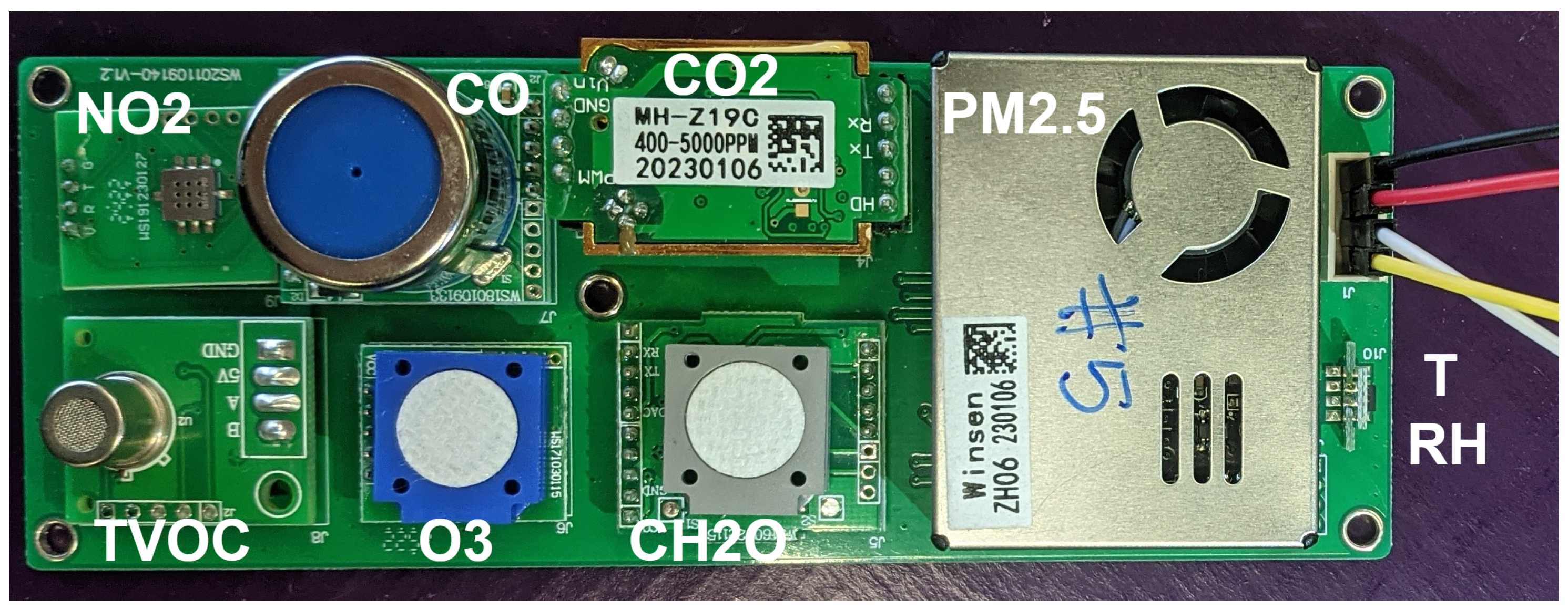
show the daily mean values for each day from 12 to 20 March (the test period) for Node 1 and Node 2, respectively, with details of T and RH in °C and %, respectively; PM1, PM2.5 and PM10 in µg/m³; TVOC in levels; ${\mathrm{CH}}_2$O in mg/m³; and ${\mathrm{CO}}_2$, CO, ${\mathrm{O}}_3$, ${\mathrm{NO}}_2$ in ppm. The sensors and units within the ZPHS01B module are listed in Table 3. In addition,

Table 8. Sensor statistics for both nodes showing minimum (Min), maximum (Max), and standard deviation (Std) values. Units are included in parameter abbreviations.

Parameter	Node 1				Node 2
	Min	Max	Std		Min	Max	Std
PM1 (µg/m3)	11.9	351.9	37.6		14.6	378.8	32.9
PM2.5 (µg/m3)	15.7	453.0	47.4		17.6	492.9	41.8
PM10 (µg/m3)	16.7	611.7	61.8		19.0	653.1	53.4
${\mathrm{O}}_3$ (ppm)	0.02	0.06	0.01		0.02	0.04	0.002
${\mathrm{CH}}_2$O (mg/m3)	0.02	0.13	0.02		0.02	0.08	0.01
${\mathrm{CO}}_2$ (ppm)	402.3	565.5	31.4		401.8	570.5	47.3
CO (ppm)	0.50	0.53	0.003		0.50	0.60	0.008
${\mathrm{NO}}_2$ (ppm)	0.36	10.0	3.46		3.20	10.0	0.97
TVOC (levels)	0.0	3.0	1.05		0.0	3.0	0.68
T (°C)	8.1	20.5	2.7		3.2	24.4	4.0
RH (%)	53.8	99.5	11.5		47.8	113.3	15.4

show the minimum (min.), maximum (max.) and standard deviation (std.) of the readings from these nodes for each day, during this period.

From these tables, in particular Table 6 and Table 7, we see a similar behavior among the sensors from Node 1 and 2, with slight differences due to the small gap in the placement. We must stress that the RH sensor in Node 2 has an offset, with readings above 100%, in particular 113.326%. Notice that, checking Table 8, this Node 2 has RH mean values on days 18th, 19th and 20th higher than 100%. With regard to PM, it can be observed that Node 2 is more affected by fireworks, firecrackers and fumes on the 18th and 19th since it is closer to them. However, when the monument is burned (late at night on the 19th), Node 1 detects higher PM levels due to its proximity to it. Also, we see that TVOCs are higher in Node 1 than in Node 2, in particular on the 15th and 16th, due to the materials used (paints, varnishes and glues) when setting up the monuments. On the other hand, we observe that the CO sensors do not seem to respond (remaining around 0.5 ppm), while the ${\mathrm{NO}}_2$ sensors appear to be saturated, measuring close to the maximum of 10 ppm, particularly Node 2. Notice about the ${\mathrm{NO}}_2$ sensor, as mentioned in Section 3.1.2, this sensor is one of the most sensitive ones and suffers from high cross-sensitivity issues with other gases, this being one of the main reasons for this saturation behavior most of the time.

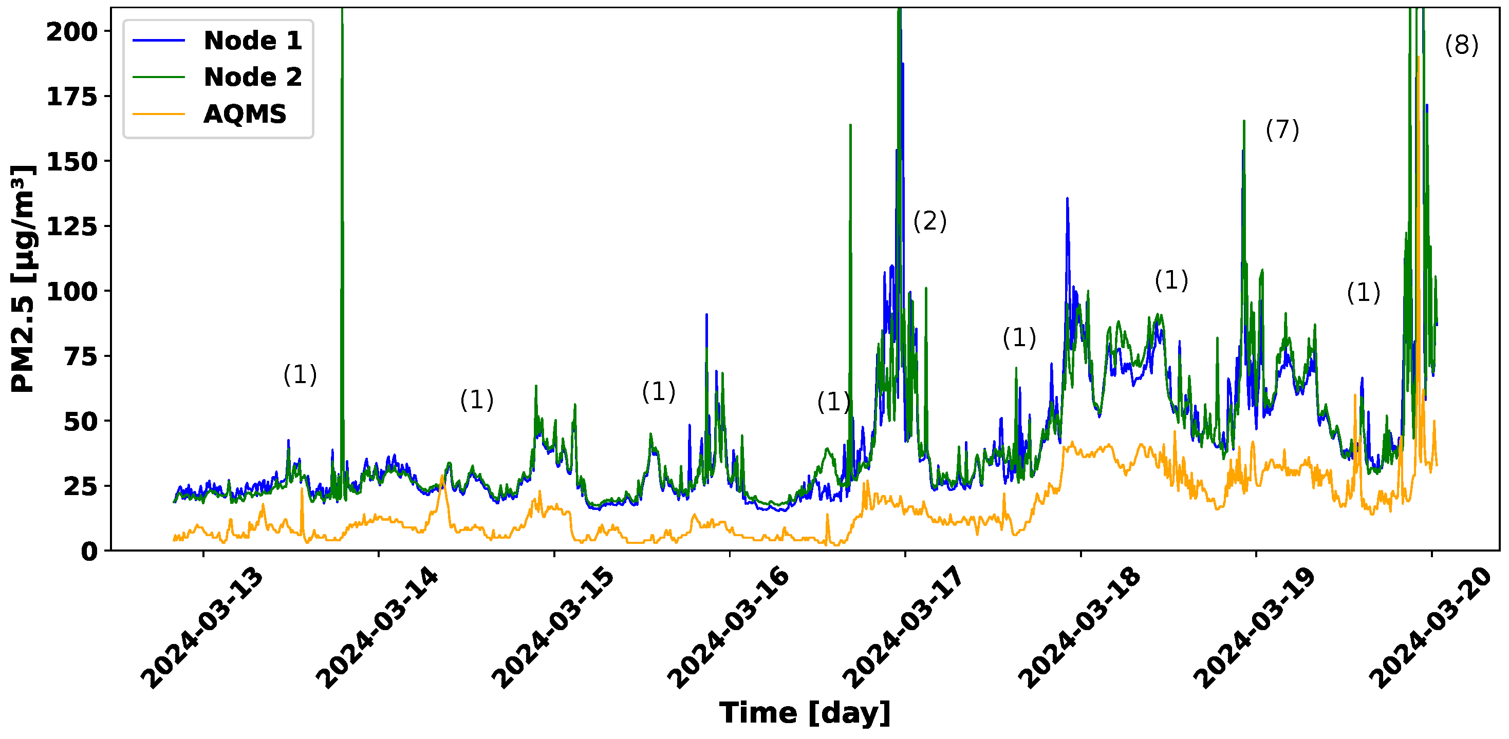
In Figure 9, Figure 10, Figure 11 and Figure 12 are shown the instantaneous readings from Node 1, Node 2 and the AQMS (as a reference) during the test period, for PM2.5, ${\mathrm{O}}_3$, ${\mathrm{NO}}_2$ and CO pollutants, respectively, since they are available both in the AQ IoT nodes and the AQMS. In order to keep the same units, we have translated, according to [39], the readings from Node 1 and 2 into µg/m³, except for CO in mg/m³.

From these figures, we highlight, in Figure 9, how PM increases from March 17th with the maximum on the night of the 19th (denoted as (8) in Table 4). Also, we can see periodically peaks associated with the daily events held at 14:00 everyday, denoted as (1), as well as the events denoted as (2) and (7). Note that these peaks are less defined in the AQMS, as the station is not located in the exact same place and is in a clearer environment, as detailed in Section 3.4. To maintain a better scale and more clearly observe this behavior in Figure 9, we have trimmed the peaks detected in the nodes.

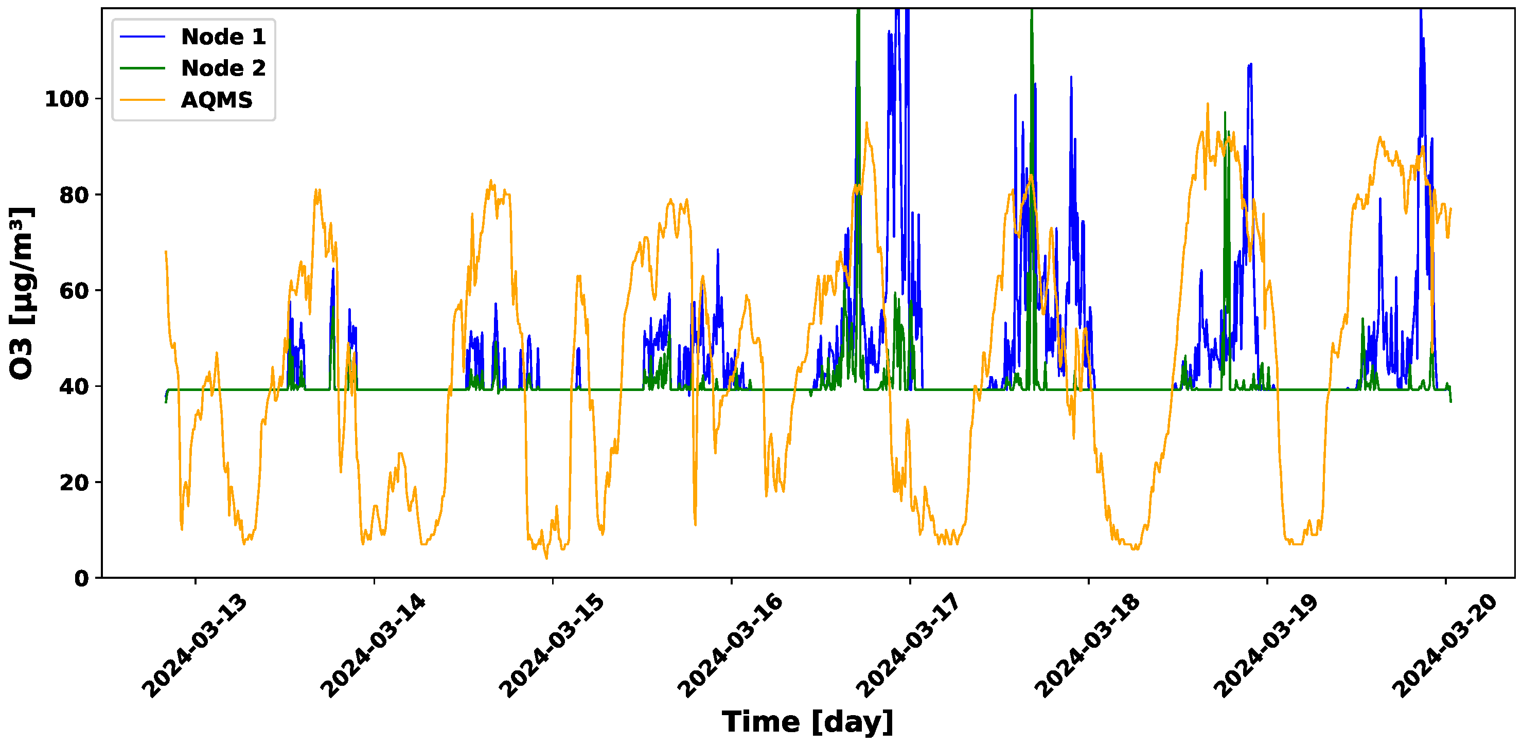
Regarding ${\mathrm{O}}_3$ in Figure 10, we observe a similar pattern and the same tendencies as the AQMS, and both nodes detected a pattern associated with the ${\mathrm{O}}_3$ formation cycle. This gas is generated by complex photochemical reactions involving NO, ${\mathrm{NO}}_2$ and ${\mathrm{SO}}_2$ in the presence of sunlight [40]. It is worth mentioning that the ${\mathrm{O}}_3$ sensor on the ZPHS01B has a minimum detection limit of 0.02 ppm, which corresponds to approximately 40 µg/m³. However, the minimum value recorded by the regulated AQMS is 4 µg/m³. Therefore, this low-cost ${\mathrm{O}}_3$ sensor does not have sufficient resolution to detect ${\mathrm{O}}_3$ concentrations below this threshold.

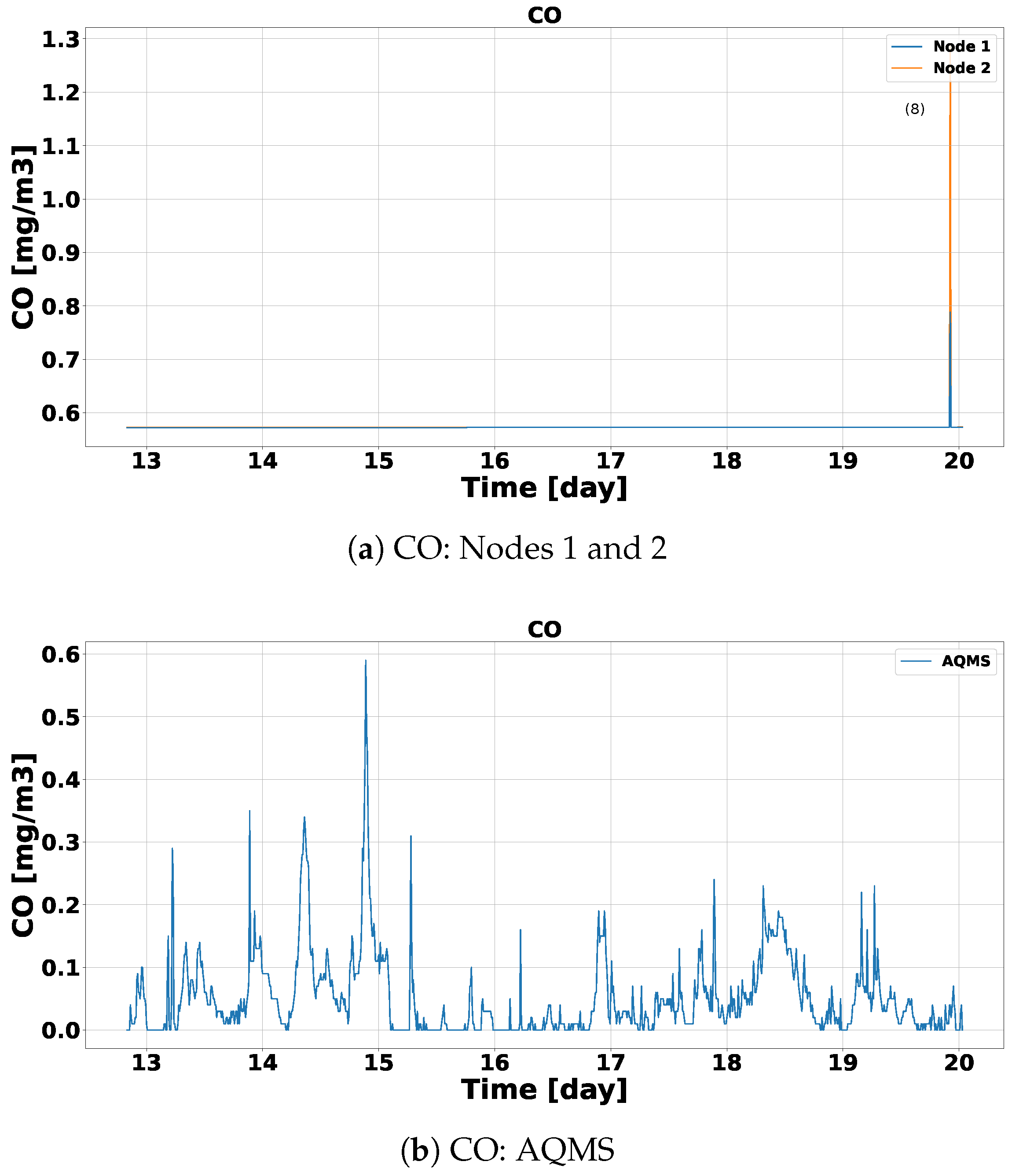
Regarding the ${\mathrm{NO}}_2$ and CO sensors, we observe the same behavior of reduced activation as mentioned earlier. However, we must stress that the CO sensors in Figure 12 show a peak at the end of the festival, that it is related to the main event La Cremà (denoted as (8) in Table 4), when all the monuments are burnt.

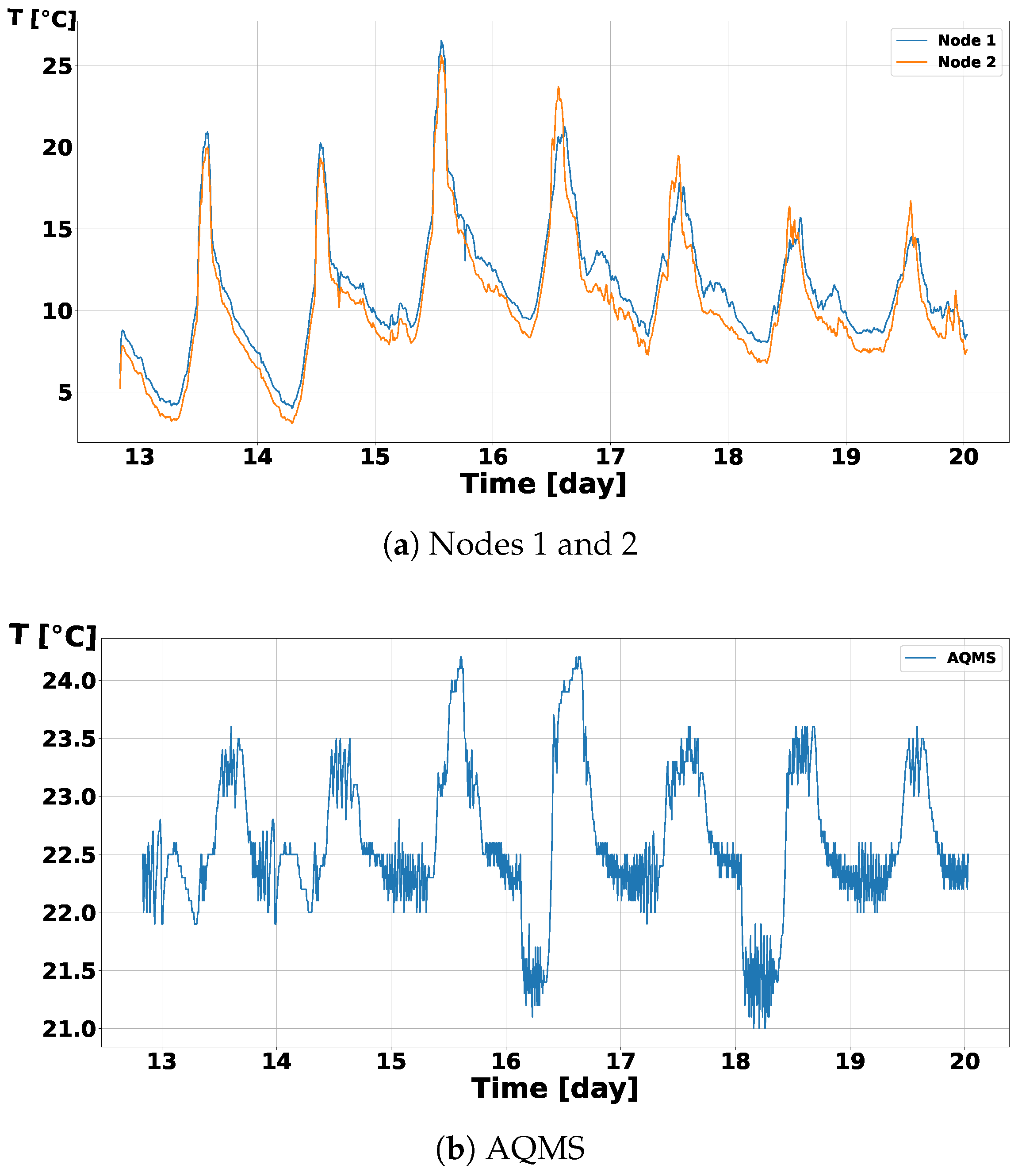
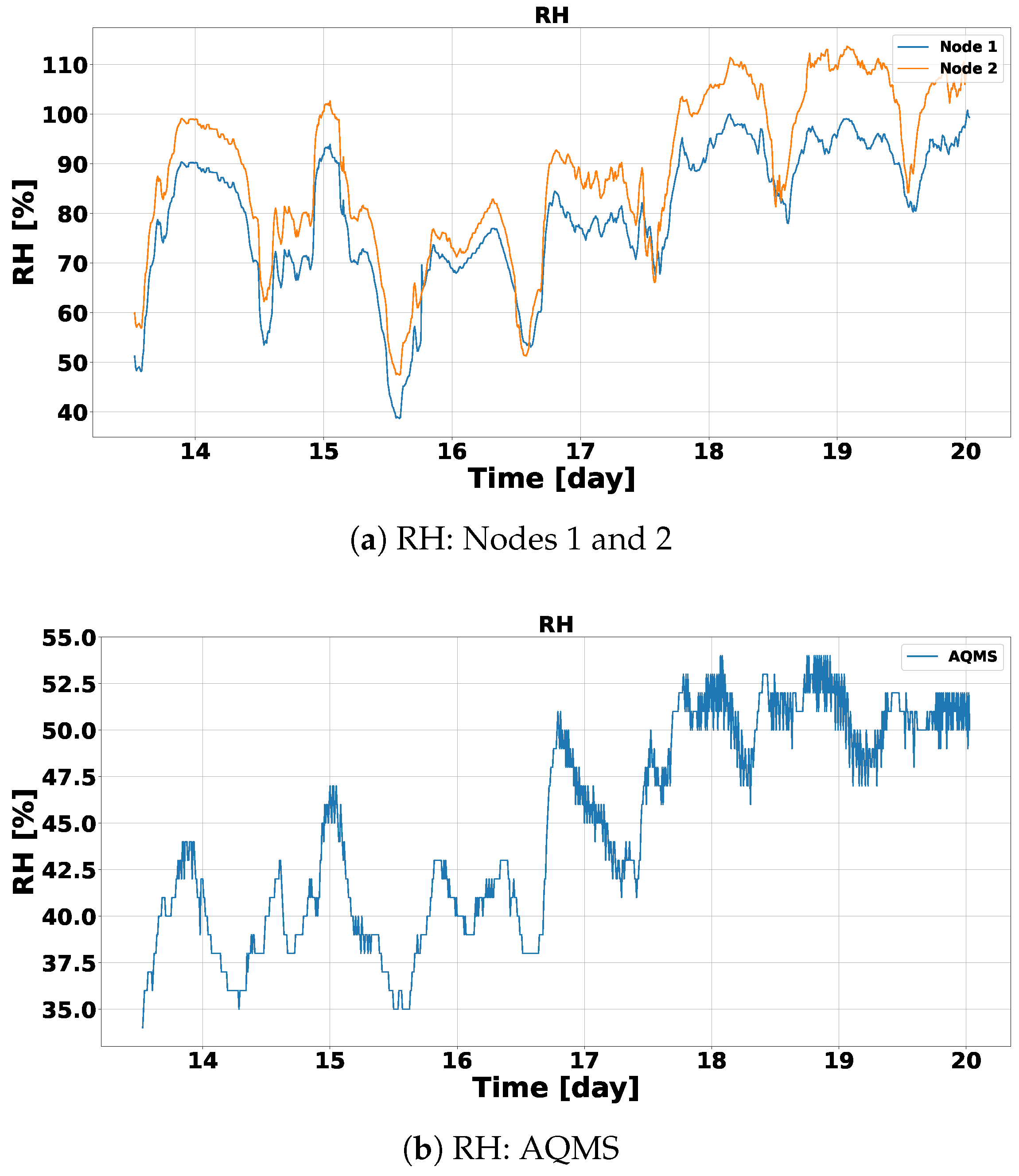
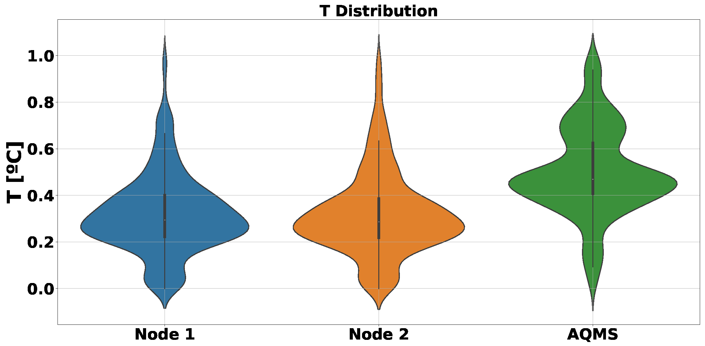
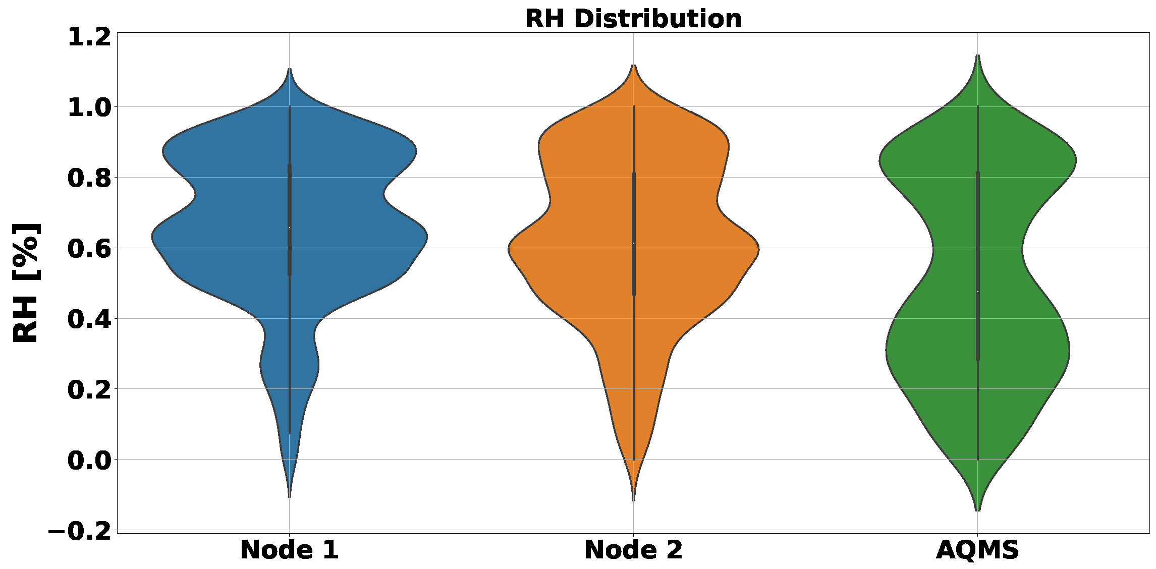
In addition, although not considered as AQ parameters, both T and RH indirectly impact on AQ measurements. Figure 13 and Figure 14 present the instantaneous readings from Node 1, Node 2 and the AQMS during the festival for T and RH, respectively, with virtually the same behavior although, in Node 2 for RH, an offset is clearly observed making readings higher than 100%. Also notice that the AQMS measures T in the station (inside), while the nodes are placed outdoors, showing a lower T.

Further analysis of all these measurements is shown in Figure 15, Figure 16, Figure 17, Figure 18, Figure 19 and Figure 20, which present the violin plots of the normalized measurement distributions during the test period for the T, RH, PM2.5, ${\mathrm{O}}_3$, ${\mathrm{NO}}_2$ and CO sensors, respectively, from Node 1 and Node 2 compared to the AQMS. We normalize their values in order to highlight better their distribution. The similarities between the two nodes are evident, as well as a different scale compared to the AQMS, or reference. However, we can identify a similar histogram shape and behavior, with the same tendencies as the reference. In the case of T and RH, it shows a similar pattern to the bimodal histogram for the day/night cycle. Similarly, PM2.5 and ${\mathrm{O}}_3$ follow a similar shape distribution but at a different scale. Regarding the ${\mathrm{NO}}_2$ and CO sensors, based on the previous results, we cannot confirm clear details.

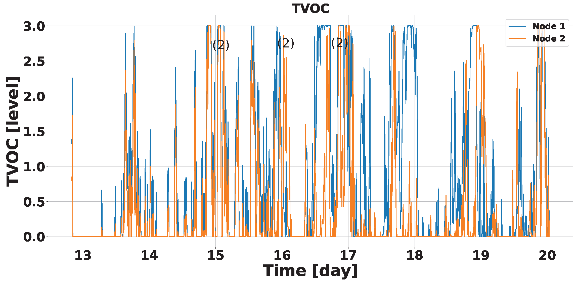
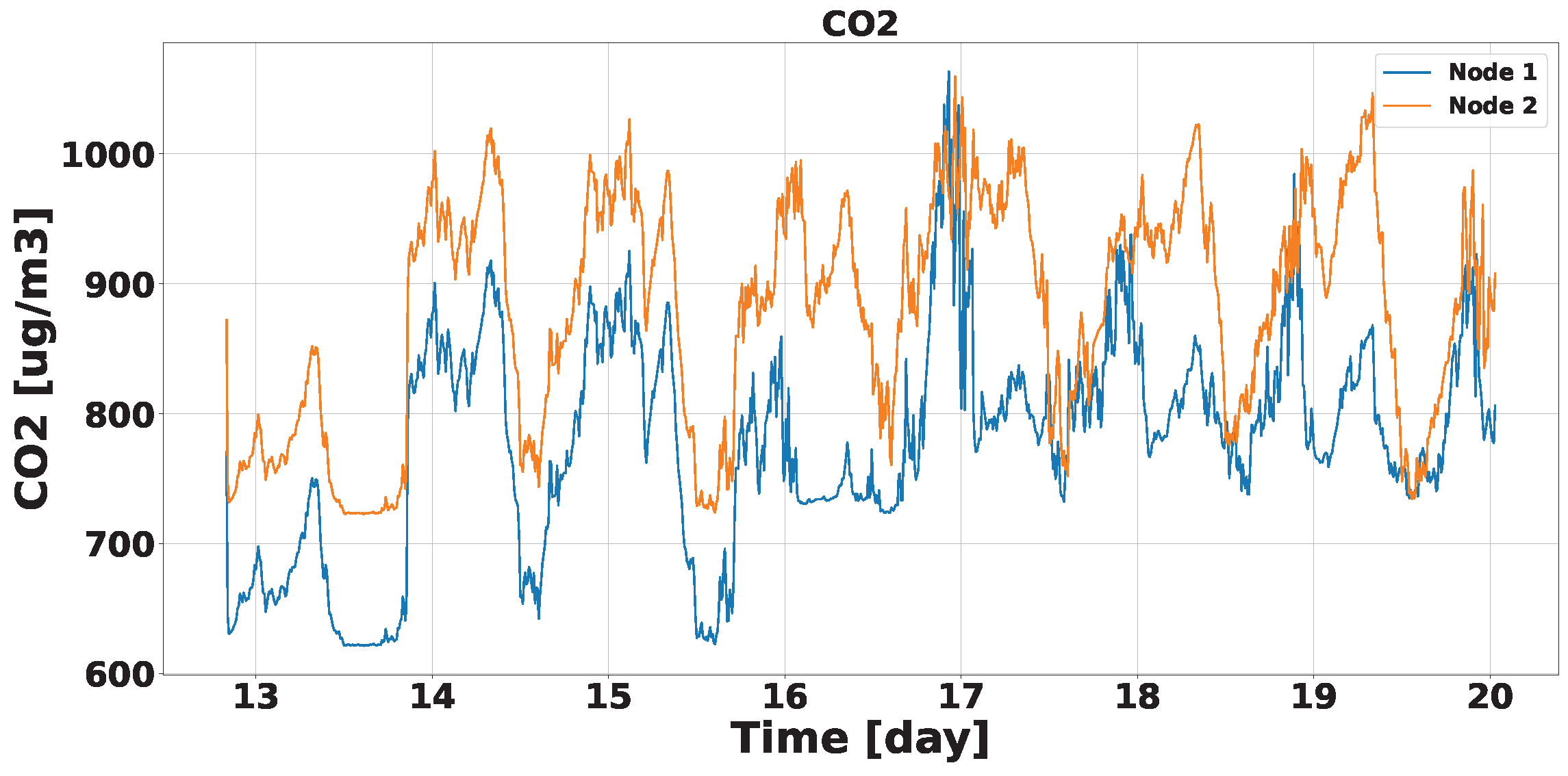
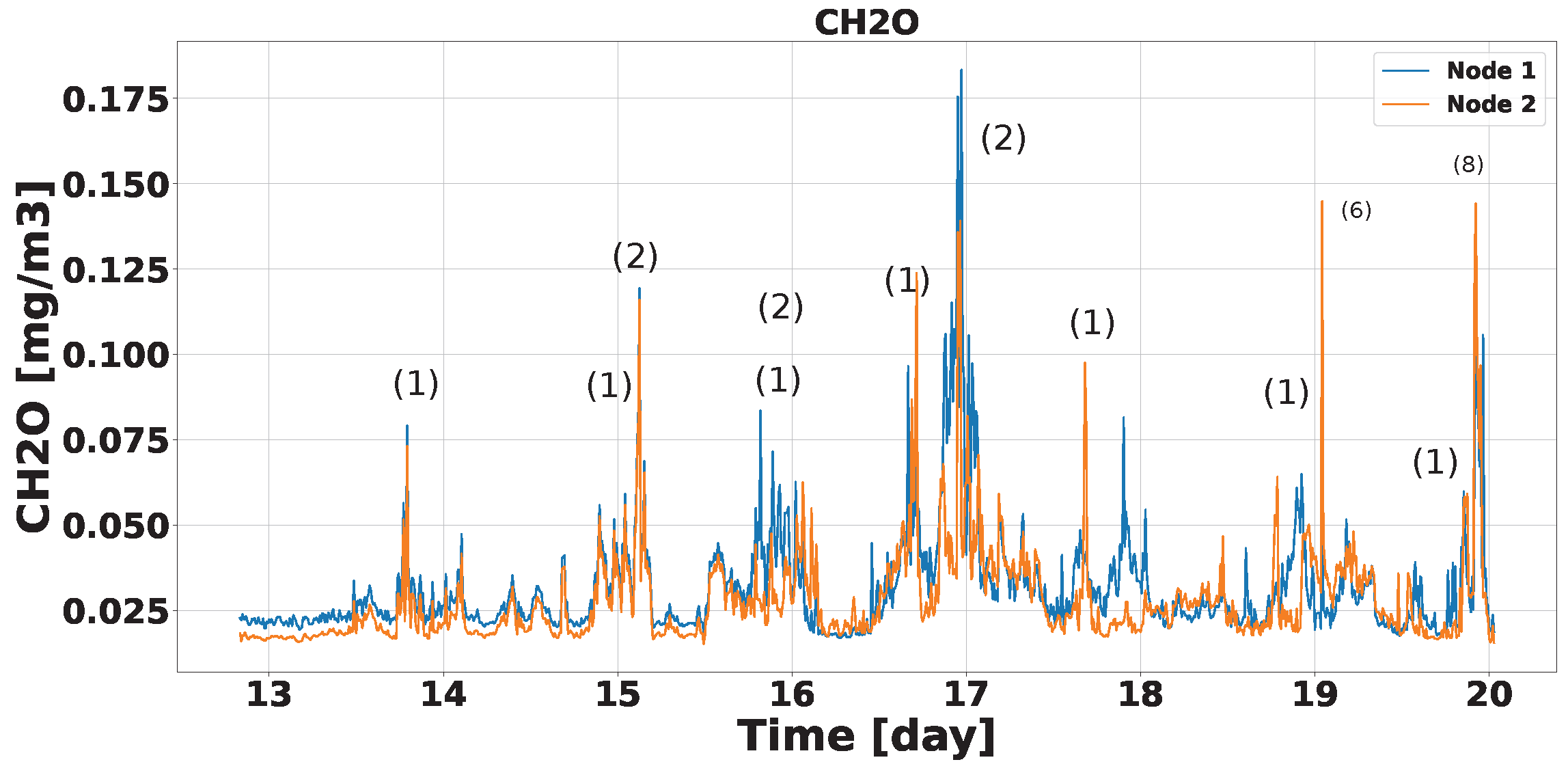
Finally, Figure 21, Figure 22 and Figure 23 show instantaneous readings from pollutants available in the ZPHS01B module (Node 1 and 2), but not available in the AQMS, during the test period, such as TVOCs, ${\mathrm{CO}}_2$ and ${\mathrm{CH}}_2$O. In particular, with regard to TVOCs, higher values are seen between the 15th and 17th due to the monument setup, using paints, varnishes and glues, denoting these events as (2) according to Table 4. Since this sensor only provides four levels, the resolution is low as well as there is high variability between the nodes due to the sensor’s sensitivity, with specific conditions on each node influencing the measurements. The effect of the monument setup (denoted as (2)) can be seen too in the ${\mathrm{CH}}_2$O sensor, Figure 23, that monitors formaldehyde found in the mentioned materials as well as in pyrotechnic products (denoted as (1)), fireworks (denoted as (6) and (8)), fumes and road traffic. Finally, in Figure 22, ${\mathrm{CO}}_2$ shows the human activity and road traffic every day. Notice that these sensors (TVOC, ${\mathrm{CO}}_2$ and ${\mathrm{CH}}_2$O) from Node 1 and 2 behave similarly but with different offsets, in particular for ${\mathrm{CO}}_2$.

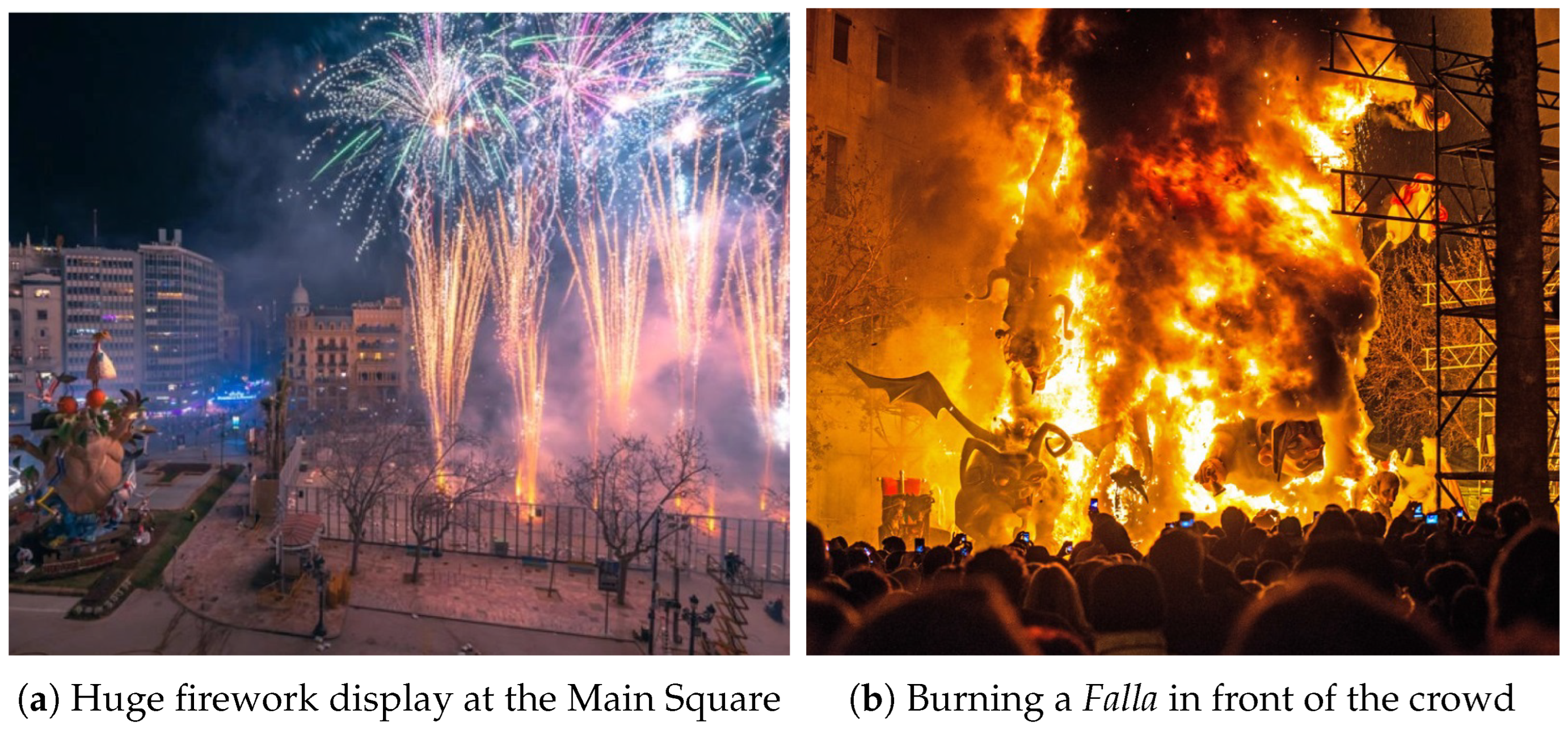
From these previous results, it is clear that this festival alters the AQ, especially in terms of PM. We observe that PM2.5 is the pollutant most directly impacted by fireworks and firecrackers due to the smoke and residual particles they produce.

Also notice that during the first days of the festival (at the beginning), the PM readings are lower as observed in Table 6 and Table 7. However, from March 14th onward, the levels increase until they reach the highest point on the final days. This increase is due to the growing number and intensity of pyrotechnic events, fireworks, fumes and road traffic in general.

Additionally, if we look at Table 4, every day, there are pyrotechnic events scheduled at 14:00 h and 00:00 h. The level of the pollutant reaches the highest peak on 19 March, the day of burning all the monuments (named La Cremà), from 20:00 h till 02:00 am (on the next day), specifically, when the Falla Na Jordana is burnt, where the AQ IoT nodes are placed. Also, we can observe peaks that are associated to explosions of firecrackers launched next to Node 2 as well as more activity in the evenings. Node 1 is closer to the monument and, there, it is not permitted to light firecrackers since it is more crowded.

4.2.2. Calibrated Measurements

From these previous results, we observe that the most accurate sensors, compared to the regulated AQMS and included in the AQG (shown in Table 1), are PM2.5 and ${\mathrm{O}}_3$. Thus, now we perform a calibration analysis on these sensors. Note that PM1 and PM10 are derived from PM2.5, ${\mathrm{NO}}_2$ is saturated and CO is not excited most of the time.

The calibration process is scheduled and performed automatically every 24 h, since the nodes download the ten-minute values from the regulated AQMS everyday. Based on this information, the AQ IoT monitoring nodes adjust the calibration for the next 24 h. For this purpose, each module adjusts the regression models for these calibrated sensors.

We analyze the regression models with different window sizes for the fit, both linear and quadratic. In particular, we compare different window sizes of 1, 4, 8, 12 and 24 h, and present the results of these fits analyzing Root Mean Square Error (RMSE), Mean Absolute Error (MAE) and $R^2$ as performance metrics.

Table 9. Performance metrics for the calibration with PM2.5 for different window sizes: 1, 4, 8, 12 and 24 h.

Window	Node	RMSE	MAE	R2
24	1	7.46	5.35	0.85
	2	7.85	5.36	0.84
12	1	12.46	7.97	0.73
	2	15.54	8.54	0.71
8	1	12.28	7.18	0.68
	2	10.55	7.54	0.66
4	1	14.35	9.44	0.62
	2	24.78	9.24	0.52
1	1	15.75	7.86	0.59
	2	25.12	9.90	0.53

shows the performance metrics for the calibration with PM2.5 for each window size: 1, 4, 8, 12 and 24 h. In this case, we observe that, with a window size of 24 h and a linear regression (i.e., a quadratic regression performs worse), we obtain the best $R^2$ results both in Node 1 and 2. Similarly, in

Table 10. Performance metrics for the calibration with ${\mathrm{O}}_3$ for different window sizes: 1, 4, 8, 12 and 24 h.

Window	Node	RMSE	MAE	R2
24	1	26.35	21.42	0.78
	2	26.96	22.18	0.77
12	1	66.96	39.64	0.66
	2	53.43	38.40	0.64
8	1	46.71	35.97	0.61
	2	47.59	35.86	0,59
4	1	37.08	25.60	0.54
	2	37.15	24.94	0.52
1	1	22.97	12.67	0.50
	2	27.80	14.00	0.49

, we also show these metrics for the calibration of ${\mathrm{O}}_3$, with the same optimal values in window size and regression type. Notice that these nodes (Node 1 and 2) obtain different calibration results and accuracy, due to their low-cost manufacturing process.

As mentioned before, the range of the ${\mathrm{O}}_3$ sensor on the ZPHS01B is shorter than the regulated AQMS and unable to detect values lower than 40 µg/m³. Therefore, this sensor provides worse results compared to the PM2.5 sensor.

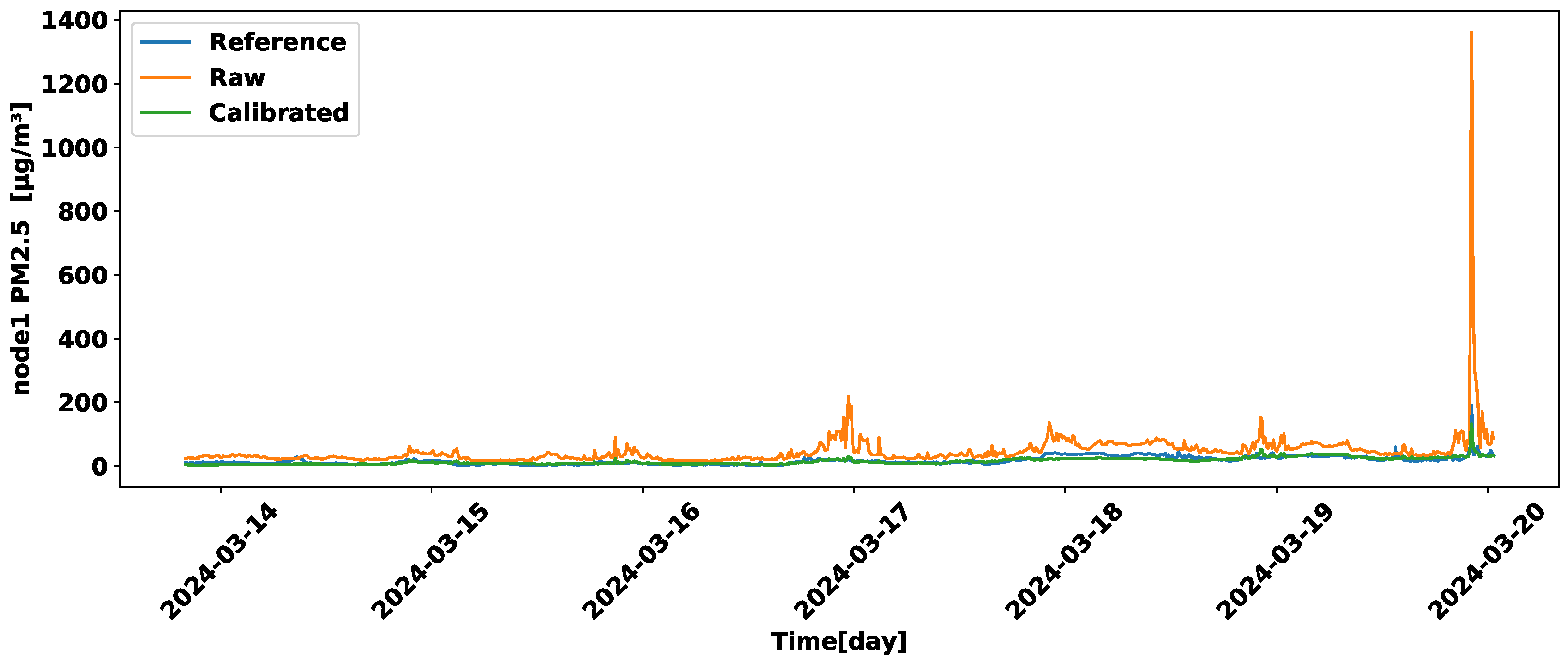
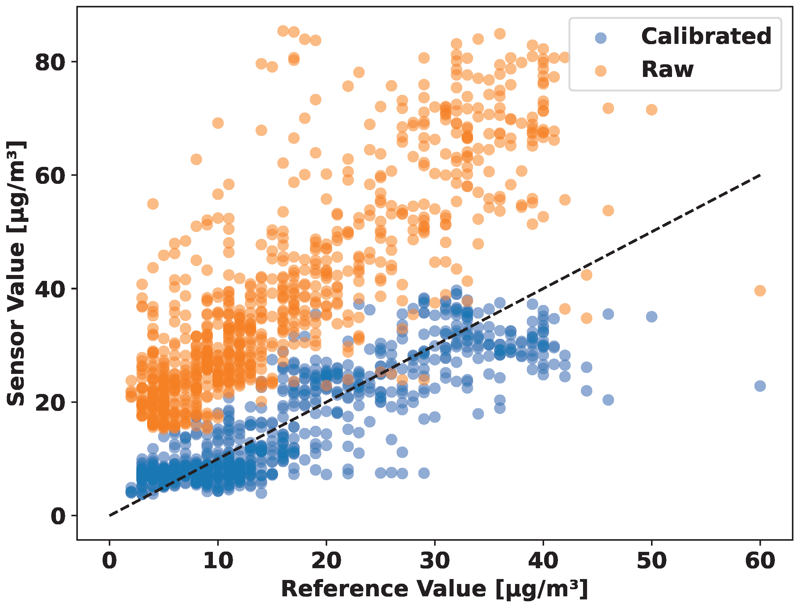
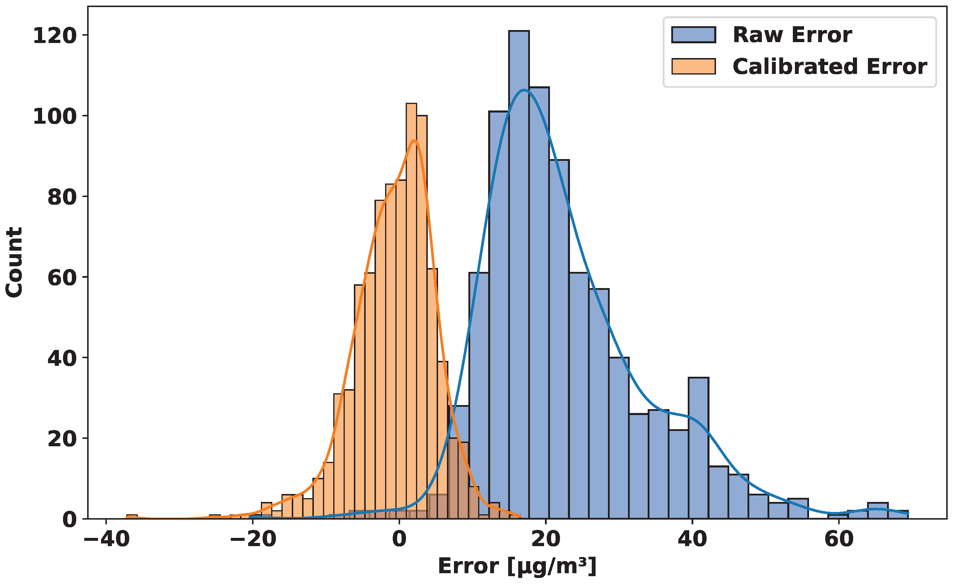
As examples of this calibration process, Figure 24 shows the evolution in time for the calibration results during the experiment for Node 1 with PM2.5 and window size of 24 h, in µg/m³, comparing to the raw and reference AQMS. For this node and sensor, Figure 25 and Figure 26 also show the regression scatter plot and error distribution before and after the calibration process, respectively.

In summary, we propose a low-cost AQ monitoring node that performs calibration automatically every 24 h, in particular for PM2.5 and ${\mathrm{O}}_3$ sensors achieving a coefficient of determination ($R^2$) higher than 0.8. If we compare the proposed node with the related work shown in Section 2, in particular [24,25,26,27], we can observe that this proposal contributes to a more dynamic, efficient and reliable calibration system, easily adapted to LCS features (aging and degradation) and, in addition, it integrates up to nine different sensors, while the rest of the proposals focus on one or two sensors.

5. Conclusions

AQ is measured mainly in terms of PM, ground-level ozone (${\mathrm{O}}_3$), nitrogen oxides (NOx), sulfur dioxide (${\mathrm{SO}}_2$) and carbon monoxide (CO). In urban areas and cities, these pollutants can be extremely hazardous above certain concentrations and should be observed with more detail and resolution, where Low-Cost Sensors (LCSs) play a crucial role.

Many AQ LCSs are available on the market, assembled in boards, modules or systems, but suffer from instability, limited accuracy and cross-sensitivity issues. Among the available alternatives, the ZPHS01B multisensor module offers the highest number of sensors, a good price-to-sensor ratio and a favorable quality-to-price ratio compared to other options. This module measures T, RH, PM1, PM2.5, PM10, CO, ${\mathrm{CO}}_2$, ${\mathrm{NO}}_2$, ${\mathrm{O}}_3$, formaldehyde (${\mathrm{CH}}_2$O) and TVOCs covering all the pollutants within the AQ standards, except ${\mathrm{SO}}_2$. However, our review of related work revealed a lack of information on real-world deployments and their specific details of this module.

In this paper, we provide practical information and recommendations for AQ, including the integration of the off-the-shelf ZPHS01B multisensor module into an AQ IoT node. We conduct a power consumption analysis of this node to optimize energy use through an ON/OFF duty cycle, suggesting 1 min ON and 9 min OFF as a trade-off between power consumption and AQ monitoring standards, taking into account the sensor’s reading stability.

Furthermore, we have assessed the performance of the ZPHS01B multisensor module and all its sensors in a case study where AQ is affected by human activity during Las Fallas in Valencia city, Spain. In this scenario, we have first analyzed the sensors’ performance using raw readings (uncalibrated measurements) to observe the module’s direct outputs. Based on a comparison with the regulated AQMS, we select the sensors with better accuracy for a calibration process, in particular the PM2.5 and ${\mathrm{O}}_3$ sensors.

We found that these sensors, PM and ground-level ozone (${\mathrm{O}}_3$) sensors, provide accurate measurements (compared to the AQMS) with $R^2$ values around 0.8 after calibration using linear regression with a window size of 24 h. Notice that the PM sensor has better range and resolution than the ${\mathrm{O}}_3$ one. The other sensors embedded in the ZPHS01B multisensor module also detected pollutant patterns and trends, but with significantly lower accuracy. Additionally, we observed significant cross-sensitivity issues with the ${\mathrm{NO}}_2$ sensor and high variability between nodes, particularly in the TVOC sensor.

We conclude that this AQ IoT node can serve as a promising starting point for a coarse AQ monitoring solution and for detecting highly polluted areas by enhancing AQ resolution in a cost-effective and straightforward manner. Also notice that, with these nodes, we were able to track the different events held during this festival based on the AQ monitoring.

Our future work involves adjusting and calibrating this module, as shown in [41], since its sensors exhibit the same tendencies as the regulated AQMS. This will allow us to fully exploit its potential. In this context, AI techniques can be particularly useful, as they help address cross-sensitivity issues in the embedded AQ LCS.