An Explicit Transient Rotor Angle Stability Criterion Involving the Fault Location Factor of Doubly Fed Induction Generator Integrated Power Systems

Abstract

Current transient stability analysis of power systems with doubly fed induction generators (DFIGs) draws upon the assumption that nodal electromagnetic power equals to zero during the fault period. The omission of electromagnetic power degrades the fidelity of transient stability analysis and renders the analytical impact of fault location on stability indiscernible. To address this limitation, a DFIG-integrated power system-oriented transient stability mechanism analysis method is proposed involving fault location factors. Firstly, a foundational analysis model is established by integrating a simplified DFIG representation with the improved DC power flow corrected by the fault’s instantaneous short-circuit voltage. Secondly, the non-metallic symmetrical short-circuit fault is equivalently treated as a power injection source, and the faulted electromagnetic power of generators is derived. The proposed equivalence is roughly correct, as its faulted energy integral is validated to approximate ground-truth. Lastly, combining the above analytical formulas and extended equal area criterion (EEAC), a time-domain simulation-free explicit transient stability criterion incorporating fault location factor is settled. Simulation results in a double-generator system with DFIG integration confirm that, compared to existing transient stability criterion, the proposed criterion can expand the stability assessable area by approximately 10% while maintaining accuracy.

1. Introduction

In recent years, wind power penetration has been steadily increasing [1]. A large number of doubly fed induction generators (DFIGs), which operate with electromechanical decoupling characteristics [2], have been integrated into the grid. DFIGs introduce distinct transient stability characteristics from the conventional synchronous generators, which leads to significant changes in the stability modes of power systems with high wind power penetration [3]. Therefore, a comprehensive understanding of the underlying stability mechanisms is urgently required [4].

Transient stability analysis methods for power systems with DFIG integration can be typically classified into two main approaches: time-domain simulation and theoretical analysis. The time-domain simulation approach derives qualitative stability conclusions by comparing transient trajectories under various boundary conditions [5,6,7]. For instance, ref. [5] employed simulation analysis to qualitatively assess the effects of wind power penetration, DFIG parameters and the power system strength on transient stability. Yet, due to the need for repeated tuning of the concerned factors and time-intensive simulations, this method is of limited applicability. Ref. [6] analyzed the transient response characteristics of DFIGs through simulations and found that DFIGs behave as nonlinear power injection sources during faults, affecting system stability through transient power output. Thus, a key challenge arises in the simplification of DFIG’s nonlinearity without introducing substantial errors in faulted power or energy integral, especially when analyzing the transient angle stability boundary. Ref. [7] found that transient characteristics of DFIGs can cause their ability to absorb reactive power after fault clearance, which may weaken the system’s transient stability. However, the time-domain simulation approach yields only qualitative and non-analytical insights and is unable to precisely navigate security dispatch. The requirement to repeatedly solve large-scale differential-algebraic equations (DAEs) via a time-domain simulation (TDS) significantly increases computational complexity and hinders the trustworthiness of quantitative conclusions. The theoretical analysis family is used precisely for this end. It can be further broadly categorized into the energy-based method [8,9], and the explicit criterion-based method [10,11,12]. The former is more suited for analyzing post-fault stability and designing nonlinear controllers, which demand post-fault trajectories collected from phasor measurement units as necessary information. For instance, in terms of a close-loop performance in DFIG-integrated transient stability control, ref. [8] provided a global energy function candidate using post-fault trajectories, and it designed a reinforcement learning-based nonlinear optimal controller to supplement the damping of the excitation system and enhance local active and reactive power control of DFIG. Ref. [9] established a transient model of DFIG with a low voltage ride-through. Based on this model, a Lyapunov energy function was constructed. It was then employed to investigate the impact of voltage and grid strength on energy margin. Yet, in the case of the operating mode formulation or pre-fault preventive control tasks, the energy function method is usually too conservative and ill-suited for such a task, informed with only steady-state equilibrium points. Thus, an explicit criterion-based method arises. Ref. [10] assumed DFIG as a constant power injection source pre-fault and post-clearance while neglecting synchronous machine electromagnetic power during the fault. Through DC power flow analysis, it derived the rotor angle expression and variations in accelerating and decelerating power induced by wind integration. The EEAC was then employed to establish an explicit transient stability criterion. As a follow-up study, ref. [11] investigated the effects of DFIG connected locations and wind power penetration rates on transient stability. Ref. [12] extended the above technical pathways to multi-wind farm integrated grid and found that the change in transient stability is determined by the wind turbine positioned at the outermost boundary of the system. As discussed by many researchers, formulating transient stability criteria from a pre-fault steady-state equilibrium entails explicitly analyzing complex nonlinear, nonconvex, and implicit mappings in DAE systems [13]. This inherently necessitates simplifying assumptions. The assumption in previous studies that synchronous machine electromagnetic power is zero during faults is clearly unrealistic [14]. This also leads to the omission of fault location information. Given that numerous steady-state operating factors affect transient stability [15,16], overlooking any of them may severely compromise precision of stability criteria. A more comprehensive consideration of stability-affecting factors enhances the accuracy of transient stability analysis conclusions. However, this also increases the difficulty of analyzing stability mechanisms.

To conquer these challenges, using the framework proposed in ref. [10,11,12], this paper proposed a new fault location factor-involved transient stability analysis method by incorporating a fault-equivalent power injection source, and a fault instantaneous short-circuit voltage-corrected DC power flow. The changes in acceleration and deceleration areas under different fault locations with DFIG integration are analyzed, and the EEAC is applied to reveal that, under certain conditions, the critical weak point of the power system shifts from the generator to the wind power connection point with DFIG integration.

The structure of this paper is organized as follows: First, Section 2 describes the methodological framework of analysis and fundamental assumptions. Then, Section 3 introduces the derivation of transient stability mechanism. Next, Section 4 details the transient stability analysis considering fault location factors. Section 5 shows the simulation results to verify the effectiveness of the proposed methods. Finally, Section 6 presents the conclusions of this paper.

2. Methodological Framework and Fundamental Assumptions

2.1. Simplified Analytical System

This paper focuses on the first-swing stability mechanism of rotor angles in wind–thermal bundled systems. A large-scale DFIG-based wind farm is equivalently represented by a single DFIG, thereby establishing a representative double-generator system with DFIG integration, as shown in Figure 1.

For the double-generator system, the second-order differential equation of rotor angle is expressed as

$$\left\{\begin{array}{c}{\displaystyle \frac{2H_1}{{\omega }_0}}{\displaystyle \frac{d{\delta }_1^2}{d{t}^2}}=P_{m1}-P_{e1}\\ {\displaystyle \frac{2H_2}{{\omega }_0}}{\displaystyle \frac{d{\delta }_2^2}{d{t}^2}}=P_{m2}-P_{e2}\end{array}\right.,$$

(1)

where H represents the inertia constant of the synchronous generator, ω represents the electrical angle velocity, and δ represents the rotor angle, P_m and P_e represents the mechanical and electromagnetic power, respectively. Subscripts “1” and “2” indicate variables related to the synchronous generators G1 and G2, respectively, while subscript “0” refers to the steady-state variable before the fault occurs.

Then, the motion equation of the one-machine infinite-bus (OMIB) system [12] is written as

$${\displaystyle \frac{2H}{{\omega }_0}}{\displaystyle \frac{d{\delta }^2}{d{t}^2}}=P_m-P_e,$$

(2)

in the formulation:

$$\delta ={\delta }_1-{\delta }_2,$$

(3)

$$H={\displaystyle \frac{H_1{H}_2}{H_1+H_2}},$$

(4)

$$P_m={\displaystyle \frac{H_2}{H_1+H_2}}{P}_{m1}-{\displaystyle \frac{H_1}{H_1+H_2}}{P}_{m2},$$

(5)

$$P_e={\displaystyle \frac{H_2}{H_1+H_2}}{P}_{e1}-{\displaystyle \frac{H_1}{H_1+H_2}}{P}_{e2}.$$

(6)

The impact of DFIG integration on rotor angle variation in the OMIB system can be expressed as follows:

$$\Delta \delta ={\delta }_W-\delta ,$$

(7)

$${\displaystyle \frac{d\Delta {\delta }^2}{d{t}^2}}={\displaystyle \frac{{\omega }_0}{2H_W}}(P_{mW}-P_{eW})-{\displaystyle \frac{{\omega }_0}{2H}}(P_m-P_e),$$

(8)

in the formulation, the subscript “W” denotes variables with the integration of DFIG.

During fault, the difference between the mechanical power and the electromagnetic power of the system represents the acceleration power $P_{acc}$. After fault clearance, this difference corresponds to the deceleration power $P_{dec}$. With the integration of DFIG, the corresponding changes in acceleration power and deceleration power can be expressed as follows:

$$\left\{\begin{array}{c}\Delta P_{acc}=\left|(P_{mW}-P_{eW}^F)\right|-\left|(P_m-P_e^F)\right|\\ \Delta P_{dec}=\left|(P_{mW}-P_{eW}^C)\right|-\left|(P_m-P_e^C)\right|\end{array}\right.,$$

(9)

in the formulation, the superscript “F” represents the fault duration period, while the superscript “C” represents the post-fault clearance period.

According to EEAC, when the fault duration remains unchanged, if the DFIG integration results in a decrease in the acceleration power ($∆P_{acc}<0$) and an increase in the deceleration power ($∆P_{dec}>0$), the transient stability of the system is enhanced [17]. Conversely, if the opposite trend is observed, the transient stability decreases. The specific criteria are summarized in

Table 1. Judgment principle of transient stability.

The Change in Acceleration and Deceleration Power	The Change in Stability
$\Delta P_{acc}>0\&\Delta P_{dec}<0$	Decrease
$\Delta P_{acc}<0\&\Delta P_{dec}>0$	Increase
$\Delta P_{acc}<0\&\Delta P_{dec}<0$$\Delta P_{acc}>0\&\Delta P_{dec}>0$	Uncertain

.

If the variations in the electromagnetic and mechanical power of synchronous generators with DFIG integration can be derived, the impact of DFIG integration on the transient stability can be systematically analyzed. To analytically establish the correlation between operational boundary conditions and stability mechanisms, three assumptions are introduced, as follows:

• The DFIG is equivalent to a power injection model. When the stator voltage drop of the DFIG is not significant during fault, the wind turbine continues to deliver its pre-fault steady-state power output. Thus, the DFIG can be equivalently modeled as a power source throughout the fault duration. Detailed simulation validation can be found in Appendix A.
• The electromagnetic power is calculated through the DC power flow model [10]. The transient stability change trend of the system can be approximately inferred from the variations in power flow distribution.
• When the fault occurs, the electromagnetic power of the synchronous generator is affected by factors such as the wind power connection point, fault duration, and fault location, and is generally non-zero. For the most severe three-phase non-metallic short-circuit fault at the sending end, assuming that the non-periodic components of current and voltage during fault are negligible, the fault can be approximated as an equivalent power source. Under this assumption, the DC power flow model can be employed to estimate the electromagnetic power distribution during the fault period.

The multi-generator system can be equivalently modeled as the simplified double-generator system shown in Figure 1 by employing the method described in Appendix B.1 [18]. Stability analysis can then be performed using the subsequent methods.

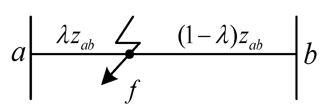
2.2. Derivation of Eequivalent Fault Power Injection Model

During fault, the current and voltage of power systems consist of both periodic components and non-periodic components that decay over time. To simplify the analytical derivation, this paper considers only the periodic components, without addressing the computation of non-periodic components.

It is assumed that a non-metallic short circuit occurs at node f through a transitional resistance $R_g$. From the perspective of the pre-fault network, this condition is equivalent to an additional injection current ${\dot{\mathit{I}}}_{\mathit{f}}$ at the fault node, as shown in Figure 2.

At the fault node f, the system satisfies the following relationship:

$$\dot{{\mathit{V}}_{\mathit{f}}}={\dot{\mathit{V}}}_f^{\left(0\right)}-Z_{ff}\dot{{\mathit{I}}_{\mathit{f}}}.$$

(10)

In the formulation, $\dot{{\mathit{V}}_{\mathit{f}}}$ represents the voltage at node f during fault, while ${\dot{\mathit{V}}}_f^{\left(0\right)}$ corresponds to the pre-fault steady-state voltage at the same node. Z_ff represents the self-impedance at node f, and ${\dot{\mathit{I}}}_{\mathit{f}}$ is the short-circuit current at node f.

Based on the current–voltage relationship, it follows that

$$\dot{{\mathit{V}}_{\mathit{f}}}-R_g\dot{{\mathit{I}}_{\mathit{f}}}=0.$$

(11)

By combining and solving (10) and (11), the following result is obtained:

$$\dot{{\mathit{I}}_{\mathit{f}}}={\dot{\mathit{V}}}_f^{\left(0\right)}/(Z_{ff}+R_g).$$

(12)

The equivalent fault power injected at node f is obtained through calculation as

$$P_f=-{\dot{V}}_f{\dot{I}}_f^{*}=-R_g{\dot{I}}_f{\dot{I}}_f^{*}=-R_g{\left|{\dot{I}}_f\right|}^2=-R_g{\displaystyle \frac{{(V_f^{(0)})}^2}{{\left|Z_{ff}+R_g\right|}^2}},$$

(13)

where $P_f$ is the equivalent fault power injection source.

Equation (13) indicates that the equivalent fault injected power is influenced only by the transitional resistance, the self-impedance at the fault node and the pre-fault voltage at the same node. When a short circuit occurs at any location, the relative distance between the fault node f and node a with respect to the total line is $\lambda$, while the relative distance between node f and b node is $(1-\lambda )$, as shown in Figure 3.

The impedance Z_ff and Z_fc can be calculated through the node impedance matrix. The self-impedance at the fault node f and the mutual impedance between node f and any node c can be obtained from Appendix C, as follows:

$$Z_{ff}={(1-\lambda )}^2{Z}_{aa}+{\lambda }^2{Z}_{bb}+2\lambda (1-\lambda )Z_{ab}+\lambda (1-\lambda )z_{ab},$$

(14)

$$Z_{cf}={\dot{V}}_f={\dot{V}}_a-{\dot{I}}_{aB}\lambda z_{ab}=Z_{ac}-{\displaystyle \frac{Z_{ac}-Z_{bc}}{z_{ab}}}\lambda z_{ab}=(1-\lambda )Z_{ac}+\lambda Z_{bc},$$

(15)

where $Z_{aa},Z_{bb},Z_{ab},Z_{ac},Z_{bc}$ represent the elements of the node impedance matrix corresponding to nodes $a,b,c$. $z_{ab}$ represents the impedance of the transmission line between nodes $a,b$.

When the per-unit values of the normal voltage components at each node are set to 1. Consequently, the actual voltage at any node c after fault is

$$\dot{{\mathit{V}}_{\mathit{c}}}=1-{\displaystyle \frac{Z_{fc}}{Z_{ff}+R_g}}.$$

(16)

3. Derivation of Transient Stability Mechanism

Based on the aforementioned model, the electromagnetic power variation in synchronous generators with and without DFIG integration can be analytically derived via the DC power flow model. Explicit expressions for the mechanical and electromagnetic power of OMIB system during steady-state period, fault period, and post-fault period are obtained. Subsequently, EEAC is employed to evaluate the change in power system transient stability. The detailed steps of the derivation are provided in Appendix B.2.

3.1. Steady-State Period

3.1.1. Without DFIG Integration

According to the DC power flow model, the steady-state rotor angle between two generators satisfies

$${\delta }_0={\delta }_1-{\delta }_2=P_{G1}x-P_L(x-x_L),$$

(17)

where $P_{G1}$ denotes the active power output of G1 at a steady-state and $P_L$ denotes the total load, which is modeled as a constant impedance. x describes the electrical distance between G1 and G2 and $x_L$ is the electrical distance between G1 and the load.

According to the classical second-order model of the synchronous generator, the mechanical power equals its steady-state active power output. Consequently, the mechanical power expression of the OMIB system is derived as follows:

$$P_m={\displaystyle \frac{H_2}{H_1+H_2}}{P}_{m1}-{\displaystyle \frac{H_1}{H_1+H_2}}{P}_{m2}=P_{G1}-{\alpha }_H{P}_L,$$

(18)

in the formulation, the inertia ratio ${\alpha }_H$ is defined as ${\alpha }_H=H_1/(H_1+H_2)$, which means the ratio of the inertia constant of G1 to the total inertia constant of G1 and G2.

3.1.2. With DFIG Integration

With DFIG integration, the steady-state rotor angle changes to

$${\delta }_{0W}=P_{G1}x-P_L(x-x_L)+\gamma P_L(1-k-\beta )x,$$

(19)

where the DFIG connection ratio k is defined as the ratio of the electrical distance from the DFIG connection point to G1, relative to the electrical distance between G1 and G2; $\gamma$ denotes the wind power penetration, defined as $P_W=\gamma P_L$, where $P_W$ is the active power output of DFIG; the imbalance coefficient $\beta$ can be described as

$$\left\{\begin{array}{c}{P}_{G1W}=P_{G1}-\beta \gamma P_L\\ P_{G2W}=P_{G2}-(1-\beta )\gamma P_L\end{array}\right..$$

(20)

Considering that DFIG is directly integrated into the grid, the total load remains unchanged, the inertia of the synchronous generators remains unchanged with and without DFIG integration, and the generators reduce their active output to maintain power balance. The mechanical power expression of the system with DFIG integration is derived as follows:

$$P_{mW}={\displaystyle \frac{H_2}{H_1+H_2}}{P}_{G1W}-{\displaystyle \frac{H_1}{H_1+H_2}}{P}_{G2W}=P_{G1}-\beta \gamma P_L-{\alpha }_H(1-\gamma )P_L.$$

(21)

The change in the steady-state rotor angle of the system with and without the DFIG integration is

$$\Delta {\delta }_0={\delta }_{0W}-{\delta }_0=\gamma P_L(1-k-\beta )x.$$

(22)

3.2. Fault Period

Due to the consideration of the most severe three-phase symmetric fault in this paper, the voltage drops at various nodes in the system during the fault period. This situation conflicts with the assumption that the voltage level is approximately 1 in the DC power flow model, which leads to inaccuracies in calculating electromagnetic power during the fault period with traditional DC power flow models. Thus, to improve the accuracy of calculating the electromagnetic power distribution of synchronous generators during fault, this paper introduces a fault instantaneous short-circuit voltage-corrected DC power flow model and presents the following assumptions:

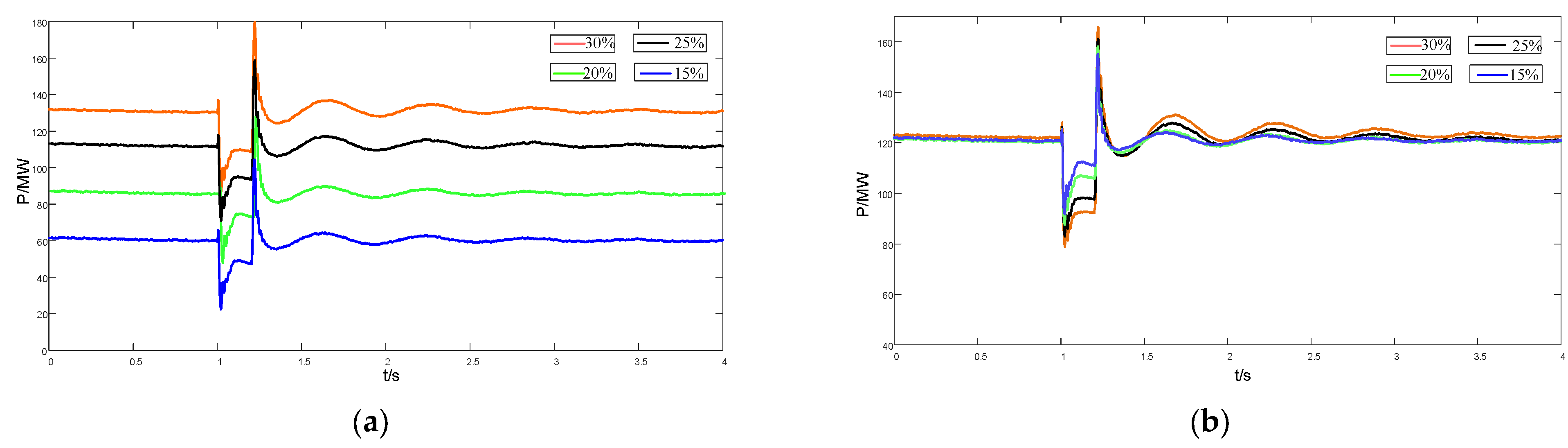
• During fault, the electromagnetic power of DFIG experiences an initial drop, followed by an overshoot after a certain period, ultimately recovering to the level close to the pre-fault power. If a detailed power model is used for modeling, it will inevitably make subsequent transient stability criterion difficult to analyze. Given that the EEAC mainly emphasizes the accumulation of transient energy during faults, the electromagnetic power of DFIG may be approximated by a simplified constant power injection model. As long as the accumulated energy during the fault period is made to align closely with the actual value, significant errors will not be introduced into the EEAC, while the analytical solvability of the transient stability criteria is maintained. Therefore, the electromagnetic power of the DFIG during the fault period can be expressed as

  $$P_W^F=\mu P_W,$$

  (23)

  where $\mu$ is the DFIG output reduction coefficient, which reflects the decrease in DFIG output due to voltage drop during the fault. The value of the coefficient can be approximately calculated from simulation data across various operational modes. It is defined as the integral of the DFIG electromagnetic power during the fault, divided by the fault duration and the steady-state output power. For a more precise estimation of this coefficient, the method presented in ref. [19] can be applied, which uses multiple linear regression with fault location codes and steady-state parameters as inputs. Given the limitations of length and the desire to highlight the main points of this paper, a detailed discussion of this method will not be provided here but will be considered for future research.
• The non-periodic components of the electromagnetic power, voltage, and current of the synchronous generator during the fault period is ignored. According to simulation results, the amplitude of the nominal frequency periodic component of the electromagnetic power of synchronous generators remains relatively stable during the fault, while the non-periodic components diminish rapidly. Thus, when analyzing rotor angle stability during faults, it is sufficient to ignore the non-periodic components and focus solely on the periodic components.
• The non-nominal frequency harmonics of voltage and current of synchronous generators during fault is ignored. Ref. [20] demonstrates that non-nominal frequency harmonics occupy a relatively small proportion and decay rapidly during fault, resulting in minimal effects on power angle stability compared with nominal frequency component. Since this paper investigates transient rotor angle stability, the impact of non-nominal frequency harmonics is overlooked.

Based on the above assumptions and explanations, a fault instantaneous short-circuit voltage-corrected DC power flow model is proposed to match the derivation process during the fault.

During the fault, the voltage amplitude of any node c is

$${\phi }_c=\left|{\dot{V}}_c\right|=\left|1-{\displaystyle \frac{Z_{cf}}{Z_{ff}+R_g}}\right|,$$

(24)

where ${\phi }_c$ is the voltage amplitude of node c, and G1 and G2 are defined as node 1 and 2, the load is node 3, and the fault node is node 4, then there is

$$\phi =[{\phi }_2,{\phi }_2,{\phi }_3,{\phi }_4].$$

(25)

According to the power flow equation of power systems, n indicates all nodes, and the injected power of any node c is

$$P_c=\left|V_c\right|{\displaystyle \sum _{j=1}^n\left|V_j\right|}(G_{cj}\cos {\theta }_{cj}+B_{cj}\sin {\theta }_{cj}).$$

(26)

At the same time, the assumption of the DC power flow model is used by ignoring the resistance of the branch, and the phase angle difference between the two ends of the branch is small, and bringing in the voltage amplitude of each point, we can obtain the following:

$$P_c={\phi }_c{\displaystyle \sum _{j=1}^n{\phi }_c}{B}_{cj}({\theta }_c-{\theta }_c).$$

(27)

This makes it possible to calculate the approximate power distribution during the fault period.

3.2.1. Without DFIG Integration

When the fault location factor is neglected and the electromagnetic power of the synchronous generators is assumed to be approximately zero during fault [10], the differential equation of $∆\delta$ is

$$\left\{\begin{array}{c}(P_{mW}-P_{eW}^F)-(P_m-P_e^F)=({\alpha }_H-\beta )\gamma P_L\\ {\displaystyle \frac{d\Delta {\delta }^2}{d{t}^2}}={\displaystyle \frac{{\omega }_0}{2H}}({\alpha }_H-\beta )\gamma P_L\end{array}\right..$$

(28)

When considering the fault location factor, the electromagnetic power of the OMIB system during fault without DFIG integration, can be approximately expressed as

$$P_e^F={\displaystyle \frac{H_2}{H_1+H_2}}{P}_{e1}^F-{\displaystyle \frac{H_1}{H_1+H_2}}{P}_{e2}^F={\displaystyle \frac{\delta +\frac{{\phi }_3}{{\phi }_2}{P}_L(x-x_L)-P_f\frac{x_f}{{\phi }_3{\phi }_4}}{\frac{x_L}{{\phi }_1{\phi }_4}+\frac{x-x_L}{{\phi }_2{\phi }_3}}}-{\alpha }_H{\phi }_3^2{P}_L,$$

(29)

where $P_f$ is the equivalent fault power injection source without DFIG integration, and $x_f$ represents the electrical distance from the fault location to the load.

By assuming that the per-unit values of the steady-state voltage magnitudes at all nodes are set to 1, (13) can be expressed as

$$P_f=-R_g{\displaystyle \frac{1}{{\left|Z_{ff}+R_g\right|}^2}}.$$

(30)

In the formulation, the transition resistance $R_g$ is a constant, and the self-impedance Z_ff at the fault node is expressed as follows:

$$Z_{ff}=x_f-{\displaystyle \frac{\left(1-i\right)x_f^2}{x_L}}+z_L,$$

(31)

where $z_L$ represents the impedance of the load, and i denotes the imaginary unit. The detailed steps of the derivation of Z_ff are provided in Appendix D.

Following (18) and (29), without DFIG integration, $P_m-P_e^F$ is calculated as follows:

$$P_m-P_e^F=P_{G1}-{\displaystyle \frac{\delta +\frac{{\phi }_3}{{\phi }_2}{P}_L(x-x_L)-P_f\frac{x_f}{{\phi }_3{\phi }_4}}{\frac{x_L}{{\phi }_1{\phi }_4}+\frac{x-x_L}{{\phi }_2{\phi }_3}}}-{\alpha }_H(1-{\phi }_3^2)P_L.$$

(32)

3.2.2. With DFIG Integration

We define the DFIG integration node as node 5, and the voltage amplitude of each node is expressed as follows:

$$\phi =[{\phi }_{1W},{\phi }_{2W},{\phi }_{3W},{\phi }_{4W},{\phi }_{5W}].$$

(33)

With DFIG integration, the electromagnetic power of the OMIB system during the fault becomes

$$P_{eW}^F={\displaystyle \frac{H_2}{H_1+H_2}}{P}_{e1W}^F-{\displaystyle \frac{H_1}{H_1+H_2}}{P}_{e2W}^F={\displaystyle \frac{\delta -\mu P_W(\frac{x_L-kx}{{\phi }_{4W}{\phi }_{5W}}+\frac{x-x_L}{{\phi }_{2W}{\phi }_{3W}})+\frac{{\phi }_{3W}}{{\phi }_{2W}}{P}_L(x-x_L)-P_{fW}\frac{x_f}{{\phi }_{3W}{\phi }_{4W}}}{\frac{kx}{{\phi }_{1W}{\phi }_{5W}}+\frac{x_L-kx}{{\phi }_{4W}{\phi }_{5W}}+\frac{x-x_L}{{\phi }_{2W}{\phi }_{3W}}}}-{\alpha }_H({\phi }_{3W}^2-\gamma )P_L.$$

(34)

Since the expression of the equivalent electromagnetic power is too complex, and for the sake of simplification in the future, it is worth remembering the following:

$$hx={\displaystyle \frac{kx}{{\phi }_{1W}{\phi }_{5W}}}+{\displaystyle \frac{x_L-kx}{{\phi }_{4W}{\phi }_{5W}}}+{\displaystyle \frac{x-x_L}{{\phi }_{2W}{\phi }_{3W}}},$$

(35)

where h is the structural parameter of the system, which can be calculated according to the impedance distribution of the system. Then, the electromagnetic power expression can be reduced to

$$P_{eW}^F={\displaystyle \frac{\delta }{hx}}-P_W(\mu -{\displaystyle \frac{\mu k}{{\phi }_{1W}{\phi }_{5W}h}})+P_L{\displaystyle \frac{{\phi }_{3W}(x-x_L)}{{\phi }_{2W}hx}}-P_{fW}{\displaystyle \frac{x_f}{{\phi }_{3W}{\phi }_{4W}hx}}-{\alpha }_H({\phi }_{3W}^2-\gamma )P_L.$$

(36)

The self-impedance Z_ffW at the fault node with DFIG integration is expressed as follows:

$$Z_{ffW}=x_f+{\displaystyle \frac{\left(1-i\right)x_f^2}{kx-x_L}}+z_L.$$

(37)

Following (21) and (36), with DFIG integration, $P_{mW}-P_{eW}^F$ is calculated as follows:

$$P_{mW}-P_{eW}^F=P_{G1}-{\displaystyle \frac{\delta }{hx}}-P_L{\displaystyle \frac{{\phi }_{3W}(x-x_L)}{{\phi }_{2W}hx}}+(\mu -{\displaystyle \frac{\mu k}{{\phi }_{1W}{\phi }_{5W}h}}-\beta )P_W+P_{fW}{\displaystyle \frac{x_f}{{\phi }_{3W}{\phi }_{4W}hx}}-{\alpha }_H(1-{\phi }_{3W}^2)P_L.$$

(38)

Considering that there is no significant effect on the voltage amplitude during the fault with the DFIG integration, i.e., ${\phi }_c\approx {\phi }_{cW}$. In the meantime

$${\displaystyle \frac{x_L}{{\phi }_1{\phi }_4}}+{\displaystyle \frac{x-x_L}{{\phi }_2{\phi }_3}}={\displaystyle \frac{x_L-kx}{{\phi }_1{\phi }_4}}+{\displaystyle \frac{x-x_L}{{\phi }_2{\phi }_3}}+{\displaystyle \frac{kx}{{\phi }_1{\phi }_4}}\approx hx.$$

(39)

Equation (38) can be simplified to obtain

$$(P_{mW}-P_{eW}^F)-(P_m-P_e^F)=(\mu -{\displaystyle \frac{\mu k}{{\phi }_{1W}{\phi }_{5W}h}}-\beta )P_W+(P_{fW}-P_f){\displaystyle \frac{x_f}{{\phi }_{3W}{\phi }_{4W}hx}}.$$

(40)

The differential equation of $∆\delta$ considering fault location factors is

$$\left\{\begin{array}{c}(P_{mW}-P_{eW}^F)-(P_m-P_e^F)=(\mu -{\displaystyle \frac{\mu k}{{\phi }_{1W}{\phi }_{5W}h}}-\beta )P_W+(P_{fW}-P_f){\displaystyle \frac{x_f}{{\phi }_{3W}{\phi }_{4W}hx}}\\ {\displaystyle \frac{d\Delta {\delta }^2}{d{t}^2}}={\displaystyle \frac{{\omega }_0}{2H}}[(1-{\displaystyle \frac{k}{{\phi }_{1W}{\phi }_{5W}h}}-\beta )P_W+(P_{fW}-P_f){\displaystyle \frac{x_f}{{\phi }_{3W}{\phi }_{4W}hx}}]\end{array}\right..$$

(41)

As the method incorporates assumptions for analyticity and omits non-periodic components as well as fault-induced voltage and current harmonics, exact matches between its approximated electromagnetic power trajectories and simulation ones are unrealistic. Instead, we consider that the EEAC method primarily analyzes transient stability trends through cumulative energy variations. Therefore, the deviation between the fault-period energy integral of the method and the actual one can serve as another meaningful metric. In this regard, the following energy integral metric is defined during fault:

$$V={\int }_{t_c}^{t_f}{P}_{eW}^{F}dt,$$

(42)

where $t_f$ is the time of fault occurring; $t_c$ is the time of fault clearing. V represents the energy integral of electromagnetic power during the fault period.

3.3. Post-Fault Clearance Period

Without DFIG integration, $P_m-P_e^C$ is calculated as

$$P_m-P_e^C=P_{G1}-{\displaystyle \frac{\delta }{x^C}}-{\displaystyle \frac{P_L(x^C-x_L^C)}{x^C}}.$$

(43)

where x^C, $x_L^C$ are the post-fault values of x, x_L.

With DFIG integration, $P_{mW}-P_{eW}^C$ is calculated as

$$P_{mW}-P_{eW}^C=P_{G1}-{\displaystyle \frac{\delta }{x^C}}+(1-k-\beta )\gamma P_L-{\displaystyle \frac{P_L(x^C-x_L^C)}{x^C}}.$$

(44)

The post-fault differential equation is obtained as follows:

$$\left\{\begin{array}{c}(P_{mW}-P_{eW}^C)-(P_m-P_e^C)=(1-k-\beta )\gamma P_L\\ {\displaystyle \frac{d\Delta {\delta }^2}{d{t}^2}}={\displaystyle \frac{{\omega }_0}{2H}}(1-k-\beta )\gamma P_L\end{array}\right..$$

(45)

4. Transient Stability Analysis Considering Fault Location

4.1. Power Angle Swing Characteristic

The integration of DFIG may cause the swing direction of the rotor angle to change. When swing direction changes due to the integration of DFIG, the existing analytical framework struggles to accurately assess the variation in system transient angle stability [12]. Therefore, it must determine the swing direction of the rotor angle first. By solving (2) during fault, the following result is derived:

$$\delta -{\delta }_0={\displaystyle \frac{{\omega }_0}{4H}}{P}_m{t}^2.$$

(46)

By evaluating $P_m$ during the fault, the swing direction of the rotor angle can be determined when the following condition is satisfied:

$$\left\{\begin{array}{l}{P}_{G1}-{\alpha }_H{P}_L>0\\ P_{G1}-{\alpha }_H(1-\gamma )P_L-\beta \gamma P_L>0\end{array}\right..$$

(47)

In this condition, the swing direction of the rotor angle remains positive with and without DFIG integration. Conversely, the swing direction of the rotor angle remains negative with and without DFIG integration when the following condition is satisfied:

$$\left\{\begin{array}{l}{P}_{G1}-{\alpha }_H{P}_L<0\\ P_{G1}-{\alpha }_H(1-\gamma )P_L-\beta \gamma P_L<0\end{array}\right..$$

(48)

The assessment of first-swing stability can only be conducted when the rotor angle swing direction remains unchanged with and without DFIG integration.

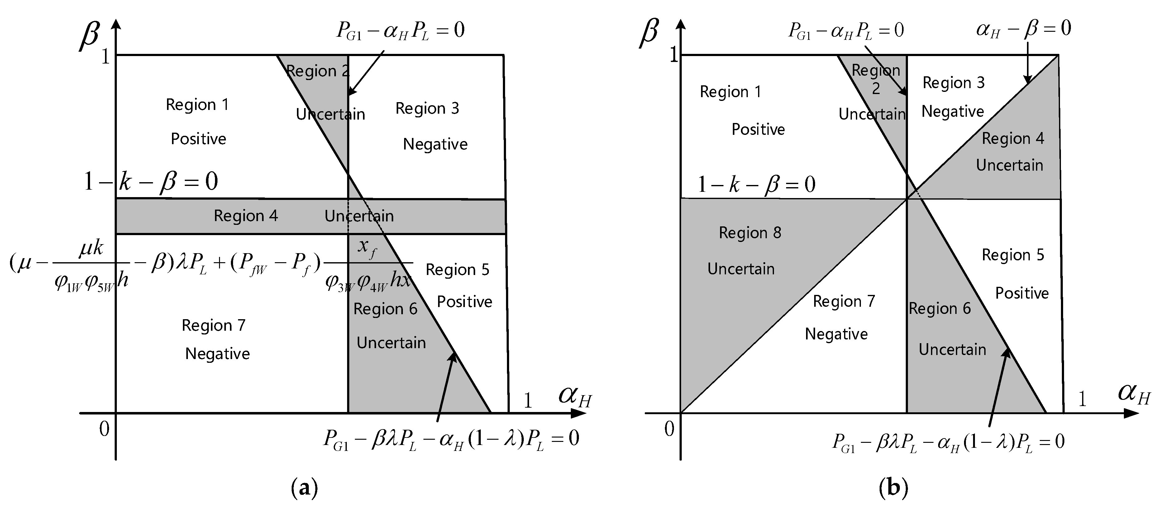
4.2. The Transient Stability Analysis of DFIG Integration Considering the Fault Location Factor

To analyze the influence of DFIG integration and fault location on transient stability, we take the case that the swing direction of rotor angle remains positive with and without DFIG integration. According to the definitions provided in Section 2, the variations in acceleration power and deceleration power due to DFIG integration can be formulated as follows:

$$\left\{\begin{array}{l}\Delta P_{acc}=(\mu -{\displaystyle \frac{\mu k}{{\phi }_{1W}{\phi }_{5W}h}}-\beta )P_W+(P_{fW}-P_f){\displaystyle \frac{x_f}{{\phi }_{3W}{\phi }_{4W}hx}}\\ \Delta P_{dec}=(\beta +k-1)\gamma P_L\end{array}\right..$$

(49)

By analyzing the rotor angle swing direction determination (47) (48) and the variations in acceleration power and deceleration power (49), it can be concluded that the key variables influencing the transient angle stability include the active output imbalance coefficient, the inertia ratio, and the fault location. Since the fault location predominantly affects the electromagnetic power during fault, while the inertia ratio is mainly determined by the mechanical characteristics and configuration of the generators, these two factors exhibit no intrinsic direct correlation. Therefore, for the three variables, it is sufficient to analyze the ($\beta {-x}_f)$ and the ($\beta {-\alpha }_H)$ planes formed by the active output imbalance coefficient with the inertia ratio and the fault location, respectively. This enables the establishment of the transient stability assessment criterion for wind–thermal bundled systems considering fault location. Based on this analysis, two scenarios will be discussed.

(1) Scenario 1: keeping the fault location constant, the relationship between the synchronous generator output imbalance coefficient and inertia ratio is analyzed. This creates the ($\beta {-\alpha }_H)$ plane.

Case 1: $\beta >\mu -\mu k/{\phi }_{1W}{\phi }_{5W}h+x_f(P_{fW}-P_f)/\gamma P_L{\phi }_{3W}{\phi }_{4W}hx$, $\beta >1-k$.

According to (49), with a fixed fault clearance time, it consistently holds that $\mathsf{\Delta }{P}_{acc}<0, \mathsf{\Delta }{P}_{dec}>0$. Based on EEAC, the integration of DFIG reduces the acceleration area and increases the deceleration area, thereby contributing to an enhancement of transient angle stability.

Case 2: $\beta <\mu -\mu k/{\phi }_{1W}{\phi }_{5W}h+x_f(P_{fW}-P_f)/\gamma P_L{\phi }_{3W}{\phi }_{4W}hx$, $\beta <1-k$.

In contrast to Case 1, it consistently holds that $\mathsf{\Delta }{P}_{acc}>0, \mathsf{\Delta }{P}_{dec}<0$. The integration of DFIG increases the acceleration area and reduces the deceleration area, leading to a decrease in the transient angle stability.

Case 3: $(\mu -\mu k/{\phi }_{1W}{\phi }_{5W}h+x_f(P_{fW}-P_f)/\gamma P_L{\phi }_{3W}{\phi }_{4W}hx-\beta )(\beta -1+k)<0$

Under the condition that $\mathsf{\Delta }{P}_{acc}>0, \mathsf{\Delta }{P}_{dec}>0$ or $\mathsf{\Delta }{P}_{acc}<0, \mathsf{\Delta }{P}_{dec}<0$, the integration of DFIG increases both the acceleration area and the deceleration area. Nevertheless, since the derived expressions for $P_f$ and $P_{fW}$ consider only the periodic components of current and voltage, estimation errors are inevitable. Additionally, the limited precision of the DC power flow model prevents an exact quantification of the changes in acceleration and deceleration power. As a result, the overall effect of DFIG integration on transient stability remains uncertain.

Following the same principle, the swing direction of rotor angle remains negative with and without DFIG integration. The acceleration and deceleration power values in (49) should be taken with opposite signs. The same three cases discussed earlier are analyzed accordingly.

As discussed above, the ($\beta {-\alpha }_H)$ plane can be divided into seven regions by four straight lines, as shown in Figure 4a. In regions 2 and 6, the swing direction is changed, which makes it impossible to determine the effect of DFIG integration. In region 4, the lack of precision in quantifying the changes in acceleration and deceleration power prevents the assessment of transient stability changes. In all other regions, the impact of DFIG integration on transient stability can be assessed based on the proposed theoretical criterion.

Remark 1.

Ref. [10] supposes that the electromagnetic power of synchronous generator equals to zero during fault, The variations in electromagnetic power distribution during the fault period have been neglected, which has led to inaccuracies in certain scenarios and a reduction in the range of an assessable stability area. The stability assessment area of the method from [10] is shown in Figure 4b. The acceleration and deceleration power simultaneously increase or decrease in the areas enclosed by the lines ${\alpha }_H-\beta$ and $1-k-\beta$ The errors in the DC power flow model hinder the quantitative comparison of the changes in these areas, which results in a significant number of regions being unable to employ transient stability analysis. This paper tackles the problem by representing the fault as an equivalent power injection source and implementing an improved DC power flow method, from which an explicit expression for the electromagnetic power during the fault is derived. This process changes the differential equation of $∆\delta$ and the acceleration power from (28) to (41). As a result, the boundary for assessing transient stability variations changes from the line ${\alpha }_H-\beta$ in Figure 4b to the line $\left(\mu -\mu k/{\phi }_{1W}{\phi }_{5W}h-\beta \right)\gamma P_L+x_f(P_{fW}-P_f)/{\phi }_{3W}{\phi }_{4W}hx$ in Figure 4a. It is evident that considering the fault location minimizes the areas where stability assessments cannot be conducted.

(2) Scenario 2: Keeping the inertia ratio constant, the relationship between the imbalance coefficient and the fault location is analyzed to construct the $\left(\beta -x_f\right)$ plane. When the swing direction of rotor angle remains positive, the following two cases are analyzed:

Case 1: $x_f(P_{fW}-P_f)>(\beta -\mu +\mu k/{\phi }_{1W}{\phi }_{5W}h)\gamma P_L{\phi }_{3W}{\phi }_{4W}hx$, $\beta <1-k$, while $x_f$ increases.

An increase in $x_f$ indicates that the fault occurs progressively closer to the DFIG connection point. It follows from (31) and (37) that $d{Z}_{ff}/d{x}_f>d{Z}_{ffW}/d{x}_f>0$, which means Z_ff increases at a faster rate than Z_ffW. According to (30), $P_f$ and $P_{fW}$ both decrease as $x_f$ increases, with $P_f$ decreasing at a faster rate than $P_{fW}$. Consequently, $x_f(P_{fW}-P_f)$ gradually increases as $x_f$ increases. Based on EEAC, since $\mathsf{\Delta }{P}_{acc}>0, \mathsf{\Delta }{P}_{dec}<0$, the integration of the DFIG enhances acceleration area of the system, while the increase in the fault location $x_f$ further enlarges the acceleration area. This indicates that the closer the fault occurs to the DFIG connection point, the worse it is to the transient stability of the system.

Case 2: $x_f(P_{fW}-P_f)<(\beta -\mu +\mu k/{\phi }_{1W}{\phi }_{5W}h)\gamma P_L{\phi }_{3W}{\phi }_{4W}hx$, $\beta >1-k$, while $x_f$ decreases.

As $x_f$ decreases, which means the fault occurs closer to the load, the analysis of $P_f$ and $P_{fW}$ follows the opposite trend in Case 1. This indicates that as $x_f$ decreases, $x_f(P_{fW}-P_f)$ gradually decreases. It follows that $\mathsf{\Delta }{P}_{acc}<0, \mathsf{\Delta }{P}_{dec}>0$. Additionally, as the fault location occurs closer to the load, the acceleration area further decreases, which indicates that the fault occurring closer to the load enhances the transient stability of the system.

Based on the aforementioned analysis, the transient stability assessment criterion for each region in the $\left(\beta -x_f\right)$ plane is illustrated in Figure 5.

In summary, considering the imbalance coefficient, the inertia ratio, and the fault location, the transient stability assessment criterion established by these three variables can be visualized in Figure 6. Figure 4a corresponds to the blue horizontal cross-section of Figure 6, while Figure 5 represents the green vertical cross-section of Figure 6.

By modifying the strong assumption that the electromagnetic power of synchronous generator is zero during the fault, this paper enhances the transient stability criterion introduced in [10], thereby extending the assessment scope of transient stability variations with DFIG integration.

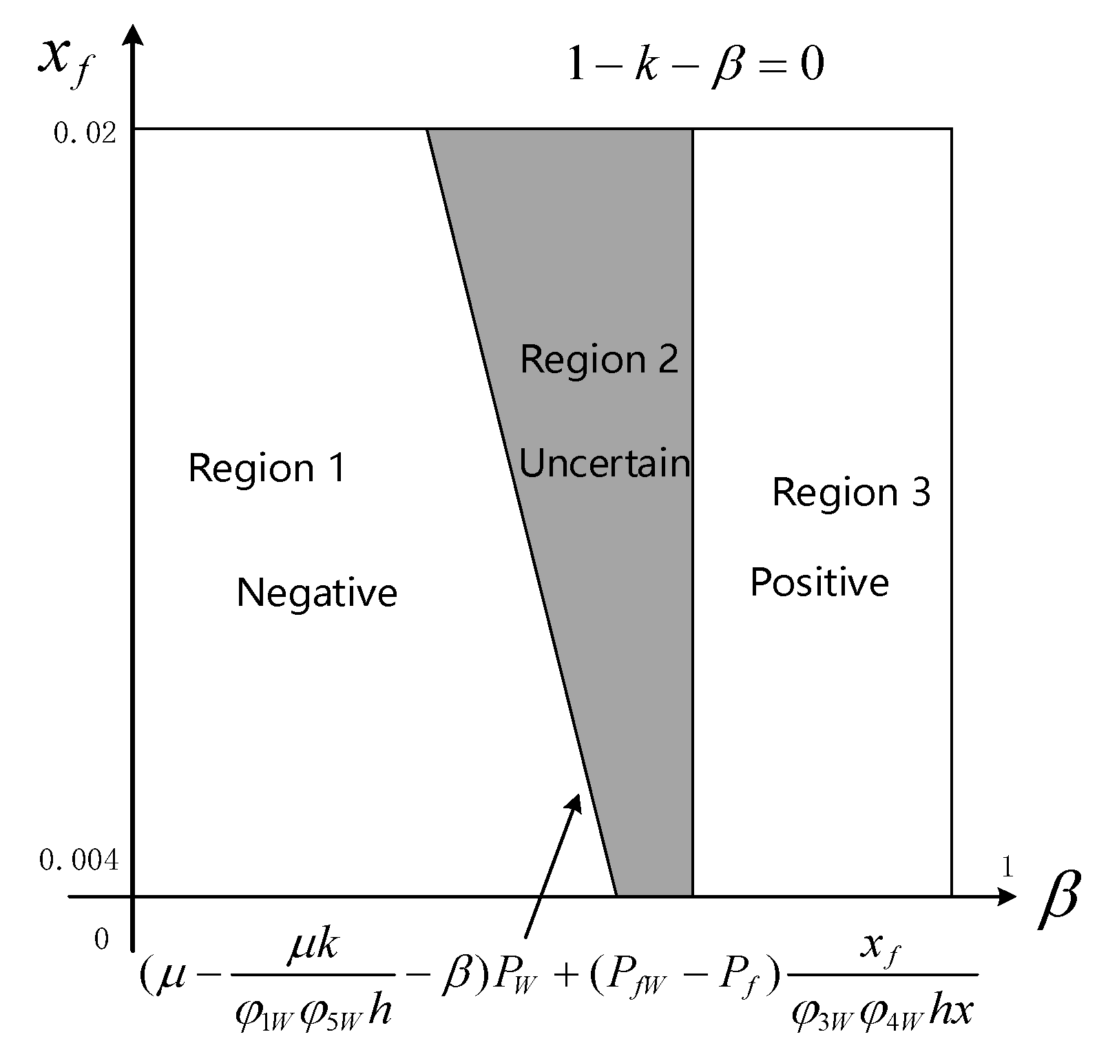
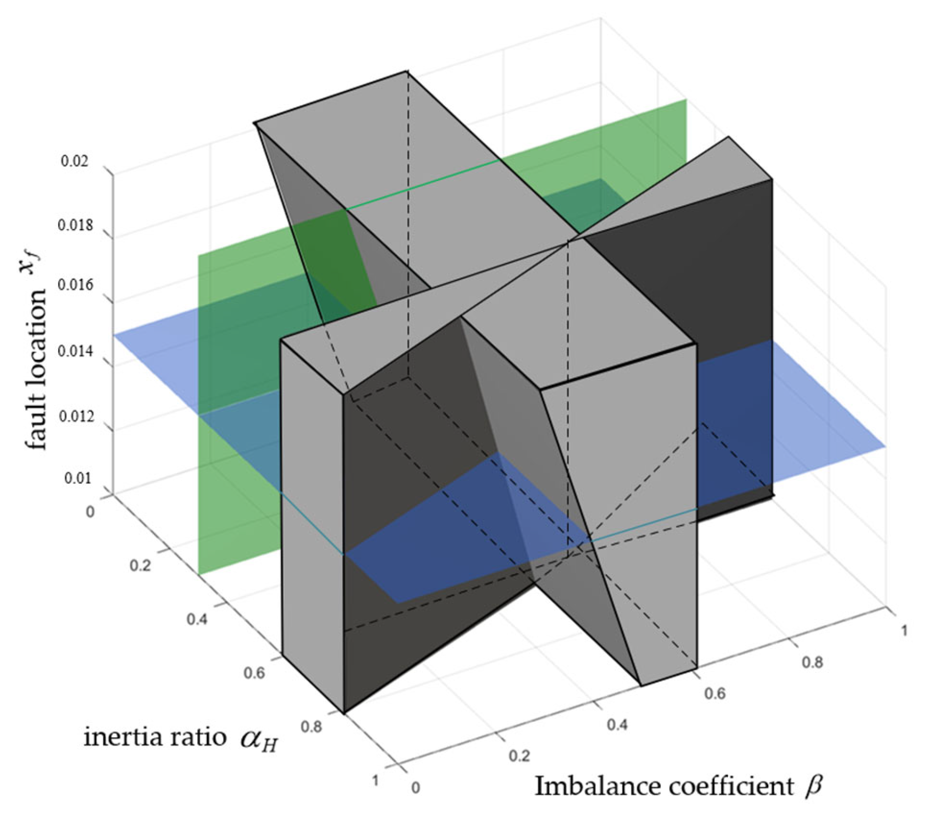
4.3. Impact Analysis of Fault Location Factors on the Transient Stability of the System with DFIG Integration

As derived in Section 3, it can be observed that the impact of fault location on the transient stability is confined to the rotor motion equation of the system during fault. This indicates that changes in fault location affect only the transient characteristics of the synchronous generator during fault, without impacting its dynamic behavior either before the fault occurs or after it has been cleared.

For the double-generator system with DFIG integration, it follows from (38) that when the swing direction of rotor angle is positive, the acceleration power of the OMIB system is given by

$$P_{accW}=P_{G1}-{\displaystyle \frac{\delta }{hx}}-P_L{\displaystyle \frac{{\phi }_{3W}(x-x_L)}{{\phi }_{2W}hx}}+(\mu -{\displaystyle \frac{\mu k}{{\phi }_{1W}{\phi }_{5W}h}}-\beta )P_W+P_{fW}{\displaystyle \frac{x_f}{{\phi }_{3W}{\phi }_{4W}hx}}-{\alpha }_T(1-{\phi }_{3W}^2)P_L.$$

(50)

We consider the fact that the voltage magnitude at the fault node is much smaller than that at the other nodes, i.e., ${\phi }_{4W}\ll {\phi }_{cW}, 4\notin c$. Consequently, in (50), it is sufficient to analyze the overall variation $x_f{P}_{fW}$ with respect to $x_f$ in order to obtain the effect of fault location factors on the transient stability of the system. The changes in the remaining terms concerning $x_f$ are not significantly relevant and can be disregarded.

According to (13), under the condition of a constant transitional resistance $R_g$, the magnitude of $P_{fW}$ depends solely on the self-impedance Z_ffW at the fault node. When the fault is assumed to take place at the outlet of the sending-end line, which means $x_L>kx>x_f$. Consequently, the imaginary component of Z_ffW becomes negligible. Differentiating Z_ffW with respect to $x_f$ yields

$${\displaystyle \frac{d{Z}_{ffW}}{d{x}_f}}=1+{\displaystyle \frac{2x_f}{kx-x_L}}>0.$$

(51)

Equation (51) indicates that the magnitude of Z_ffW increases with $x_f$, which means that the equivalent fault injected power $P_{fW}$ decreases in absolute value as $x_f$ increases. Since $P_{fW}$ is inherently negative, $P_{fW}$ increases with $x_f$. Considering that $x_f$ changes at a slower rate than $P_{fW}$ and its variation range is relatively small, $x_f{P}_{fW}$ increases overall as $x_f$ increases. According to EEAC, an increase in $x_f$ leads to an increase in the acceleration power of the system, while the deceleration power remains unaffected by the fault location, thereby worsening the transient stability of the system. The physical interpretation is that in a double-generator system with DFIG integration, when the swing direction of rotor angle is positive, transient angle stability is worse when the fault occurs near the DFIG connection point and better when it occurs near the load.

When the swing direction of rotor angle is negative, the acceleration power should be taken as the opposite of (50), which can be expressed as

$$P_{accW}=-P_{G1}+{\displaystyle \frac{\delta }{hx}}+P_L{\displaystyle \frac{{\phi }_{3W}(x-x_L)}{{\phi }_{2W}hx}}-(\mu -{\displaystyle \frac{\mu k}{{\phi }_{1W}{\phi }_{5W}h}}-\beta )P_W-P_{fW}{\displaystyle \frac{x_f}{{\phi }_{3W}{\phi }_{4W}hx}}+{\alpha }_T(1-{\phi }_{3W}^2)P_L.$$

(52)

The overall analysis of $x_f{P}_{fW}$, with respect to $x_f,$ follows the same principles as the previous discussion, which leads to an inverse relationship in the change in acceleration power. $x_f{P}_{fW}$ increases with $x_f$, leading to a decrease in acceleration power. This indicates that as $x_f$ increases, the transient stability of the system improves. Physically, this means that transient angle stability is better when the fault occurs near the DFIG connection point and worse when it occurs near the load.

To compare the impact of fault location on transient stability with and without DFIG integration, the influence of fault location on the stability of the double-generator system without DFIG integration is analyzed. From (32), when the swing direction of rotor angle is positive, the acceleration power of the system is given by

$$P_{acc}=P_{G1}-{\displaystyle \frac{\delta +\frac{{\phi }_3}{{\phi }_2}{P}_L(x-x_L)-P_f\frac{x_f}{{\phi }_3{\phi }_4}}{\frac{x_L}{{\phi }_1{\phi }_4}+\frac{x-x_L}{{\phi }_2{\phi }_3}}}-{\alpha }_T(1-{\phi }_3^2)P_L.$$

(53)

According to the expression of Z_ff, it generally holds that $x_L>x_f$. Similarly, differentiating Z_ff with respect to $x_f$ yields

$${\displaystyle \frac{d{Z}_{ff}}{d{x}_f}}=1-{\displaystyle \frac{2x_f}{x_L}}>0.$$

(54)

Equation (54) indicates that Z_ff increases with $x_f$, which in turn causes $x_f{P}_f$ to increase as well. As a consequence, the acceleration power of the system increases, implying that transient angle stability becomes worse as $x_f$ increases. Physically, this suggests that when the rotor angle of the system swings to the positive, the transient angle stability is better when the fault occurs near the synchronous generator, and worse when it occurs near the load.

When the swing direction of the rotor angle is negative, the acceleration power should be taken as the opposite of (53). Physically, this implies that transient angle stability is better when the fault occurs near the load, and worse when it occurs near the synchronous generator.

In summary, the qualitative analysis rules for the impact of fault location on transient stability of the system are presented in

Table 2. Relationship between the transient stability of the system and the fault location.

Swing Direction of Rotor Angle Condition	Condition of DFIG Integration	The Change in Fault Location	The Change in Transient Stability
The swing direction of the rotor angle is positive	Without DFIG integration	The load→the synchronous generator	Decrease
	With DFIG integration	The load→the DFIG connection point	Decrease
The swing direction of the rotor angle is negative	Without DFIG integration	The load→the synchronous generator	Increase
	With DFIG integration	The load→the DFIG connection point	Increase

.

4.4. Impact Analysis of the Line Impedance Between DFIG and the Synchronous Generator on the Transient Stability of the System

The line impedance between the DFIG and the synchronous generator is incorporated into the transient stability analysis model developed in this paper. The DFIG connection location ratio k denotes the proportion of the electrical distance from the DFIG connection point to G1 relative to the electrical distance between G1 and G2. kx represents the line impedance between the DFIG and G1. With DFIG integration, it is assumed that the electrical distance from the DFIG connection point to G1 is less than the distance from the load to G1.

When the swing direction of rotor angle is positive with DFIG integration, the acceleration power of the system during fault and the deceleration power after fault clearance typically satisfy the following relationship:

$$\left\{\begin{array}{c}{P}_{accW}=P_{G1}-{\displaystyle \frac{\delta }{hx}}-P_L{\displaystyle \frac{{\phi }_{3W}(x-x_L)}{{\phi }_{2W}hx}}+(\mu -{\displaystyle \frac{\mu k}{{\phi }_{1W}{\phi }_{5W}h}}-\beta )P_W+P_{fW}{\displaystyle \frac{x_f}{{\phi }_{3W}{\phi }_{4W}hx}}-{\alpha }_T(1-{\phi }_{3W}^2)P_L\\ P_{dec}=\left|P_{mW}-P_{eW}^C\right|=-P_{G1}+{\displaystyle \frac{\delta }{x^C}}-(1-k-\beta )\gamma P_L+{\displaystyle \frac{P_L(x^C-x_L^C)}{x^C}}\end{array}\right..$$

(55)

From (55), it is observed that the line impedance between DFIG and the synchronous generator influences both the acceleration and deceleration power of the system. The expression of hx in (55) is

$$hx={\displaystyle \frac{kx}{{\phi }_{1W}{\phi }_{5W}}}+{\displaystyle \frac{x_L-kx}{{\phi }_{4W}{\phi }_{5W}}}+{\displaystyle \frac{x-x_L}{{\phi }_{2W}{\phi }_{3W}}},$$

(56)

where ${\phi }_{4W}{\phi }_{5W}\ll {\phi }_{1W}{\phi }_{5W}$, since when k increases, hx decreases overall, so $\delta /hx$ increases, $P_L{\phi }_{3W}(x-x_L)/{\phi }_{2W}hx$ increases, and the rate of change in h is faster than k, $k/{\phi }_{1W}{\phi }_{5W}h$ decreases, and $P_{fW}{x}_f/{\phi }_{3W}{\phi }_{4W}hx$ increases. On the whole, the acceleration power decreases during the fault and the deceleration power increases after the fault is cleared. According to EEAC, the transient angle stability will be better as k increases.

When the swing direction of the rotor angle is negative, both the acceleration power and deceleration power are the opposite of those given by (55). In this case, as k increases, the acceleration power increases, and the deceleration power decreases, thus worsening the transient angle stability of the system.

5. Simulation Results and Discussion

In order to verify the transient rotor angle stability criterion proposed with DFIG integration, a simulation model was constructed on the MATLAB/Simulink platform, as shown in Figure 7. The synchronous generators are modeled using an eight-order system, with the rated power of G1 set at 300 MW and G2 at 200 MW. The load capacity for L1 and L2 are 180 MW and 320 MW, respectively, modeled using a constant impedance model, with a total load of 500 MW.

As shown in Figure 7, the connection point of DFIG is located at node 3, with the connection location ratio k = 38.95%. The DFIG model consists of components such as the RSC and GSC modules, among others. Under steady-state conditions, the DFIG active power output is 125 MW, corresponding to a wind power penetration of $\gamma =25\%$. A three-phase short circuit fault is simulated at the 50% point between nodes 3 and 4, starting at 0.5 s, with a fault duration of 0.2 s.

To verify the effectiveness of the proposed method, the energy integral metric V of the equivalent electromagnetic power against simulation results is evaluated under varying inertia and imbalance coefficients. The test trajectories are shown in Figure 8, and the computed metric values V are listed in

Table 3. Comparison of energy integral metrics V (p.u.).

Scenarios	Simulator Benchmark	Our Approximate	[10]’s
(a)	−0.021	−0.032	0
(b)	−0.074	−0.098	0
(c)	0.041	0.024	0
(d)	−0.048	−0.063	0

. The simulation results align closely with the theoretical values derived from (36), validating the rationality of modeling the fault as an equivalent power injection source.

From Figure 8 and Table 3, while the proposed method struggles to precisely match the electromagnetic power trajectory, its energy integral approximation remains close to the actual value. This suggests its applicability for subsequent EEAC analysis.

5.1. Verification of the System Transient Stability Criterion

To validate the transient stability criterion illustrated in Figure 4a, a series of batch simulations were conducted by varying $({\alpha }_H,\beta )$. ${\alpha }_H$ was systematically varied within the range [0.1, 0.9], while $\beta$ was systematically varied within the range [0, 1]. The simulation results are presented in Figure 9.

In Figure 9a, the horizontal axis represents the inertia ratio ${\alpha }_H$, while the vertical axis indicates the imbalance coefficient β. For each simulation scenario, the “+” is assigned if the actual simulation shows that DFIG integration enhances the transient angle stability of the system; otherwise, the “−” is assigned. When the theoretical criterion predicts that the integration of DFIG has a positive impact on the transient angle stability, the “○” is marked; when predicting a negative impact, the “□” is marked. Scenarios where the theoretical criterion is inconclusive remain unmarked. In summary, a scenario marked as “⊕” or “” signifies that the theoretical assessment is consistent with the simulation results. Additionally, a comparative analysis with the method proposed in ref. [10] is shown in Figure 9b.

As shown in Figure 9a, a total of 357 simulation cases were examined. The proposed stability criterion successfully incorporated 241 cases into the transient angle stability assessment, with only 7 cases exhibiting deviations between theoretical predictions and simulation results, achieving a theoretical accuracy of 234/241 = 97.09%. Meanwhile, 116 cases remained indeterminate under the proposed criterion. In contrast, the method in ref. [10] resulted in 151 undetermined cases and 8 incorrect cases, leading to an accuracy of 198/206 = 96.1%. It is observed that the method proposed in this paper not only increases the number of cases that can be assessed, but also improves the overall accuracy of the criterion, which indicates that the method can accurately identify stability boundaries and validate its rationality.

Similarly, to validate the stability criterion presented in Figure 5, batch simulations were conducted by varying $(\beta ,x_f)$. The simulation results are presented in Figure 10.

As shown in Figure 10, a total of 189 simulation cases were examined. The proposed criterion successfully incorporates 138 cases into the transient angle stability analysis, Theoretical predictions exhibited consistency with simulation results in 135 of these cases, with only three instances of deviation, leading to an analytical accuracy of 97.83%.

Based on the assumption of an equivalent power injection representation for DFIG, the impact of different wind power penetration levels on the accuracy of the theoretical criterion was simulated. The wind power penetration level was set to 15%, 20%, 25%, and 30%, while keeping the DFIG connection point unchanged. For each penetration level, batch simulations were conducted by systematically varying $({\alpha }_H,\beta ,x_f)$. The accuracy of transient stability criterion under different penetration levels is provided in

Table 4. Statistical results of the accuracy of the proposed transient stability judgment rules under different wind power penetration levels.

The Wind Power Penetration Level	The Change in Stability
15%	97.09%
20%	96.64%
25%	97.29%
30%	96.79%

.

Due to the inherent simplifications of the DC power flow model, modifications in the wind power penetration level are directly reflected in variations in the active output of DFIG and generators. The transient stability assessment accuracy across different wind penetration levels, as presented in Table 4, reveals that under the assumption of an equivalent power injection model of DFIG, deviations arising from different wind power penetration level and the system scales introduce minor discrepancies in the equivalent DFIG model. Nonetheless, these discrepancies do not exhibit a significant impact on the accuracy of the transient stability criterion framework.

5.2. Verification of the Impact of Fault Location Factors on System Transient Stability with DFIG Integration

To evaluate the impact of fault location on the transient stability of the system, different fault locations were set in with and without DFIG integration conditions. Under steady-state conditions, DFIG delivers an active power output of 125 MW, with a wind power penetration of 25%. A three-phase short-circuit fault is simulated at 0.5 s with a duration of 0.2 s. The fault locations were set at 10%, 50%, and 90% along the transmission line between nodes 3 and 4.

Figure 11 presents the curve of rotor angle between the two synchronous generators under various fault locations and system configurations. Without DFIG integration, Curve ① corresponds to the fault occurring at 90% of the transmission line between nodes 3 and 4, which is closer to the load. Curve ② corresponds to the fault occurring at 50% of the line, while Curve ③ represents the fault at 10% of the line, closer to the synchronous generator. With the integration of DFIG, Curve ④ shows the rotor angle for the fault at 90% of the line, closer to the load. Curve ⑤ corresponds to the fault at 50% of the line, and Curve ⑥ represents the fault at 10% of the line, closer to the DFIG connection point.

In Figure 11a,b, the rotor angle has a positive swing with and without DFIG integration. Without DFIG integration, the first-swing amplitude of the rotor angle difference increases progressively from Curves ① to ③, with Curve ③ displaying the largest amplitude. This indicates that transient stability of the system becomes weaker when the fault occurs closer to the synchronous generator. With DFIG integration, the first-swing amplitude of the rotor angle difference also increases from Curves ④ to ⑥, with Curve ⑥ showing the highest amplitude, suggesting the transient angle stability of the system is weaker when the fault occurs closer the DFIG connection point. These findings are consistent with theoretical derivations.

In Figure 11c,d, where rotor angle of the synchronous generators remains negative swing with and without DFIG integration, the first-swing amplitude of the rotor angle decreases progressively from Curves ① to ③, with Curve ① exhibiting the largest amplitude. This implies that the transient stability of the system is weaker when the fault occurs closer to the load. A similar trend is observed with DFIG integration, where the first-swing amplitude similarly diminishes, with Curve ⑥ exhibiting the most significant amplitude. This confirms that the transient stability of the system remains weaker when the fault is closer to the load.

Additionally, in Figure 11a,d, the overall first-swing amplitudes of Curves ④ to ⑥ are consistently higher than those of Curves ① to ③, indicating that DFIG integration weakens the transient angle stability. Conversely, in Figure 11b,c, the overall first-swing amplitudes of Curves ④ to ⑥ are consistently lower than those of Curves ① to ③, suggesting an enhancement in transient stability due to DFIG integration. These findings align with the proposed theoretical stability criterion.

Multi-scenario simulations are performed by varying (${\alpha }_H,\beta$), with each set of (${\alpha }_H,\beta$) representing a separate scenario. In each scenario, the fault location $x_f$ is incrementally increased, bringing it progressively closer to the wind farm connection point. The actual transient stability of the system is represented by the first swing amplitude of the angular difference between the two synchronous generators. The influence of increasing fault location on transient stability is evaluated by comparing the first swing amplitudes associated with various fault locations. The results of the simulations are presented in Figure 12.

Each point in Figure 12 represents a distinct scenario. In each scenario, if the first swing amplitude of the angular difference decreases monotonically with an increase in $x_f$, it indicates that the transient stability of the system improves monotonically with an increase in $x_f$, and a red “+” is marked at that point. Conversely, if the transient stability of the system weakens monotonically as $x_f$ increases, a blue “-” is placed. Similarly, if the theoretical criterion indicates that an increase in $x_f$ enhances the transient stability of systems, a blue circle is marked; otherwise, a red square is marked. According to Figure 12, a total of 357 scenarios are analyzed, with consistent results between the theoretical criterion judgments and simulations found in 345 scenarios, while 12 scenarios showed discrepancies, resulting in an accuracy rate of 96.66%.

5.3. Verification of the Impact of the Transmission Line Impedance Between DFIG and the Synchronous Generator on System Transient Stability with DFIG Integration

To validate the impact of the transmission line impedance between DFIG and the synchronous generator on transient stability of the system, simulations were conducted with varying DFIG connection location ratio k of 35%, 39%, and 43%. Figure 13a,b illustrate the curves of rotor angle when the line impedance between the DFIG and the synchronous generator varies, under positive and negative swing conditions, respectively.

As shown in Figure 13a, when ${\alpha }_H=0.4, \beta =0.3$, the rotor angle swing direction of the synchronous generators remains positive with the DFIG integration. As the DFIG connection location ratio k increases, corresponding to higher transmission line impedance between DFIG and the synchronous generator, this leads to a reduction in both the steady-state rotor angle difference and the first-swing amplitude. This suggests that a higher transmission line impedance contributes an enhancement to transient stability of the system.

Conversely, as shown in Figure 13b, when ${\alpha }_H=0.75, \beta =0.85$, the rotor angle swing direction of the synchronous generator remains negative with the DFIG integration. In this case, an increase in k leads to an enlargement in the steady-state rotor angle difference and a rise in the first-swing amplitude, indicating that a larger transmission line impedance negatively affects transient stability.

6. Conclusions

To address the difficulty of analytically characterizing the transient stability of power systems with DFIG integration, this paper improves upon the analytical method proposed in [10]. An explicit analytical approach is introduced which incorporates the fault location, based on the model of equivalent fault power injection. The simulation results confirm the following:

• By integrating the equivalent fault power injection source with the DC power flow-based transient stability assessment model, the assumption that the electromagnetic power of synchronous generator is zero during fault is relaxed. The proposed method incorporates fault location into transient stability analysis, effectively expanding the stability assessment criterion area of power system while maintaining accuracy.
• Without DFIG integration, when the swing direction of rotor angle is positive, the fault occurring closer to the generator leads to worse transient stability; conversely, the transient stability is worse when the fault occurs near the load when the swing direction of rotor angle is negative. With DFIG integration, the transient stability is worse when the fault occurs near the DFIG connection point in positive swing and near the load in negative swing.

The proposed method offers potential applications in weak-point identification, contingency analysis, wind farm planning, and generates critical stability operation scenarios. However, this paper does not account for the impact of grid-formed converters in renewable energy on transient stability, which will be a key area of future research.

Meanwhile, the current model emphasizes symmetrical faults and does not explicitly resolve the contributions of asymmetrical fault components. In future research, we plan to integrate the symmetrical component method into our framework to decouple and analyze scenarios associated with asymmetrical faults. This expansion will leverage the proposed analytical criteria as a basis and will combine it with sequence network analysis to tackle unbalanced faults.

Lastly, given the concerns about the accuracy of the DC power flow and fault equivalent power source models, the errors related to the method proposed in this study require further refinement. At the same time, while the stability assessment criterion can be utilized for the preliminary identification of instability boundaries, it is less capable of precise boundary characterization. Future investigations will consider the incorporation of artificial intelligence techniques to address this issue.

References

1. Khoa, N.M.; Van, N.T.H.; Hung, L.K.; Tuan, D.A. Investigation of the Impact of Large-Scale Wind Power and Solar Power Plants on a Vietnamese Transmission Network. Int. J. Renew. Energy Dev. 2022, 11, 863–870. [Google Scholar] [CrossRef]
2. Hadavi, S.; Mansour, M.Z.; Bahrani, B. Optimal Allocation and Sizing of Synchronous Condensers in Weak Grids With Increased Penetration of Wind and Solar Farms. IEEE J. Emerg. Sel. Top. Circuits Syst. 2021, 11, 199–209. [Google Scholar] [CrossRef]
3. Shair, J.; Li, H.; Hu, J.; Xie, X. Power System Stability Issues, Classifications and Research Prospects in the Context of High-Penetration of Renewables and Power Electronics. Renew. Sustain. Energy Rev. 2021, 145, 111111. [Google Scholar] [CrossRef]
4. Zhuo, Z.; Zhang, N.; Xie, X.; Li, H.; Kang, C. Key Technologies and Developing Challenges of Power System with High Proportion of Renewable Energy. Autom. Electr. Power Syst. 2021, 45, 171–191. [Google Scholar]
5. Shabani, H.R.; Hajizadeh, A.; Kalantar, M.; Lashgari, M.; Nozarian, M. Transient Stability Analysis of DFIG-Based Wind Farm-Integrated Power System Considering Gearbox Ratio and Reactive Power Control. Electr. Eng. 2023, 105, 3719–3735. [Google Scholar] [CrossRef]
6. Chakraborty, A.; Kumar, S.; Tudu, B.; Mandai, K.K. Analyzing the Dynamic Behavior of a DFIG-Based Wind Farm under Sudden Grid Disturbances. In Proceedings of the 2017 International Conference on Intelligent Sustainable Systems (ICISS), Palladam, India, 7–8 December 2017; pp. 336–341. [Google Scholar]
7. Soued, S.; Ramadan, H.S.; Becherif, M. Effect of Doubly Fed Induction Generator on Transient Stability Analysis under Fault Conditions. Energy Procedia 2019, 162, 315–324. [Google Scholar] [CrossRef]
8. Yousefian, R.; Bhattarai, R.; Kamalasadan, S. Transient Stability Enhancement of Power Grid With Integrated Wide Area Control of Wind Farms and Synchronous Generators. IEEE Trans. Power Syst. 2017, 32, 4818–4831. [Google Scholar] [CrossRef]
9. Ma, Y.; Zhu, D.; Zhu, H.; Hu, J.; Zou, X.; Kang, Y. Transient Stability Analysis and Enhancement of DFIG-Based Wind Turbine with Demagnetization Control during Grid Fault. IEEE Trans. Ind. Appl. 2025, 61, 1031–1042. [Google Scholar] [CrossRef]
10. Tang, L.; Shen, C.; Zhang, X. Impact of Large-scale Wind Power Centralized Integration on Transient Angle Stability of Power Systems-Part I: Theoretical Foundation. Pro. CSEE 2015, 35, 3832–3842. [Google Scholar]
11. Tang, L.; Shen, C.; Zhang, X. Impact of Large-scale Wind Power Centralized Integration on Transient Angle Stability of Power Systems-Part II: Factors Affecting Transient Angle Stability. Pro. CSEE 2015, 35, 4043–4051. [Google Scholar]
12. Ge, X.; Qian, J.; Fu, Y.; Lee, W.-J.; Mi, Y. Transient Stability Evaluation Criterion of Multi-Wind Farms Integrated Power System. IEEE Trans. Power Syst. 2022, 37, 3137–3140. [Google Scholar] [CrossRef]
13. Hamilton, R.I.; Papadopoulos, P.N. Using SHAP Values and Machine Learning to Understand Trends in the Transient Stability Limit. IEEE Trans. Power Syst. 2024, 39, 1384–1397. [Google Scholar] [CrossRef]
14. Yang, S.; Li, B.; Hao, Z.; Hu, Y.; Xie, H.; Zhao, T.; Zhang, B. Multi-Swing Transient Stability of Synchronous Generators and IBR Combined Generation Systems. IEEE Trans. Power Syst. 2025, 40, 1144–1147. [Google Scholar] [CrossRef]
15. Ahmed, S.D.; Al-Ismail, F.S.M.; Shafiullah, M.; Al-Sulaiman, F.A.; El-Amin, I.M. Grid Integration Challenges of Wind Energy: A Review. IEEE Access 2020, 8, 10857–10878. [Google Scholar] [CrossRef]
16. Liu, S.; Li, G.; Zhou, M. Power System Transient Stability Analysis with Integration of DFIGs Based on Center of Inertia. CSEE J. Power Energy Syst. 2016, 2, 20–29. [Google Scholar] [CrossRef]
17. Xue, Y.; Van Custem, T.; Ribbens-Pavella, M. Extended Equal Area Criterion Justifications, Generalizations, Applications. IEEE Trans. Power Syst. 1989, 4, 44–52. [Google Scholar] [CrossRef]
18. Bahmanyar, A.; Ernst, D.; Vanaubel, Y.; Gemine, Q.; Pache, C.; Panciatici, P. Extended Equal Area Criterion Revisited: A Direct Method for Fast Transient Stability Analysis. Energies 2021, 14, 7259. [Google Scholar] [CrossRef]
19. Ying, J.; Yuan, X.; Hu, J. Inertia Characteristic of DFIG-Based WT Under Transient Control and Its Impact on the First-Swing Stability of SGs. IEEE Trans. Energy Convers. 2017, 32, 1502–1511. [Google Scholar] [CrossRef]
20. Molina-Moreno, I.; Medina, A.; Cisneros-Magaña, R.; Anaya-Lara, O. Harmonic and Transient State Assessment in the Time-Domain. In Proceedings of the 2016 IEEE International Autumn Meeting on Power, Electronics and Computing (ROPEC), Ixtapa, Mexico, 9–11 November 2016; pp. 1–6. [Google Scholar]
Figure 1. The double-generator system with DFIG integration.
Electronics 14 01526 g001
Figure 2. Analysis diagram of the fault node.
Electronics 14 01526 g002
Figure 3. Diagram of the location of the short-circuit fault.
Electronics 14 01526 g003
Figure 4. Impact of the imbalance coefficient and inertia ratio on transient stability with DFIG integration. (a) Visualization of transient stability analysis rules considering fault factors; (b) comparison of the method in ref. [10].
Electronics 14 01526 g004
Figure 5. Impact of the imbalance coefficient and the fault location on transient stability with DFIG integration.
Electronics 14 01526 g005
Figure 6. Schematic diagram of the relationship between changes in transient stability and variations in the imbalance coefficient, the inertia ratio, and the fault location with DFIG integration.
Electronics 14 01526 g006
Figure 7. Topology of double-generator system with DFIG integration.
Electronics 14 01526 g007
Figure 8. Comparison between the equivalent electromagnetic power and the simulation trajectory during fault period. (a) α H = 0.4 ,     β = 0.3 ; (b) α H = 0.4 ,     β = 0.85 ; (c) α H = 0.75 ,     β = 0.3 ; (d) α H = 0.75 ,     β = 0.85 .
Electronics 14 01526 g008
Figure 9. Comparison of theoretical analysis and simulation of inertia ratio and imbalance coefficient on transient stability with DFIG integration. (a) The method proposed in this paper; (b) comparison of the method in ref. [10].
Electronics 14 01526 g009
Figure 10. Comparison of theoretical analysis and simulation results of fault location and imbalance coefficient on transient stability with DFIG integration.
Electronics 14 01526 g010
Figure 11. The trajectory of rotor angle under the faults at different locations under different conditions. (a) α H = 0.4 ,     β = 0.3 ; (b) α H = 0.4 ,     β = 0.85 ; (c) α H = 0.75 ,     β = 0.3 ; (d) α H = 0.75 ,     β = 0.85 .
Electronics 14 01526 g011aElectronics 14 01526 g011b
Figure 12. The impact of fault location on transient stability related to the imbalance coefficient and inertia ratio.
Electronics 14 01526 g012
Figure 13. The trajectory of rotor angle under different line impedance between wind farms and the bus of thermal power plants in different conditions. (a) α H = 0.4 ,     β = 0.3 ; (b) α H = 0.75 ,     β = 0.85 .
Electronics 14 01526 g013