Abnormal Heart Sound Detection Using Common Spatial Patterns and Random Forests

Abstract

Early and accurate diagnosis of heart conditions is pivotal for effective treatment. Phonocardiography (PCG) has become a standard diagnostic tool for evaluating and detecting cardiac abnormalities. While traditional cardiac auscultation remains widely used, its accuracy is highly dependent on the clinician’s experience and auditory skills. Consequently, there is a growing need for automated, objective methods of heart sound analysis. This study explores the efficacy of the Common Spatial Patterns (CSP) feature extraction algorithm paired with the Random Forest (RF) classifier to distinguish between normal and pathological heart sounds. The signal is denoised, transformed, and segmented into fixed-length segments. CSP is applied to extract discriminative features (a set of Spatial Patterns), which are then fed into the classifier for cardiac diagnosis. The proposed method was evaluated using PhysioNet/CinC Challenge 2016 and Yaseen2018 (Heart Sound Murmur) datasets. On the testing set of the PhysioNet dataset, the RF classifier achieved 100% precision, recall, accuracy, F1 score, and AUC. Similarly, on the testing set of the Yaseen2018 dataset, it achieved 96.30% precision, 1.00 recall, 98.08% accuracy, 98.11% F1 score, and 99.41% AUC.

1. Introduction

Cardiovascular diseases (CVDs) remain the leading cause of mortality worldwide, accounting for an estimated 17.9 million deaths in 2019, which represents approximately 32% of all global deaths [1]. In the Kingdom of Saudi Arabia (KSA), the situation is particularly alarming, with 294 deaths per 100,000 population annually, where CVDs contribute to more than 45% of all fatalities [2,3]. Traditional diagnostic tools, such as echocardiography and electrocardiograms (ECGs), are effective but often require specialized equipment and trained personnel for accurate interpretation. This dependency on advanced technology and expertise restricts their accessibility, particularly in low-resource settings, where the need for timely and accurate diagnosis is critical. Therefore, there is an urgent demand for more accessible, cost-effective diagnostic methods that can be utilized widely. Heart sound analysis, a non-invasive and potentially scalable approach, offers a promising solution for the early detection and continuous monitoring of heart conditions. Raymond et al. [4] propose a method for heart sound classification aimed at detecting cardiovascular diseases with a minimal number of features to reduce computational load. The heart sounds were decomposed into three frequency bands, and Shannon entropy and spectral entropy were extracted from each band, resulting in six features that were then used as inputs for a support vector machine (SVM) classifier. Utilizing the PhysioNet Computing in Cardiology Challenge 2016 dataset, the SVM classifier achieved an accuracy of 82.5%, with sensitivity and specificity of 85% and 80%, respectively. This method demonstrates that effective heart sound classification is possible with fewer features, highlighting its potential for developing compact and efficient systems for remote health monitoring. Morshed et al. [5] present a method for diagnosing heart valve disorders using Phonocardiography (PCG) signals, employing an ensemble learning framework that integrates various machine learning models to enhance diagnostic accuracy. The approach combines time-domain and frequency-domain features, which are input into classifiers such as SVM, k-Nearest Neighbors (k-NN), and RF. This multi-model strategy capitalizes on the strengths of each classifier. Statistical and probabilistic features from the formant frequencies of PCG signals were used. By utilizing an ensemble of bagged tree classifiers, they achieved an accuracy of 93.46% for binary classification. Zeinali et al. [6] utilized heart sound data from the PhysioNet database, employed Genetic Algorithms (GA) for feature selection, and used Principal Component Analysis (PCA) and Linear Discriminant Analysis (LDA) for dimensionality reduction. Several machine learning classifiers, including SVM, Gradient Boosting Classifier (GBC), and RF, are used to classify heart sounds. The study achieved an accuracy of 98% for binary classification using the GBC. Fauzi et al. [7] proposed a method to classify the heart sound into normal and abnormal using empirical mode decomposition and first-order statistics. They applied their method on the PhysioNet Computing in Cardiology challenge 2016 dataset and achieved an accuracy of 98.2% using a k-NN classifier. Potes et al. [8] presented an approach for classifying the heart sound as normal and abnormal based on time-frequency domain features and the AdaBoost classifier. The approach obtained a sensitivity, specificity, and overall score of 94.24%, 77.81%, and 86.02%, respectively, using the PhysioNet/CinC Challenge 2016 dataset.

Among various techniques for feature extraction, Spatial Patterns (CSP) was initially developed for brain–computer interface (BCI) applications and demonstrated significant potential in extracting meaningful features from complex and noisy datasets. Recent advancements in CSP have shown that, with optimized implementations, it is possible to significantly outperform traditional approaches, achieving nearly a 10% improvement in classification accuracy in certain BCI tasks [9]. Therefore, it has found wide applications in different areas such as Parkinson disease detection [10], motor imagery brain–computer interface [11,12], myoelectric control [13], mental disease classification [14], and seizure detection and prediction [15,16].

In this study, we present a new approach for cardiac audio classification that is based on the CSP feature extraction technique and machine learning classifier. This algorithm finds spatial filters such that the variance of the filtered signal is maximal for one class and minimal for the other class. CSP enhances class discriminative power, making it an effective method for distinguishing among various heart conditions. To the best of our knowledge, this is the first time that CSP has been applied to heart sound classification using PCG signal.

The structure of the paper is as follows: Section 2 delves into the mathematical formulation of CSP. The methodology employed is outlined in Section 3. Section 4 details the experimental results, and concluding observations are discussed in Section 5.

2. Common Spatial Pattern

The CSP method, originally introduced by Koles et al. [17] for Electroencephalogram (EEG) analysis, is a statistical technique used to differentiate between normal and pathological conditions. In this study, CSP is applied to distinguish between normal and abnormal PCG signals. The mathematical formulation of the CSP approach is presented below [18].

Let X_ik ∈ R^NxS represent the ith segment of a PCG signal from class k (where k= 1 for normal and k = 2 for abnormal signals), with N denoting the number of channels and S representing the number of samples.

• We calculated the normalized covariance matrix C_k for class K,

  $${\mathit{C}}_{\mathit{k}}=({\displaystyle \frac{1}{\mathit{M}}}){\sum }_{\mathit{i}=1}^{\mathit{M}}{\displaystyle \frac{{\mathit{X}}_{\mathit{i}\mathit{k}}{\mathit{X}}_{\mathit{i}\mathit{k}}^{\mathit{T}}}{\mathit{t}\mathit{r}\mathit{a}\mathit{c}\mathit{e}\left({\mathit{X}}_{\mathit{i}\mathit{k}}{\mathit{X}}_{\mathit{i}\mathit{k}}^{\mathit{T}}\right)}},$$

  (1)

  where M is the number of signal segments, trace is the sum of the diagonal elements, and T denotes matrix transposition.
• We calculated the normalized covariance matrix C₀ for the remaining classes,

  $${\mathit{C}}_0=({\displaystyle \frac{1}{\mathit{M}(\mathit{L}-1)}}){\sum }_{\begin{array}{c}j=1\\ j\ne k\end{array}}^{\mathit{L}}{\sum }_{\mathit{i}=1}^{\mathit{M}}{\displaystyle \frac{{\mathit{X}}_{\mathit{i}\mathit{j}}{\mathit{X}}_{\mathit{i}\mathit{j}}^{\mathit{T}}}{\mathit{t}\mathit{r}\mathit{a}\mathit{c}\mathit{e}\left({\mathit{X}}_{\mathit{i}\mathit{j}}{\mathit{X}}_{\mathit{i}\mathit{j}}^{\mathit{T}}\right)}},$$

  (2)

  where L is the total number of classes.
• We computed the composite covariance matrix.

  $${\mathit{C}}_{\mathit{c}}={\mathit{C}}_{\mathit{k}}+{\mathit{C}}_0.$$

  (3)
• We applied singular value decomposition (SVD) on C_c to obtain the eigenvalues ψ and the normalized eigenvector matrix F_c.

  $${\mathit{C}}_{\mathit{c}=}{\mathit{F}}_{\mathit{c}}\mathit{\psi }{\mathit{F}}_{\mathit{C}}^{\mathit{T}}.$$

  (4)
• We applied a whitening transform to both covariance matrices, C_k and C₀, using the whitening matrix $\mathit{P}={\mathit{\psi }}^{-1}{\mathit{F}}_{\mathit{c}}^{\mathit{T}}$, leading to the transformed matrices D_k and D₀.

  $${\mathit{D}}_{\mathit{k}}=\mathit{P}{\mathit{C}}_{\mathit{k}}{\mathit{P}}^{\mathit{T}},{\mathit{D}}_0=\mathit{P}{\mathit{C}}_0{\mathit{P}}^{\mathit{T}}.$$

  (5)
• We decomposed D_k and D₀ using eigenvalue decomposition.

  $${\mathit{D}}_{\mathit{k}}=\mathit{U}{\mathsf{\Lambda }}_{\mathit{k}}{\mathit{U}}^{\mathit{T}},{\mathit{D}}_0=\mathit{U}{\mathsf{\Lambda }}_0{\mathit{U}}^{\mathit{T}}.$$

  (6)

Since D_k and D₀ share the same eigenvectors, their eigenvalues satisfy Λ_k + Λ₀ = I, where I is the identity matrix. Here, U is the matrix of eigenvectors, and Λ is the diagonal matrix of eigenvalues.

7.

We constructed the CSP projection matrix W_k.

$${\mathit{W}}_{\mathit{k}}={\left({\mathit{U}}^{\mathit{T}}\mathit{P}\right)}^{\mathit{T}}.$$

(7)

Each row of W_k represents a spatial filter, while each column of ${\mathit{W}}_{\mathit{K}}^{-1}$ corresponds to a spatial pattern. In Section 3.3, we showed how to utilize W_k to extract features.

3. Methodology

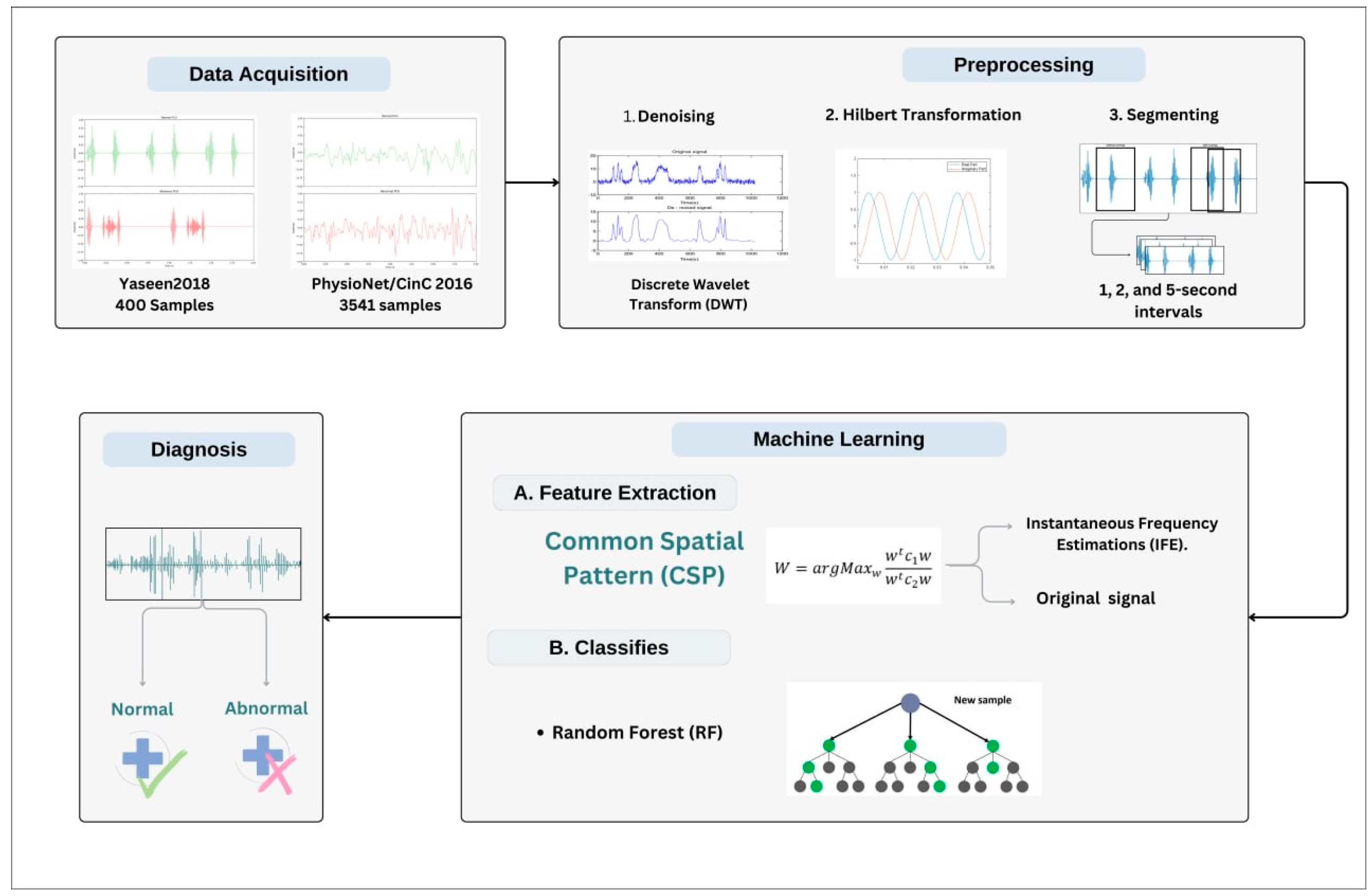
The proposed methodology consists of the following stages: data acquisition, data preprocessing, feature extraction, and classification. In the preprocessing stage, the PCG signal is denoised, Hilbert transformed, and segmented. Then, the features are extracted using the CSP algorithm. Finally, the extracted features will be used to train the classifier; the trained classifier is then tasked to predict the PCG, whether it is normal or abnormal. The schematic in Figure 1 illustrates the overall scheme of the proposed methodology. The details of each stage are provided in the following subsections.

3.1. Datasets

3.1.1. Yaseen2018 (Heart Sound Murmur Dataset)

The dataset utilized in this study is the Yaseen2018 (Heart Sound Murmur dataset), a publicly available heart sounds dataset. It contains 1000 audio clips with a maximum duration of 3 s. The data are categorized into five groups, each containing 200 clips. The dataset includes five primary classes: normal (N), aortic stenosis (AS), mitral stenosis (MS), mitral regurgitation (MR), and mitral valve prolapse (MVP), as illustrated in

Table 1. Number of segments using the Yaseen2018 dataset.

Dataset	1 s Segment Lenth	2 s Segment Lengh
Training	526	240
Testing	226	104

. The audio files are in *.wav format, sampled at 8000 Hz, and converted to a single channel [18].

For this study, the data were regrouped into two categories, normal and abnormal, to facilitate a binary classification. Specifically, the 200 audio clips from the normal class were designated as the normal category. Meanwhile, fifty randomly selected recordings from each of the other four classes (AS, MS, MR, and MVP) were combined to form the abnormal category. In this study, PCG signals were segmented into two different lengths: 1 and 2 s. The data were split into balanced training and testing sets at a 70/30 ratio.

3.1.2. PhysioNet/CinC Challenge 2016 Dataset

The PhysioNet/CinC challenge 2016 dataset [19] is widely used in the literature for developing an AI-based PCG signal classification system. The dataset consists of sound recordings collected during clinical trials at hospitals, comprising data from both children and adults. These recordings are categorized into two classes: healthy (normal) and pathological (abnormal). It was originally gathered from various sources using heterogeneous equipment, resulting in recordings sampled at different rates. To ensure consistency, compatibility, and optimal processing, all recordings were resampled to 2000 Hz, following the standard adopted by the authors. The training set comprises 3240 PCG recordings, with 2575 normal and 665 abnormal samples, while the validation set contains 301 recordings (151 normal and 150 abnormal). The recordings, originally in WAV format, were resampled to 2000 Hz and have varying durations from 5 to 120 s. In this study, PCG signals were segmented into three different lengths: 1, 3, and 5 s.

3.2. Preprocessing

During the preprocessing stage, three operations are carried out on the PCG signal: denoising, Hilbert transformation, and segmentation of the PCG signal. Given that heart sound recordings may contain various types of noise (e.g., respiratory sounds, ambient noise, stethoscope artifacts), an essential preprocessing step is to apply a technique such as wavelet transform to eliminate these unwanted components. The process begins by decomposing the noisy signal using the Discrete Wavelet Transform (DWT), which separates it into various frequency components across multiple levels. In this study, Daubechies wavelet with six vanishing moments is used, and the decomposition level is set to 4. A universal threshold, calculated from the median absolute deviation of the detail coefficients, is used to estimate the noise level [20]. Soft thresholding is applied to the wavelet detail coefficients to reduce noise without distorting the significant parts of the signal.

The signal is finally reconstructed from the modified coefficients, resulting in a cleaner, denoised version.

Since the CSP algorithm is designed for multichannel data, the Hilbert transform is applied to create an additional channel, $\widehat{X}\left(t\right)$, from the original PCG signal, X(t). This transformed signal, $\widehat{X}\left(t\right)$, is derived in the time domain by convolving the original signal, X(t), with the Hilbert transformer ${\displaystyle \frac{1}{\pi t}}$. The computation of this transformation is shown in Equation (8), assuming the integral is well-defined [21].

$$\widehat{\mathit{X}}\left(\mathit{t}\right)={\displaystyle \frac{1}{\mathit{\pi }}}{\int }_{-\mathit{\infty }}^{\mathit{\infty }}{\displaystyle \frac{\mathit{X}\left(\mathit{\tau }\right)}{\mathit{t}-\mathit{\tau }}}\mathit{d}\mathit{\tau }.$$

(8)

Equivalently, the signal $\widehat{\mathit{X}}\left(\mathit{t}\right)$ can be obtained by passing X(t) through a linear time-invariant system whose frequency response (the Fourier transform of 1/(πt)) is equal to –jsgn(f), where sgn(f) is the signum function.

Additionally, we computed the instantaneous frequency for both the original and transformed signals. Instantaneous frequency estimation (IFE) is one of the most commonly used time-frequency techniques and is applied across various fields, such as speech analysis, medical diagnostics, and communications. Instantaneous frequency estimation is used to capture the variation in frequency of a signal over time, making it particularly useful for analyzing non-stationary signals like PCG recordings, which exhibit temporal variations. The instantaneous frequency of a signal provides insight into how the frequency content evolves, which can be crucial for distinguishing between normal and abnormal heart sounds. The key benefit of using IFE is its ability to offer detailed time-frequency information, which is particularly valuable for analyzing PCG signals. Since heart sounds consist of both transient and periodic components, IFE allows us to capture subtle variations in heart sound patterns that might go unnoticed with traditional frequency-domain techniques.

The instantaneous frequency of a signal X(t) (PCG) is estimated as follows [22]:

• The power spectrum P(t,f) of the signal X(t) is computed.
• The instantaneous frequency is estimated as follows:

  $${\mathbf{X}}_{{\mathbf{i}\mathbf{n}\mathbf{s}\mathbf{t}}^{\left(\mathbf{t}\right)}}={\displaystyle \frac{{\int }_0^{\mathbf{\infty }}\mathbf{f}\mathbf{P}\left(\mathbf{t},\mathbf{f}\right)\mathbf{d}\mathbf{f}}{{\int }_0^{\mathbf{\infty }}\mathbf{P}\left(\mathbf{t},\mathbf{f}\right)\mathbf{d}\mathbf{f}}}$$

  (9)

Here, P(t,f) denotes the power spectral density at time t and frequency f. This approach ensures that the estimated frequency corresponds to the predominant spectral components at each time instant, providing a meaningful representation of the signal’s frequency variations over time.

Finally, the recordings are segmented into uniform intervals: 1 and 2 s segment lengths for the Yaseen2018 (Heart Sound Murmur) dataset and 1, 3, and 5 s segment lengths for the PhysioNet/CinC Challenge 2016 dataset, all without overlap (Table 1 and

Table 2. Number of segments using the PhysioNet/CinC Challenge 2016 dataset.

Dataset	1 s Segment Lenth	3 s Segment Lengh	5 s Segment Lengh
Training	3240	3240	3240
Testing	301	301	301

). Figure 2 illustrates an example of a normal and abnormal audio segment with a length of 3 s. The number of segments for both the training and testing datasets is also presented.

3.3. CSP-Based Feature Extraction

With the data preprocessed and segmented, the next step is feature extraction. CSP is employed to extract discriminative features from the heart sound recordings by identifying spatial filters that maximize the variance for one class while minimizing it for the other. In this study, CSP is applied to heart sound signals to capture features that highlight the differences between normal and abnormal heart sounds.

Feature extraction is a crucial step in the PCG classification process. It starts with constructing the projection matrix W_k. The training and testing feature vectors are obtained by projecting each PCG segment X (of size S × N) onto the matrix W_k (of size N × N), resulting in the transformed matrix B_k (of size N × S),

$${\mathit{B}}_{\mathit{k}}={\mathit{W}}_{\mathit{k}}{\mathit{X}}^{\mathit{T}},$$

(10)

where X represents a segment from either class. The feature vector ${\mathbf{f}}_{\mathbf{k}}$ for a given segment X is then computed as the log-variance of each row of matrix B_k.

$${\mathit{f}}_{\mathit{k}}=\mathit{l}\mathit{o}\mathit{g}\left(\mathit{v}\mathit{a}\mathit{r}\left({\mathit{B}}_{\mathit{k}}\right)\right).$$

(11)

CSP is applied to the multichannel data, which consists of the original PCG signal and its analytic signal, to extract four features. These features correspond to the log-variance of the CSP-filtered components, capturing the most discriminative Spatial Patterns. Additionally, four more features are extracted by applying CSP to the multichannel instantaneous frequency estimation, computed from the original PCG signal and its analytic signal. These features are also derived from the log-variance of the CSP-projected signals, ensuring robust class separation.

3.4. Classification

Once the features are extracted, they are then fed into a machine learning classifier to categorize the heart sounds into normal or pathological classes. In this study, an RF classifier was employed. RF, an ensemble learning method based on decision tree classifiers, was selected for its high accuracy and ability to handle complex datasets with non-linear relationships. RF combines multiple decision trees trained on various subsets of the training data and averages their predictions, improving the generalization capability and reducing the risk of overfitting. This method is particularly suitable for medical signal classification due to its robustness and interpretability. The number of trees (n = 100) and other hyperparameters were optimized through grid search to achieve the best performance on both datasets. The grid search optimization was performed separately for each dataset. The RF classification for a sample $\mathrm{X}$ is computed as follows:

$$\widehat{\mathit{y}}={\displaystyle \frac{1}{\mathit{T}}}{\sum }_{\mathit{t}=1}^{\mathit{T}}{\mathit{h}}_{\mathit{t}}\left(\mathit{x}\right).$$

(12)

Classification for a given sample $\mathit{X}$ is achieved by constructing an ensemble of decision trees and averaging their predictions. Specifically, each tree in the forest makes an independent prediction, denoted as ${\mathit{h}}_{\mathit{t}}\left(\mathit{x}\right)$, where $t$ represents the $t$-th tree. The final prediction, $\widehat{y}$, is obtained by averaging the predictions across all $\mathit{T}$ trees, which is the total number of trees in the forest. This averaging process reduces variance and enhances model robustness, making Random Forest particularly effective for handling complex datasets such as those with CSP-extracted heart sound features [23].

The classifier was trained on 70% of the dataset and tested on the remaining 30%, using 1, 3, and 5 s segment lengths for the PhysioNet/CinC Challenge 2016 dataset and 1 and 2 s segment lengths for the Yaseen2018 dataset. The classifier’s performance was evaluated using standard metrics, as detailed in the following section.

3.5. Performance Metrics

The classifier’s performance was assessed using standard metrics such as a confusion matrix, along with accuracy, precision, recall metrics, and AUC, offering a detailed understanding of the trade-offs among various evaluation criteria.

The confusion matrix categorizes classification outcomes into four groups: true positives (TP) and true negatives (TN) represent correctly classified positive and negative instances, respectively, while false positives (FP) and false negatives (FN) denote misclassified cases—FP refers to incorrectly predicted positives, and FN to incorrectly predicted negatives. The performance metrics were computed using the following equations [23]:

The accuracy evaluates the overall effectiveness of the classifier by determining the proportion of correctly classified instances relative to the total number of samples. It is computed as follows:

$$\mathit{A}\mathit{c}\mathit{c}\mathit{u}\mathit{r}\mathit{a}\mathit{c}\mathit{y}={\displaystyle \frac{\mathit{T}\mathit{P}+\mathit{T}\mathit{N}}{\mathit{T}\mathit{P}+\mathit{F}\mathit{N}+\mathit{T}\mathit{N}+\mathit{F}\mathit{P}}}.$$

(13)

Precision evaluates the reliability of positive predictions, representing the percentage of correctly identified positives among all predicted positives. It is given by the following:

$$\mathit{P}\mathit{r}\mathit{e}\mathit{c}\mathit{i}\mathit{s}\mathit{i}\mathit{o}\mathit{n}={\displaystyle \frac{\mathit{T}\mathit{P}}{\mathit{T}\mathit{P}+\mathit{F}\mathit{P}}}.$$

(14)

Recall (sensitivity) measures the classifier’s ability to identify actual positive instances, calculated as the ratio of true positives to the total number of actual positive cases.

$$\mathit{R}\mathit{e}\mathit{c}\mathit{a}\mathit{l}\mathit{l}={\displaystyle \frac{\mathit{T}\mathit{P}}{\mathit{T}\mathit{P}+\mathit{F}\mathit{N}}}.$$

(15)

The F1 score provides a harmonic mean of precision and recall, offering a balanced measure when both false positives and false negatives carry significant consequences. It is particularly useful in scenarios where an equilibrium between precision and recall is crucial. The formula is as follows:

$$\mathit{F}1-\mathit{S}\mathit{c}\mathit{o}\mathit{r}\mathit{e}={\displaystyle \frac{2\times \mathit{P}\mathit{r}\mathit{e}\mathit{c}\mathit{i}\mathit{s}\mathit{i}\mathit{o}\mathit{n}\times \mathit{R}\mathit{e}\mathit{c}\mathit{a}\mathit{l}\mathit{l}}{\mathit{P}\mathit{r}\mathit{e}\mathit{c}\mathit{i}\mathit{s}\mathit{i}\mathit{o}\mathit{n}+\mathit{R}\mathit{e}\mathit{c}\mathit{a}\mathit{l}\mathit{l}}}$$

(16)

The AUC (Area Under the Curve) was also computed to evaluate the classifier’s overall performance.

4. Experimental Results

The proposed method was evaluated using both the PhysioNet/CinC Challenge 2016 and the Yaseen2018 datasets. The latter contains 400 cardiac audio clips, half of which are normal and the other half pathological. Two segment lengths, 1 and 2 s, are used. In the challenge 2016 dataset, a training set was used to train the classifier, while the validation set (301 samples) was employed to evaluate classifier performance across three segment lengths: 1, 3, and 5 s. The recordings of each dataset are preprocessed, and then the feature vectors for each segment are extracted using the CSP method.

Table 3. Classifier’s performance metrics using test set of the Challenge2016 dataset.

	Classifier	4 Features					8 Features
Seg.Length		Precision	Recall	Accuracy	F1	AUC	Precision	Recall	Accuracy	F1	AUC
1 s	RF	1.000	1.000	1.000	1.000	1.000	1.000	1.000	1.000	1.000	1.000
3 s	RF	1.000	1.000	1.000	1.000	1.000	1.000	1.000	1.000	1.000	1.000
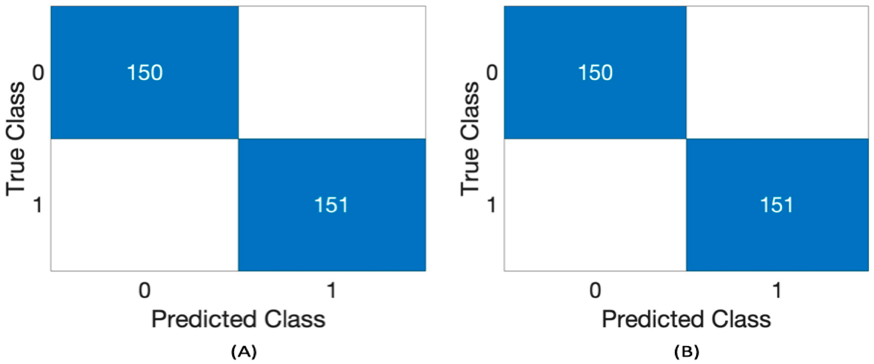
5 s	RF	1.000	1.000	1.000	1.000	1.000	1.000	1.000	1.000	1.000	1.000

presents the performance of the RF classifier using the Challenge 2016 dataset across different segment lengths: 1, 3, and 5 s and two feature sets, 4 and 8. Five performance metrics were utilized as follows: precision, recall, accuracy, F1 score, and AUC. RF classifier demonstrates good consistency across all metrics for every duration and both feature sets. It achieves perfect scores (1.00) in precision, recall, accuracy, F1 score, and AUC for both the 4 and 8 feature sets across all time intervals (1 s, 3 s, and 5 s). Figure 3 presents the confusion matrix of RF using a 3 s segment length with 4 and 8 features.

Table 4. Classifier’s performance metrics using the test set of the Yaseen2018 dataset.

	Classifier	4 Features					8 Features
Seg.Length		Precision	Recall	Accuracy	F1	AUC	Precision	Recall	Accuracy	F1	AUC
1 s	RF	0.8056	0.7699	0.7920	0.7873	0.8689	0.9231	0.9558	0.9381	0.9391	0.9842
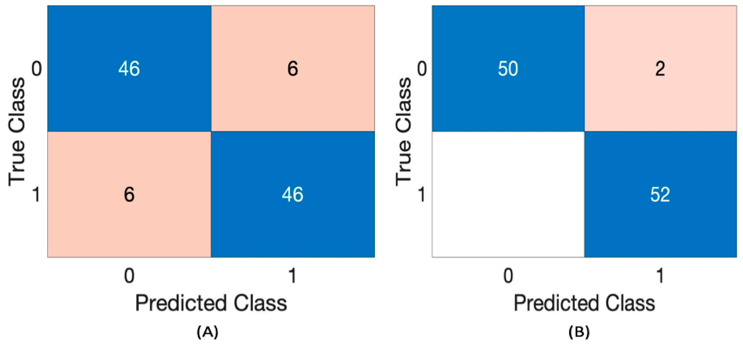
2 s	RF	0.8846	0.8846	0.8846	0.8846	0.9554	0.9630	1.000	0.9808	0.9811	0.9941

shows the performance of the RF classifier, using the Yaseen2018 dataset with a segment length of 1 and 2 s. The evaluated metrics include precision, recall, accuracy, F1 score, and AUC (Area Under the Curve) for the classifier using two feature sets: 4 features and 8 features.

The classifier’s performance using a 1 s segment length with 4 features achieves a precision of approximately 80%, recall of 77%, accuracy and F1 score around 78%, and an AUC of 87%. However, when using 8 features with the same segment length, the classifier demonstrates notable improvements across all metrics. It achieves a precision of 92.3%, recall of 95.6%, accuracy of 93.8%, F1 score of 93.9%, and an AUC of 98.4%. With a 2 s segment length and 4 features, the classifier maintains strong performance, achieving an F1 score of 88.5%, along with high precision, recall, and accuracy. Increasing to 8 features further enhances performance, yielding 96.30% precision, 1.000 recall, 98.08% accuracy, 98.11% F1 score, and 99.41% AUC. Figure 4 presents the confusion matrix of the RF classifier for the 2 s segment length with 4 and 8 features. Figure 4 presents the confusion matrix of RF using a 2 s segment length with 4 and 8 features.

Table 5. Comparison with published work.

Ref	Year	Train/Valid./Test	Method	SPE/PRE	Recall	Accuracy	F1	AUC
[24]	2020	80/0/20	AEN	99.10%	99.7%	99.8%	99.40%	-
[25]	2020	80/0/20	Autoregressive net	98%	100%	99%	99%	-
[26]	2023	70/15/15	1D CNN	97.7%	87.6%	95.5%	92.7%	-
[27]	2024	80/10/10	ResNet50	98.99%	93.53%	97.87%	97.86%	96.26%
Proposed method Challenge 2016		Train/Test	CSP + RF	100%	100%	100%	100%	100%
Yaseen2018		70/0/30	CSP (8 features) + RF	96.30%	100%	98.08%	98.11%	99.41%

presents the performance results of the state-of-the-art binary heart disease classification methods using the Challenge 2016 dataset in comparison to the approach proposed in this paper.

In Deperlioglu et al. [24], they introduced the binary classification of heart sound using Autoencoder Neural Networks (AEN). Their approach achieved an accuracy of 99.8%, a sensitivity of 99.7%, and a specificity of 99.1% for the PhysioNet/CinC Challenge 2016 dataset. Khaled et al. [25] used a dynamic recurrent network called the non-linear autoregressive network with exogenous inputs (NARX) for the binary classification of heart sound signals. They obtained an accuracy of 99%, a sensitivity of 100%, and a specificity of 98% using the PhysioNet dataset. Hussain et al. [26] investigated the binary classification using one of the recent techniques introduced in deep learning algorithms for audio classification, which is 1-Dimensional Convolutional Neural Network (1D-CNN). Their method achieved an accuracy, sensitivity, specificity, F1 score, and precision of 95.45%, 97.44%, 93.6%, 95.45%, and 95.54%, respectively, with the PhysioNet/CinC Challenge 2016 dataset. Hu et al. [27] introduced an approach for classifying cardiac audio signals by converting the raw cardiac audio signals into multidimensional feature representations, capturing various temporal and frequency-domain characteristics. These features are then expressed as images, enabling the use of deep networks such as ResNet50 to analyze and classify the heart sounds effectively. Their approach achieved an accuracy, sensitivity, specificity, AUC, and F1 score of 97.87%, 93.53%, 98.99%, 96.26%, and 97.86%, respectively, with the PhysioNet/CinC Challenge 2016 dataset.

While our methodology demonstrates robust binary classification efficacy for PCG signals utilizing CSP and RF, specific limitations require attention. The framework presently supports only binary tasks, and extending it to multi-class scenarios would require more advanced feature engineering. CSP depends on variance-based discriminative features, potentially neglecting complex patterns in non-stationary or noisy PCG data. Furthermore, although the model was evaluated using the Challenge2016 and Yaseen2018 datasets, extensive validation across a larger and wider array of real-world recordings is essential to verify its generalizability.

Future work will focus on expanding the approach to multi-class classification by incorporating sophisticated signal representations (such as features derived from deep learning) in order to increase robustness. Additionally, we intend to assess the generalizability of the proposed method on a larger dataset and evaluate its practicality for real-time applications in clinical environments.

5. Conclusions

This study demonstrates that combining CSP feature extraction with the RF classifier offers a highly effective approach for distinguishing between normal and pathological heart sounds. The proposed method achieved outstanding results on both the PhysioNet/CinC Challenge 2016 and Yaseen2018 datasets, indicating its potential as a robust tool for automated cardiac diagnosis. With accuracy, precision, and recall metrics nearing perfection, especially on the PhysioNet dataset, this method could significantly enhance the reliability of heart sound analysis beyond traditional auscultation techniques that rely on clinician expertise. We are planning to expand on these findings by exploring real-time implementations and testing the approach on a larger dataset.