Probabilistic Characterization and Machine Learning-Based Modeling of Conducted Emissions of Programmable Microcontrollers

Abstract

To evaluate the system-level electromagnetic emissions of an automobile, in a simulation environment, individual sources of electromagnetic interference (EMI) must be modeled. Modeling the emission behavior of electronic controller units (ECUs) in automobiles requires the characterization of the main microcontroller as an emission source. The conducted emissions (CEs) of the microcontroller depend on the programs running inside the core and the functional blocks utilized for those programs. We propose a measurement-based stochastic model to characterize such program dependency on the conducted emissions of a microcontroller. From board-level CE measurements and the functional blocks utilized for the programs, we obtain the upper and lower bounds of the emissions within which the microcontroller’s conducted emissions are expected to lie with a 95% confidence interval. Further, we propose a method to estimate the emission peaks of the microcontroller when a new program runs in its core with a ±4 dB average error. The functional blocks used for this analysis involve the RAM, timers, and GPIOs. The method works satisfactorily at frequencies up to 500 MHz and is tested on an STM32 general-purpose microcontroller board.

1. Introduction

The increasing density of electronic components inside modern-day automobiles has led to a significant increase in electromagnetic interference (EMI) issues. A typical electric vehicle consists of various power converters, such as inverters and DC–DC converters, along with some domain-specific electronic control units (ECUs) that contain programmable microcontrollers. These devices involve the switching actions of transistors, which result in current and voltage spikes. Spikes in current and voltage (${\displaystyle \frac{di}{dt}}$ and ${\displaystyle \frac{du}{dt}}$) lead to the generation of EMI, affecting nearby components and potentially leading to system failures. The generation of EMI also results in failures during electromagnetic compatibility (EMC) testing, which is necessary for obtaining vehicle certification and type approvals. To address EMI effectively, early identification through simulation-based modeling is crucial. Modeling the electromagnetic interference phenomenon involves modeling the sources, the coupling paths, and the victims [1]. The switching activity of sources such as power converters is modeled deterministically in [2,3] using tools such as SPICE circuits, while the modeling of programmable components like microcontrollers [4] and FPGAs [5] is far more complex. For the operation of a microcontroller that involves the switching of millions of transistors, a circuit-level simulation is infeasible. Further, the emission signatures of these devices vary with the operating conditions or programs running inside the core. The resulting current peaks, which depend on the number and activity of transistors, as well as the functional blocks used by these devices, act as sources of EMI.

For a single operating condition, due to a specific program running in the microcontroller’s core, the source model is developed deterministically. The ICEM-CE standard [6] models the conducted emission (CE) of integrated circuits (ICs) using an equivalent current source for internal activity (IA), in parallel with the impedance as a passive distribution network (PDN) to be plugged into the simulation environment. In [7,8], the PDN of a 16-bit and a 32-bit microcontroller is modeled using specialized boards that contain just the IC and SMA connectors. The current source is modeled separately for programs involving the RAM, flash memory, PLL circuits, or port operations up to 1 GHz. The current consumption is obtained from historical studies on a similar 16-bit microcontroller and later tuned to match the conducted emission measurement accurately. In [9,10], voltage measurements and PDN impedance measurements at microcontroller pins are used to extract an IC model by solving circuit equations effectively up to 500 MHz [9] and 120 MHz [10]. The accuracy of these methods depends on the precision voltage and PDN measurements. To reduce the dependence on measurement accuracy for IA calculation and fast estimations, ref. [11] proposes a method that uses dynamic power consumption and the switching times provided by IC manufacturers. Another example of obtaining IA without relying on accurate voltage measurements at the pins is presented in [12], where a parameterized IA model is developed using prior information from the microcontroller supplier. The model assumes a triangular pulse shape, calculates its fast Fourier transform, and fine-tunes it to match the known conducted emission behavior. These methods provide a deterministic approach for characterizing microcontroller emissions under a specific operating condition.

However, different operating conditions of a microcontroller lead to different emission behaviors since the emissions depend upon the program running in its core. This behavior is observed in both conducted [13] and radiated emissions [14]. In [15], variations in a microcontroller radiated emission spectrum are observed between 300 MHz and 1 GHz when different instruction sets, such as ADD, MOV, and WAIT, run in the core. Below 70 MHz, the clock source is identified as the primary contributor to the emission spectrum. To fully characterize microcontroller emissions using instruction sets, thousands of programs may be needed [16]. In [17], the radiated emission behavior of a microcontroller is analyzed by correlating its time-varying radiation impedance with the instruction sets in its core through statistical clustering. This method groups arithmetic operations such as ADD, SUB, and DEC into a single cluster; logical and movement operations into other clusters; and jump operations into separate clusters. The program dependence of the microcontroller emissions and the statistical clustering of emissions based on programs are explained in the literature; however, models to predict or estimate the emissions of a microcontroller due to a specific program/instruction(s) are needed.

In [18], time-domain waveforms resulting from different instruction sets are recorded. For a program that contains a combination of these instruction sets, the conducted emissions are estimated by combining the emissions of individual instruction sets in the time domain. In the methodology suggested in [19], a similar approach is extended to a simple operating system, where multiple instruction-specific current source models are created for individual instruction sets in the time domain. For a new program, individual instruction current models are combined to obtain the resultant current waveform. These existing methods use instruction set-based assembly-level programming to model microcontroller emissions. Another approach for modeling IC emissions is proposed by Sicard [20]: a tool based on an empirical method to compute the conducted emissions as a function of the IC technology used, the number of gates switching due to the internal activity of the IC, etc. To utilize these models, exact information on the ICs is needed, which is seldom available outside IC manufacturers.

For a system integrator such as an automobile or an ECU supplier, specialized IC boards designed for EMC-related measurements or information on internal IC properties for die/packages is unavailable. When evaluating the conducted emission of an ECU, with multiple components such as a microcontroller and power converters, transistor-level detailed simulations become computationally large and prohibitive for practical purposes. Since ECUs are programmed with high-level language for performing functional tasks, we need to model the dependence of the conducted emissions on the higher-level program configurations instead of the instruction-level programs. Given these constraints, we aim to characterize the conducted emissions of a microcontroller using a measurement-based stochastic model based on high-level program configurations. For an EMC engineer, focusing solely on the worst-case emission scenarios of a switching device is neither practical nor efficient, as such scenarios occur infrequently. Addressing them exclusively may lead to the design of oversized components for filters chosen for the most extreme cases. A more effective approach is to identify the more probable emission spectrum generated by the microcontroller, enabling optimized design solutions. Furthermore, with advancements in Over-The-Air (OTA) software update technologies, the prediction of emission peaks becomes essential when a new program is executed on the microcontroller core in order to validate its compliance with standard limits. To address these challenges, we propose the following research objectives:

• To obtain the upper and lower bounds within which microcontroller emissions are expected to fall with 95% confidence.
• To accurately obtain the emission peaks of a new program based on the emissions of a set of known programs.

In our previous work [21], we modeled the conducted emissions of an STM32 general-purpose microcontroller as a function of the percentage of RAM utilization by the program running in its core, considering a fixed clock frequency. The research objectives mentioned above were addressed by employing a linear decomposition of the emission space and correlating the principal component coefficients with the RAM utilization. In this paper, this approach is further extended by incorporating more program configurations, such as variable clock frequencies, PLL circuit status (enabled/disabled), and the switching of general-purpose input/output (GPIO) port pins using different timer settings. The methodology developed previously in [21] was tailored for programs with a single clock frequency and variable RAM utilization. However, extending this approach to scenarios with varying clock frequencies requires the clustering of programs with the same clock frequency. Additionally, the previous approach does not account for the effects of GPIO switching, necessitating the development of a new methodology to accommodate such cases. For the first research objective, objective 1, we use a statistical approach to estimate the upper and lower bounds of the conducted emissions of an STM32 microcontroller, which assumes the probability distribution function for the emission envelopes across various configurations. We compute these bounds for a 95% confidence interval. These bounds can further be used to select filter design components without requiring an analysis of the emissions of individual programs. The method also specifies the program combinations that are used to accurately establish these bounds.

To estimate the conducted emissions of a new program running in the core, as outlined in research objective 2, we use a machine learning approach. Traditional first-principle models have inherent limitations in accurately modeling complex phenomena, while machine learning models chosen to capture complex patterns often lack interpretability and the consideration of physical constraints. To bridge this gap, the recent literature proposes frameworks such as the mixture of experts [22], Gaussian mixture models (GMMs) [23,24], and conditional mixture models [25,26], which combine the interpretability of gray-box models with the accuracy of black-box approaches. In this work, we employ the machine learning-based conditional mixture model with linear regression to cluster the conducted emission peaks of various programs and probabilistically predict the emissions of new programs. While the conditional mixture model with linear regression is a well-established technique, its application to conducted emissions prediction is novel. For an STM32 microcontroller, the model performs well, with an average prediction error of ±4dB, and it also explains the statistical similarities between different program types and their emission peaks.

In a real vehicle environment, microcontroller emissions are influenced by interactions with power converters, communication networks, and system-level coupling with wiring harnesses and the metal chassis. We adopt a systematic approach based on the Electronic Board Emission Model (EBEM) [27] to analyze these effects. This involves de-embedding the test fixture effects to derive an equivalent source model of the microcontroller board as a function of the program running in its core. Such models for individual noise sources, along with coupling paths such as wiring harnesses, can be simulated using an electromagnetic solver to assess overall electromagnetic interactions within the vehicle. The present work serves as a precursor to developing equivalent microcontroller source models for integration into realistic electromagnetic environments.

This paper is organized as follows: Section 2 outlines the design of experiments for testing various program configurations of the microcontroller for conducted emissions. Section 3 describes the conducted emission measurement setup. Section 4 introduces the methodology for determining the emission bounds, as described in Section 4.1, and for predicting the emissions of new programs using conditional mixture models, as detailed in Section 4.2. The application of these methods to STM32 microcontroller emissions and the results are discussed in Section 5, and concluding remarks, along with future work, are provided in Section 6.

2. Design of Experiments

An STM32 microcontroller [28] is used as a device under test (DUT), and it consists of a 32-bit ARM Cortex-M0 Central Processing Unit (CPU). Its architectural layout is illustrated in Figure 1. The controller operates with a High-Speed Internal (HSI) clock, with frequencies of 8 MHz and 48 MHz, supplemented by a phase-locked loop (PLL) circuit multiplying the frequencies up to a maximum frequency of 48 MHz. The microcontroller has 16 kB of RAM and 128 kB of flash memory. It consists of 8 timers and supports various communication interfaces such as a Controller Area Network (CAN) and a Serial Peripheral Interface (SPI), an Inter-Integrated Circuit (${\mathrm{I}}^2$C), and a Universal Synchronous/Asynchronous Receiver/Transmitter (USART). The general-purpose input/output (GPIO) pins can be configured using these timers for pulse-width modulation (PWM) signal generation.

The primary noise sources in a microcontroller include oscillator or clock sources, system clock circuits (such as PLLs), output transitions from GPIO switching or communication lines, power supply fluctuations due to transistor switching, and signal transitions on data or address buses. In this work, we focus on the RAM, GPIO, clock control, and timer blocks, shown in Figure 1, as a case study. A RAM-based program exchanges data with the CPU over the Advanced High-Performance Bus (AHB), which derives its clock from the system clock. GPIO operations also utilize the system clock with varying switching frequencies and duty cycles. While ADC and DAC modules introduce power supply fluctuations and rely on the clocking circuit, their functional behavior has similarities to RAM-based programs in terms of data exchange and clock dependency. Likewise, SPI and ${\mathrm{I}}^2$C communication generate signal transitions on data lines and output pins, similar to GPIO switching. Although other functional blocks may contribute to emissions, this study focuses on program-driven interactions in the selected modules, and the approach is adaptable to additional components as needed.

To quantify the activity of the microcontroller core, we run two types of programs:

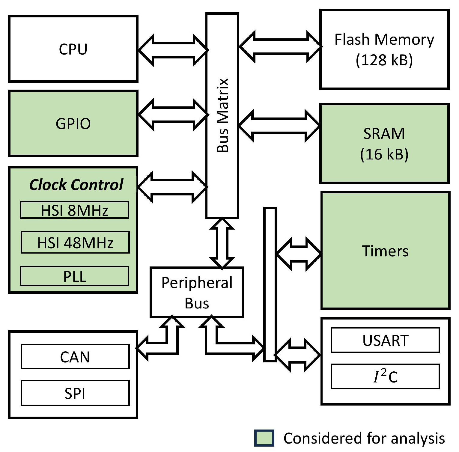
• To evaluate the impact of RAM utilization on conducted emissions, we execute programs that utilize RAM exclusively, without any I/O port operations or communications, while varying the clock frequency and PLL utilization.
• To capture the effect of GPIO switching caused by timer programs, communication processes, or other similar activities, we conduct GPIO pin switching experiments using different configurations while keeping RAM utilization nearly the same.

To vary the percentage of RAM utilization ($R\%$), we run a matrix multiplication program with matrices of varying sizes, such as $A_{3\times 3}\times A_{3\times 3}$ or $A_{35\times 35}\times A_{35\times 35}$, and we obtain the RAM usage from a total of 16 kB. These experiments are carried out with different HSI clock frequencies—8 MHz and 48 MHz—and different combinations of PLL multiplier frequencies, such as $8\times 2=16\mathrm{MHz}$ and $8\times 3=24\mathrm{MHz}$. For each clock (CLK) and PLL configuration, the RAM utilization is systematically varied from 10% to 100%, resulting in a total of 49 experiments. All the combinations of RAM usage, HSI clocks, and PLL multipliers are summarized in

Table 1. Design of experiment—RAM programs.

System Clock (MHz)	PLL Status	${\mathit{A}}_{3\times 3}$ (R%)	${\mathit{A}}_{9\times 9}$ (R%)	${\mathit{A}}_{18\times 18}$ (R%)	${\mathit{A}}_{25\times 25}$ (R%)	${\mathit{A}}_{30\times 30}$ (R%)	${\mathit{A}}_{32\times 32}$ (R%)	${\mathit{A}}_{35\times 35}$ (R%)
8	OFF	10	15	33	55	75	85	100
16	ON	10	15	33	55	75	85	100
24	ON	10	15	33	55	75	85	100
32	ON	10	15	33	55	75	85	100
40	ON	10	15	33	55	75	85	100
48	ON	10	15	33	55	75	85	100
48	OFF	10	15	33	55	75	85	100

.

To perform GPIO switching, we activate various combinations of timers on the STM32 board—TIM1 (4 channels), TIM2 (4 channels), TIM3 (4 channels), TIM14 (1 channel), TIM15 (2 channels), TIM16 (1 channel), and TIM17 (1 channel)—providing a total of 17 channels or pins. These timers generate pulse-width-modulated (PWM) signals with different switching frequencies and duty ratios. For this experiment, the HSI clock is set to 48 MHz with the PLL disabled, and the timer pre-scaler is set to 1.

The switching frequency is changed using an auto-reload value, which specifies the maximum count of the timer before it completes a cycle and resets. With this value, the clock frequency is divided to calculate the switching frequency, $f_s$, as follows:

$$f_s={\displaystyle \frac{f_{clock}}{\mathrm{Auto}\text{-}\mathrm{Reload}\text{-}\mathrm{Value}}}$$

(1)

Further, the duty ratio of the PWM signal is controlled using the capture/compare register (CCR) value, which specifies the fraction of the total period for which the pin voltage is high. The duty ratio (D) can be expressed in terms of the CCR value and the auto-reload value as follows:

$$D={\displaystyle \frac{CCR}{\mathrm{Auto}\text{-}\mathrm{Reload}\text{-}\mathrm{Value}}}$$

(2)

Table 2. Design of experiment GPIO programs—variable frequency.

Auto-Reload Value	Timer Frequency (MHz)	Total Pins	RAM Utilization (R%)
48	1	6	10.5
48	1	12	11
48	1	17	12.75
24	2	6	10.5
24	2	12	11
24	2	17	12.75
12	4	6	10.5
12	4	12	11
12	4	17	12.75

and

Table 3. Design of experiment GPIO programs—variable duty ratio.

Auto-Reload Value	CCR	Duty Ratio (%)	Total Pins	RAM Utilization (R%)
48	5	10	6	10.55
48	5	10	12	11
48	5	10	17	12.75
48	24	50	6	10.55
48	24	50	12	11
48	24	50	17	12.75
48	38	80	6	10.55
48	38	80	12	11
48	38	80	17	12.75

present the program configurations used for switching the GPIO pins with varying frequencies and duty ratios, respectively. In Table 2, the duty ratio is maintained constant at 80%, while the switching frequency varies according to Equation (1). For further analysis and model building, the emission data are sampled at 1 MHz; hence, the switching frequencies ($f_s$) are set to 1 MHz, 2 MHz, and 4 MHz. TIM1 and TIM15 excite a total of six pins; TIM1, TIM2, and TIM3 excite twelve pins; and when all timers are active, seventeen pins are switched. During these experiments, the flash memory utilization is maintained constant at 7–8%.

In Table 3, the clock frequency is set to 48 MHz, with an auto-reload value of 48, resulting in a fixed switching frequency of 1 MHz. The duty ratio is varied in steps of 10%, 50%, and 80%, as calculated using Equation (2). These variations are tested across different timer configurations and numbers of pins.

Together, Table 2 and Table 3 describe 18 GPIO switching experiments. Combined with the RAM utilization experiments, a total of 67 experiments are conducted involving both RAM and GPIO switching programs.

3. Measurement Setup

The conducted emission measurement setup comprised the STM32 microcontroller board as the device under test (DUT), powered by a constant 5 V DC supply from a Rigol DP832 programmable DC power supply. Power and ground pins were connected to two Line Impedance Stabilization Networks (LISNs) from Scientific. The conducted emissions were measured at the LISN connected to the power supply line and observed using a Rohde & Schwarz FPC1000 spectrum analyzer (Model: 102718/002), functioning as an EMI receiver. The ground pin of the DUT was connected to the LISN, while the LISN’s output port was terminated with a 50 Ω impedance. The setup followed the CISPR 25 standard [29], with some modifications. As per the standard, the cable between the DUT and LISN was 20 cm in length, and the DUT was positioned 5 cm above a grounded metal table using a Styrofoam sheet for insulation. The measurements were performed in a closed, unshielded room. However, the measurement table was properly grounded to minimize interference and ensure measurement consistency.

A logarithmic frequency sweep was performed using the spectrum analyzer from 1 MHz to 500 MHz. The resolution bandwidth (RBW) was set to 1 kHz to accurately capture small emission peaks, and the total sweep duration was approximately 111.1 s. Our analysis of the STM32 microcontroller showed no significant emissions above 500 MHz, which is why this frequency was chosen as the upper limit for this study. The complete laboratory setup is shown in Figure 2.

Figure 3 and Figure 4 show examples of the conducted emissions. Since the STM32 board’s main microcontroller is the only switching source on the board, the emission signatures observed on the spectrum analyzer originate solely from the microcontroller IC. Figure 3 displays the emission spectrum from a $9\times 9$ matrix multiplication with an 8 MHz clock frequency, zoomed in between 7 MHz and 500 MHz. The spectrum shows peaks at the 8 MHz clock frequency and its harmonics, as RAM operation occurs at the system clock frequency. Some harmonics fall below the noise floor and are not visible—such small and insignificant peaks are ignored in further analysis.

Similarly, Figure 4 shows the emission spectrum due to the GPIO switching program. In this program, GPIO switching occurs at a 1 MHz frequency for a PWM signal of 80% duty ratio on 12 pins of the microcontroller. In this figure, the emission spectrum is observed from 7 MHz to 500 MHz. It shows peaks at the harmonics of 1 MHz due to GPIO switching, along with peaks corresponding to the clock frequencies at 8 MHz.

4. Methodology

4.1. Estimation of Emission Bounds

In this section, we propose a method to determine the upper and lower emission bounds (in dB$\mathsf{\mu }$V) that define a 95% confidence interval for emission signatures across the given set of measurements. For example, using the measurements from Section 2, this method can identify the confidence bounds for emissions as a function of frequency for the STM32 microcontroller board. For this analysis, we sample the emission spectrum at 1 MHz intervals, extract the emission peaks, and create emission envelopes by interpolating between these peaks over a frequency range of 1–500 MHz. These envelopes are then used for the calculation of the bounds.

In calculating the bounds, we first determine which programs should be considered and how many of them are required. This is achieved by conducting a principal component analysis [30] to identify the programs that primarily influence the variance in emissions. Based on such programs, we create combinations of emission envelopes from the experiments performed in Section 2 and compute the bounds. Combinations that conform to the 95% confidence interval are considered good samples for computing the emission bounds for the microcontroller. This means that the test signal remains within the bounds 95% of the time.

To identify the programs that contribute most to the variance in emissions, let Y be a matrix representing the emission envelope such that $\mathbf{Y}\in {\mathbb{R}}^{M\times N}$, where M is the number of frequency points, and N is the number of programs. The mean of the emissions due to all N programs at any frequency point m is

$${\overline{y}}_m={\displaystyle \frac{1}{N}}\sum _{n=1}^N{\mathbf{Y}}_{mn}\in {\mathbb{R}}^M$$

(3)

Let $\overline{\mathbf{Y}}$ be a mean-centered matrix, where each element is defined as ${\overline{y}}_{mn}=y_{mn}-{\overline{y}}_m$. The covariance matrix R of Y is given by

$$\mathbf{R}={\displaystyle \frac{1}{N}}(\overline{\mathbf{Y}}·{\overline{\mathbf{Y}}}^T)\in {\mathbb{R}}^{M\times M}$$

(4)

Applying Singular Value Decomposition (SVD) [30], a technique used to decompose a matrix into its singular values and vectors, we diagonalize the covariance matrix $\mathbf{R}$, which is a positive semi-definite matrix such that

$$\mathbf{R}=\mathbf{U}·\mathbf{\Sigma }·{\mathbf{U}}^T$$

(5)

where $\mathbf{U}\in {\mathbb{R}}^{M\times M}$ is a matrix containing eigenvectors, and $\mathbf{\Sigma }\in {\mathbb{R}}^{M\times M}$ contains the eigenvalues $\lambda$ of the matrix R arranged in descending order of their magnitude. We select the most significant k eigenvectors corresponding to the first k largest eigenvalues, referred to as the principal components P, such that

$${\mathbf{P}}_k=[\mathbf{U}:\lambda >=1]\in {\mathbb{R}}^M$$

(6)

In Figure 5, from the emission envelopes measured for STM32, we select the first four most significant principal components, ${\mathbf{P}}_{1:4}$, as they collectively explain 85% of the variance in the dataset. The programs are sequentially indexed along the X-axis (Program 1 to Program 67), with the Y-axis displaying the corresponding principal component coefficients. The first 49 programs correspond to RAM utilization (Table 1), while the remaining 18 involve GPIO switching (Table 2 and Table 3). The principal component coefficients show minimal variation for the RAM programs, whereas significant variation is observed for the GPIO programs. To compute the upper and lower bounds of the emissions, we use emission envelopes from both the RAM utilization and GPIO switching programs. To better capture the larger variation in the GPIO programs, the combination includes a higher proportion of them.

The selection of combinations of programs to compute the emission bounds is carried out as follows: ${\mathbf{Y}}_{(1:r)}$ are the first r programs that involve the activity of RAM, and ${\mathbf{Y}}_{(N-g+1):N}$, which are GPIO-based programs, are the last g programs out of all N programs such that $r+g=N$. Out of these programs, we choose the k RAM programs and q GPIO programs such that $k\le q$. To sample optimum combinations of k and q out of r and g, we use Latin Hypercube-based sampling, a statistical method used for generating sample sets that ensure a representative coverage of the input space, and we sample 100 such combinations [31]. Let us choose a matrix A:

$${\mathbf{A}}_{M\times k}=\{{\mathbf{Y}}_{(:,i_1)},{\mathbf{Y}}_{(:,i_2)},...,{\mathbf{Y}}_{(:,i_k)}\}$$

(7)

such that $\{i_1,i_2,...,i_k\}\subseteq \{1,2,...,r\}$, which represents k vectors chosen from the first r emission vectors of the RAM programs. Similarly, we choose matrix B:

$${\mathbf{B}}_{M\times q}=\{{\mathbf{Y}}_{(:,j_1)},{\mathbf{Y}}_{(:,j_2)},...,{\mathbf{Y}}_{(:,j_q)}\}$$

(8)

such that $\{j_1,j_2,...,j_q\}\subseteq \{N-g+1,N-g+2,...N\}$, which represents the q GPIO emission vectors chosen from the last g vectors. Additionally, the matrices $\mathbf{A}M\times k$ and $\mathbf{B}M\times q$ are concatenated to form the envelope matrix $\mathbf{Z}$, where $\mathbf{Z}\in {\mathbb{R}}^{M\times (k+q)}$. The mean ($\mu$) and standard deviation ($\sigma$) are computed for every row of $\mathbf{Z}$ for each frequency point as follows:

$$\mathbf{Z}={\left[\mathbf{A}\right|\mathbf{B}]}_{M\times (k+q)}$$

(9)

$${\mu }_m={\displaystyle \frac{1}{k+q}}\sum _{j=1}^{k+q}{\mathbf{Z}}_{mj}\mathrm{for}m=1,...,M$$

(10)

$${\sigma }_m=\sqrt{{\displaystyle \frac{1}{k+q}}\sum _{j=1}^{k+q}{({\mathbf{Z}}_{mj}-{\mu }_m)}^2}\mathrm{for}m=1,...,M$$

(11)

For the calculation of the emission bounds, we assume the combination of emissions to be distributed using Student’s t-distribution [32], which is a suitable assumption for small-sized samples. For Student’s t-distribution, for every frequency point in Z, characterized by certain degrees of freedom and confidence intervals, the upper bound (${\mathbf{l}}_u$) and lower bound (${\mathbf{l}}_l$) within which the emissions will lie are defined such that

$${\mathbf{l}}_u={[{\mu }_m+t_{\alpha /2}·\sqrt{1+1/n}·{\sigma }_m]}_{m=1}^M$$

(12)

$${\mathbf{l}}_l={[{\mu }_m-t_{\alpha /2}·\sqrt{1+1/n}·{\sigma }_m]}_{m=1}^M$$

(13)

where $t_{\alpha /2}$ is the t-value with (n − 1) degrees of freedom and a (1 $- \alpha$) confidence level. To validate the emission band computation, a test signal is chosen: ${\mathbf{z}}_{test}={\mathbf{Y}}_{(:,j)}$, where j is chosen at random from $\{1,2,..(k+q\left)\right\}$. ${\mathbf{z}}_{test}$ is omitted from Y while computing ${\mathbf{l}}_l$ and ${\mathbf{l}}_u$. Later, ${\mathbf{z}}_{test}$ is compared with ${\mathbf{l}}_l$ and ${\mathbf{l}}_u$ to check the following:

$$\mathbb{P}({\mathbf{l}}_l<{\mathbf{z}}_{\mathrm{test}}<{\mathbf{l}}_u)=0.95$$

(14)

All RAM and GPIO program combinations $(k,q)$ that satisfy Equation (14) from the matrix $\mathbf{Z}$ are considered good samples to estimate the upper and lower bounds. Further, the ${\mathbf{l}}_u$ and ${\mathbf{l}}_l$ of these samples represent the upper and lower emission bounds with 95% confidence for the microcontroller.

4.2. Prediction of Emissions of a New Program

In the following section, we propose a methodology for predicting the emission peaks due to a new program running in the core of the microcontroller in the 1-500 MHz frequency range, which is characterized by different program configurations. Based on the design of experiments presented in Section 2, we aim to characterize the emission peaks based on the following program configurations: the RAM percentage utilization ($R\%$), clock frequency, PLL status (on/off), switching frequency ($f_s$) of the GPIO pins, duty ratio for switching the GPIO pins, and number of pins switching during the program’s runtime. Let X be the input matrix, defined as [${\mathbf{x}}_{\mathbf{1}},{\mathbf{x}}_{\mathbf{2}},...,{\mathbf{x}}_{\mathbf{p}}$], where ${\mathbf{x}}_i$ is the program configuration called the parameter such that $\mathbf{X}\in {\mathbb{R}}^{P\times N}$, where N is the number of programs, and P is the number of parameters. Let y be the output vector that contains the emission peaks of each program at a single frequency point. A generalized regression model is of the form

$$\mathbf{y}={\mathbf{w}}^{\top }\varphi +ϵ$$

(15)

where $\varphi$ represents the basis function in X, and $\mathbf{w}$ is a weight matrix such that $\mathbf{w}\in {\mathbb{R}}^P$. In our previous work [21], we modeled $\varphi$ as a function that decomposes the emissions y into basis vectors, with the weights $\mathbf{w}$ assumed to be proportional to the percentage of RAM utilization, provided that all programs operated at a fixed clock frequency. When extending this approach to accommodate multiple program configurations, X must be clustered into groups with a constant clock frequency and variable RAM utilization. Basis vectors should be derived for each group, and y is estimated accordingly. In each case, the relationship between the weights $\mathbf{w}$ and RAM utilization percentage must be determined. For programs involving GPIO switching, there is no straightforward or sophisticated method for grouping the programs. Consequently, the approach used for RAM-based programs may not directly apply to GPIO switching programs. These challenges in extending the previously developed method necessitate the development of a new algorithm with the following requirements:

• Statistically cluster X into distinct groups and justify the assignment of input data to specific clusters.
• Determine the weights associated with each cluster.
• Estimate emissions through a regression model.

To address these requirements, we propose using a conditional mixture model [26], which is well suited for modeling emission peaks due to its properties as follows: This model determines the probability with which each data point (i.e., program emission peak) belongs to a particular cluster and simultaneously learns the weights and mixing coefficients that conditionally combine the contributions from relevant clusters. Since the selection of clusters is driven by input variables, different clusters can be responsible for making predictions in distinct regions of the input space. In this study, we apply a conditional mixture model using linear regression to predict emissions. We define a model for a single frequency point y ($\mathbf{y}\in {\mathbb{R}}^N$) and repeat the procedure for all M frequency points. A generalized linear regression model is of the form

$$\mathbf{y}={\mathbf{w}}^{\top }\mathbf{X}+\mathit{ϵ}$$

(16)

where $\mathbf{w}$ is a weight matrix such that $\mathbf{w}\in {\mathbb{R}}^P$. The noise in the measurement is modeled as a Gaussian variable $\mathit{ϵ}$ of the form $\mathit{ϵ}\sim \mathcal{N}(0,{\beta }^{-1}\mathbf{I})$, where ${\beta }^{-1}$ is the variance in noise. Assume that the model has K clusters. Each cluster is modeled using linear regression with weights ${\mathbf{w}}_k$. The mixing coefficient for each cluster is denoted by ${\pi }_k$. The model is required to learn the following parameters:

• The weight matrix $\mathbf{w}$, such that $\mathbf{w}\in {\mathbb{R}}^{P\times K}$.
• The mixing coefficients $\mathbf{\pi }$, such that $\mathbf{\pi }\in {\mathbb{R}}^K$.
• The noise variance ${\beta }^{-1}$ (also called a precision parameter and considered the same for all clusters).

With the above parameters, the likelihood function is written as

$$\mathbf{p}\left(\mathbf{y}\right|\mathit{\theta })=\sum _k{\pi }_k·\mathcal{N}\left(\mathbf{y}\right|{\mathbf{w}}_k^{\top }\mathbf{X},{\beta }^{-1}\mathbf{I})$$

(17)

where $\mathit{\theta }$ contains all the adaptive parameters. $\mathit{\theta }={\{{\pi }_k,{\mathbf{w}}_k,{\beta }^{-1}\mathbf{I}\}}_{k=1}^K$. Further taking logs on both sides,

$$log\mathbf{p}\left(\mathbf{y}\right|\mathit{\theta })=\sum _{n=1}^{N}log\sum _{k=1}^K{\pi }_k·\mathcal{N}\left(y_n\right|{\mathbf{w}}_k^{\top }{\mathbf{X}}_n,{\beta }^{-1}\mathbf{I})$$

(18)

To find the optimal values of the parameters in $\mathit{\theta }$, we use the expectation maximization (EM) algorithm. This algorithm maximizes the log-likelihood function from Equation (18). For the initialization of $\mathit{\theta }$, we assume a uniform distribution for $\mathit{\pi }$ such that program emission peaks belong to each cluster with equal likelihood. Therefore, $\mathit{\pi }=[1/k,1/k,...1/k]$ (K times). The weights, $\mathbf{w}k$, are initialized randomly multiple times, and the weights that lead to the smallest training error are chosen. Furthermore, the precision parameter $\beta$ is initialized to 1.

In the expectation calculation (E) step, the likelihood of every emission peak $y_n$ belonging to a cluster k is given by

$$\mathbf{p}\left(y_n\right|h_k)=\mathcal{N}\left(y_n\right|{\mathbf{w}}_k^{\top }{\mathbf{X}}_n,{\beta }^{-1})$$

(19)

where $h_k$ is the hypothesis that an emission peak, $y_n$, belongs to cluster k. Further, we compute the posterior probability after observing the data using Bayes’ Theorem. Let the posterior probability $\mathbf{p}\left(h_k\right|y_n)={\gamma }_{nk}$ be defined for each program such that $\gamma \in {\mathbb{R}}^{N\times K}$.

$${\gamma }_{nk}={\displaystyle \frac{{\pi }_k·\mathcal{N}\left(y_n\right|{\mathbf{w}}_k^{\top }{\mathbf{X}}_n,{\beta }^{-1})}{{\sum }_{k=1}^K{\pi }_k·\mathcal{N}\left(y_n\right|{\mathbf{w}}_k^{\top }{\mathbf{X}}_n,{\beta }^{-1})}}$$

(20)

For the maximization (M) step, the values of ${\pi }_k$, ${\mathbf{w}}_k$ and $\beta$ are updated using a closed-form solution to the EM algorithm such that the log-likelihood of Equation (18) is maximized [26].

$${\pi }_k={\displaystyle \frac{1}{N}}·\sum _{n=1}^N{\gamma }_{nk}$$

(21)

Let ${\mathbf{R}}_k=\mathrm{diag}\left({\gamma }_{nk}\right)$, defined for each k, such that ${\mathbf{R}}_k\in {\mathbb{R}}^{N\times N}$.

$${\mathbf{w}}_k={({\mathbf{X}}^{\top }·{\mathbf{R}}_k·\mathbf{X})}^{-1}·{\mathbf{X}}^{\top }·{\mathbf{R}}_k·\mathbf{y}$$

(22)

$${\displaystyle \frac{1}{\beta }}={\displaystyle \frac{1}{N}}·\sum _{n=1}^N\sum _{k=1}^K{\gamma }_{nk}·{(y_n-{{\mathbf{w}}_k}^{\top }{\mathbf{X}}_n)}^2.$$

(23)

When the log-likelihood is maximized, the EM algorithm converges.

To estimate the emissions of a new test program $\mathbf{y}test\in R^N$, we use the optimized weights and mixing coefficients obtained from Equations (21)–(23) based on the parameters ${\mathbf{X}}_{test}$. The predicted outcomes ${\mathbf{w}}_k^{\top }·{\mathbf{X}}_{test}$ are weighted by the mixing coefficients ${\pi }_k$, which are summed to compute the estimated emissions ${\widehat{\mathbf{y}}}_{test}$ as follows:

$${\widehat{\mathbf{y}}}_{test}=\sum _{k=1}^K{\pi }_k·{\mathbf{w}}_k^{\top }·{\mathbf{X}}_{test}$$

(24)

This procedure is repeated over all frequency points M to estimate the emission peaks over the entire frequency spectrum. The metrics chosen to evaluate model performance are the root mean squared error (RMSE) and the $R^2$ score. The root mean squared error is calculated as

$$\mathbf{e}=\sqrt{{\displaystyle \frac{1}{M}}\sum _{i=1}^M{\left(y_{\mathrm{test},i}-{\widehat{y}}_{\mathrm{test},i}\right)}^2}$$

(25)

Further, the $R^2$ score is a measure of variance in the data explained by the model. Let ${\overline{\mathbf{y}}}_{\mathbf{test}}$ be the mean, and let ${\widehat{\mathbf{y}}}_{\mathbf{test}}$ be the estimated value of the test data ${\mathbf{y}}_{\mathbf{test}}$. Then, the $R^2$ score for model testing is given by

$$R_{score,testing}^2=1-{\displaystyle \frac{{\sum }_{N\times M}{\left({\mathbf{y}}_{\mathbf{test}}-{\widehat{\mathbf{y}}}_{\mathbf{test}}\right)}^2}{{\sum }_{N\times M}{\left({\mathbf{y}}_{\mathbf{test}}-{\overline{\mathbf{y}}}_{\mathbf{test}}\right)}^2}}$$

(26)

Determining the Optimal Number of Clusters

In order to maximize the likelihood while avoiding overfitting, the number of clusters should be determined in such a way that balances the fit of the data with the complexity of the model. Increasing the number of clusters improves the likelihood of an emission peak belonging to a cluster while it also increases the complexity of the model. To address this trade-off, we use the Bayesian Information Criterion (BIC) [26], which rewards the increased likelihood and penalizes the model complexity due to the addition in the number of clusters. The overall BIC score, computed with the optimal parameters ${\mathit{\theta }}_{\mathit{opt}}$, is expressed as

$$BI{C}_{\mathrm{score}}=-2log\left[\mathbf{p}\left(\mathbf{y}\right|{\mathit{\theta }}_{\mathrm{opt}})\right]+n·log\left(N\right)$$

(27)

where $log\left[\mathbf{p}\right(\mathbf{y}\left|\mathit{\theta }\mathrm{opt}\right)]$ represents the log-likelihood of an emission peak y belonging to a cluster after the EM algorithm converges with the optimized $\mathit{\theta }\mathit{opt}$, and the term n is the number of parameters in the model for each cluster, while N is the number of data points, i.e., programs. The first term captures the improvement in log-likelihood with additional clusters, while the second term $n·log\left(N\right)$ penalizes the model complexity. Finally, models with different numbers of clusters are compared based on their BIC scores to identify the optimal clustering configuration.

5. Results and Discussion

5.1. Emission Band Estimation

In this section, we present the results of applying the method to the STM32 microcontroller data, generated from the experiments described in Section 2, for the calculation of the emission bounds. The lower and upper bounds (${\mathbf{l}}_l$ and ${\mathbf{l}}_u$) are computed following the methodology outlined in Section 4.1, ensuring that the emissions remain within these bounds with 95% confidence. In Figure 5, it is evident that a higher proportion of GPIO programs should be included in the analysis. To evaluate the methodology, we randomly select a GPIO-based program as a test case (${\mathbf{z}}_{test}$). The combinations of RAM and GPIO programs that satisfy the 95% confidence interval are identified in a comparison with ${\mathbf{z}}_{test}$ using Equation (14). The combinations that meet the criteria of Equation (14) are considered good samples and are plotted in Figure 6.

The region containing the suitable combinations (or good samples) of RAM and GPIO programs, which ensure adherence to the 95% confidence criterion, is highlighted in Figure 6. Any combination within the highlighted area can be used to randomly select the corresponding number of RAM and GPIO programs and compute the emission bounds with 95% confidence. For instance, in Figure 7, the emission bounds are calculated using five RAM and sixteen GPIO programs. The test signal fits well within the computed bounds across the entire frequency range. Based on the upper bound, we infer that the microcontroller’s conducted emissions (CEs) remain at nearly 40 dB$\mathsf{\mu }$V up to 40 MHz, decrease to 30 dB$\mathsf{\mu }$V up to 200 MHz, and further drop to 20 dB$\mathsf{\mu }$V up to 500 MHz, with 95% confidence, for any of the programs described in the design of experiments.

5.2. Conditional Mixture Model for Emission Estimation

This section presents the results of estimating the conducted emission peaks caused by a new program, characterized by specific program configurations, for the STM32 microcontroller across a frequency range of 1–500 MHz. The program configurations include the RAM utilization percentage, clock frequency, PLL status (on/off), GPIO switching frequency, GPIO duty ratio, and number of active GPIO pins, yielding a total of $P=6$ input variables for $N=500$ frequency points. Conditional mixture models are built for each frequency point according to the procedure outlined in Section 4.2. To determine the optimum number of clusters, the model-building process is repeated for different values of K, ranging from 3 to 30 clusters. For each number of clusters, the BIC scores are plotted against the number of clusters for two arbitrarily selected frequency points, 40 MHz and 120 MHz, as shown in Figure 8.

The optimal model is determined by the smallest BIC score, and, based on the observed trend, $K=9$ clusters are selected as the best model. Using $K=9$, a conditional mixture model is created following Equations (17)–(23). The expectation (E) and maximization (M) steps are repeated until the model converges. Upon convergence, the EM algorithm maximizes the log-likelihood. Figure 9 illustrates the log-likelihood observed over eight iterations for three frequency points (8 MHz, 40 MHz, and 120 MHz), showing stabilization at a maximum value, which confirms the model convergence.

For model building and validation, 80% of the total dataset is used for training the model, while the remaining 20% of the data are used for testing the model. The training phase involves estimating the model parameters at each frequency point—${\mathbf{w}}_k$, ${\mathit{\pi }}_k$, and $\beta$—using Equations (19)–(23), as outlined in Section 4.2. Once trained, the emission peaks of the test data are predicted using Equation (24). The performance of the model is evaluated using two key metrics, namely, the 2-norm error and $R^2$ score, computed through Equations (25) and (26). During training, the model achieves a root mean squared error of 3.35 dB$\mathsf{\mu }$V and an $R_2$ score of 0.79, indicating a good fit for the training data. For testing, the root mean squared error increases slightly to 4.45 dB$\mathsf{\mu }$V, with an $R^2$ score of 0.66, reflecting the model’s ability to generalize to unseen data or predict the emission peaks of the configurations of a new program. Figure 10 presents a comparison of the predicted emission peaks and the actual values (in dB$\mathsf{\mu }$V) for both the training and testing datasets, demonstrating the model’s predictive accuracy across the entire frequency range.

The estimated and actual emission peaks of a RAM utilization-based program and a GPIO switching-based program, both from the testing dataset, are presented in Figure 11 and Figure 12. The RAM-based test program is configured with 85% RAM utilization, performing matrix multiplication on $32\times 32$ matrices and operating at a clock frequency of 16 MHz, with the PLL enabled and no GPIO switching. The GPIO switching-based test program features 11% RAM utilization, a clock frequency of 48 MHz without an active PLL, GPIO switching at a frequency of 1 MHz with an 80% duty cycle, and 12 active GPIO pins. For both the program emission peaks, we observe a good match between the prediction and the actual peaks up to 500 MHz.

The conditional mixture model is also used to explain the presence of different clusters in the input space. Figure 13a shows the emission peaks at 8 MHz for various programs in the training dataset. Similarly, Figure 13b plots the likelihood function $\mathbf{p}\left(\mathbf{y}\right|{\mathbf{h}}_{\mathbf{k}})$ against the emission peaks $\mathbf{y}$ in dB$\mathsf{\mu }$V at 8 MHz. Each curve in Figure 13b represents a probability distribution for a different statistical cluster K, which, in reality, may correspond to distinct sets of input variables or program configurations. The training dataset includes a mix of RAM-based and GPIO-based programs. As indicated in Figure 5, RAM-based programs generally produce emission peaks with minimal variation. Changes in clock frequency or enabling the PLL has a smaller influence on emissions. However, GPIO parameters, such as the switching frequency and duty ratio, have a larger effect on emission peaks. In Figure 13a, we observe a cluster of emission peaks around 20 dB, forming a dense data cloud likely attributed to the RAM-based programs. This is reflected in Figure 13b, where four probability curves $\mathbf{p}\left(\mathbf{y}\right|{\mathbf{h}}_{\mathbf{k}})$ are centered around 20 dB with varying standard deviations. In contrast, the emission peaks exceeding 30 dB in Figure 13a exhibit greater scatter, indicating higher variance, likely due to the GPIO-based programs. These higher emission peaks correspond to probability distributions with greater variance, forming five distinct clusters. Each program’s emission can belong to one or more clusters with different probabilities.

6. Conclusions

Microcontroller interactions are inherently complex, involving multiple power domains, power rails, and high-frequency parasitic effects. Various functional blocks contribute to emissions, and electromagnetic coupling between different power paths results in a superposition of noise at the LISN voltage. Developing a deterministic, physics-based model to capture these interactions for different programs is challenging. Therefore, this paper presents a measurement-based stochastic approach to characterize conducted emissions, represented by the LISN voltage of a programmable microcontroller. While several inter-IC interactions influence emissions, certain effects remain consistent for similar programs, and within the same IC, parasitic or power rail interactions exhibit the same behavior. The proposed statistical model captures all such aspects and encodes the effects as statistical features (weights and mixing coefficients) for a program configuration. Consequently, the model parameters derived from these methods are specific to a given board, IC, and frequency.

The proposed methodology is validated using an STM32 microcontroller, covering a broad range of operating conditions. We vary RAM utilization and clock frequencies and enable/disable the phase-locked loop (PLL) circuit. Additionally, we activate I/O ports by inducing the state transitions of pins via timer programs and analyze their impact on the conducted emissions.

To address the characterization of programmable devices in conducted emission tests, we propose a procedure to compute the upper and lower emission bounds with 95% confidence. These bounds are derived from emission envelopes corresponding to various program configurations. Importantly, the methodology identifies the minimal set of 20–25 programs required to compute these bounds for the STM32 device under test, avoiding the need to test thousands of programs to account for all possible emission signatures. Furthermore, we propose a machine learning framework called the conditional mixture model, specifically chosen for the better explainability of new programs with specific configurations. We predict the emission peaks of a new program up to 500 MHz with an RMSE of ±4 dB. Considering that conducted emission measurements of the same device across different labs can vary by 3–5 dB [33], this level of accuracy is highly practical. The proposed model not only provides accurate predictions but also offers statistical insights into the data clusters, which correspond to known program distinctions, such as RAM-based versus GPIO-based programs. This dual capability of prediction and explainability enhances the method’s utility.

Future work will explore additional program parameters beyond those considered in this study. We also aim to validate this approach on a broader range of microcontroller devices, including automotive-grade MCUs and different architectures, to confirm the model’s generalizability and conduct extensive measurements to ensure consistent model performance. While this study focuses on emissions up to 500 MHz, more powerful digital ICs may exhibit significant emission peaks beyond this range under different operating conditions. Notably, the proposed statistical methodology is frequency-independent, allowing for its extension to a broader spectrum in future work. However, accurate techniques must be carefully developed to ensure the reproducibility of conducted emission measurements at higher frequencies (>500 MHz), where radiated emissions become more prominent. The methodology could be applied to characterize the emissions of any device where varying operating conditions influence emissions. While the influencing variables may differ across devices, the approach remains generalizable.

In this study, we focus on characterizing the LISN voltage of a microcontroller PCB based on program configurations. Future work will involve de-embedding the CE test setup, including the cables and LISN, to derive the equivalent board-level source model, the EBEM, between the power and the ground. Modeling an ECU requires an IC-level representation of the microcontroller’s noise source between its power and ground pin(s). To achieve this, we propose further de-embedding of PCB traces to obtain the ICEM-CE source model. This IC-level model can then be integrated into any ECU board where the microcontroller is deployed, capturing program-dependent emissions within a simulation environment. Once the ECU board’s equivalent noise source model is established, it can be combined with electromagnetic models of other electronic boards, such as power converters and communication modules, enabling a comprehensive analysis of the electromagnetic interactions within the vehicle environment.

References

1. Paul, C.R.; Scully, R.C.; Steffka, M.A. Introduction to Electromagnetic Compatibility; John Wiley & Sons: Hoboken, NJ, USA, 2022. [Google Scholar]
2. Kharanaq, F.A.; Emadi, A.; Bilgin, B. Modeling of conducted emissions for EMI analysis of power converters: State-of-the-art review. IEEE Access 2020, 8, 189313–189325. [Google Scholar] [CrossRef]
3. Trinchero, R.; Stievano, I.S.; Canavero, F.G. Enhanced time-invariant linear model for the EMI prediction of switching circuits. IEEE Trans. Electromagn. Compat. 2020, 62, 2294–2302. [Google Scholar] [CrossRef]
4. Stievano, I.S.; Rigazio, L.; Canavero, F.G.; Cunha, T.R.; Pedro, J.C.; Teixeira, H.M.; Girardi, A.; Izzi, R.; Vitale, F. Behavioral modeling of IC memories from measured data. IEEE Trans. Instrum. Meas. 2011, 60, 3471–3479. [Google Scholar] [CrossRef]
5. Ghfiri, C.; Durier, A.; Marot, C.; Boyer, A.; Ben Dhia, S. Modeling the internal activity of an FPGA for conducted emission prediction purpose. In Proceedings of the 2018 IEEE International Symposium on Electromagnetic Compatibility and 2018 IEEE Asia-Pacific Symposium on Electromagnetic Compatibility (EMC/APEMC), Suntec City, Singapore, 14–18 May 2018; pp. 309–314. [Google Scholar]
6. IEC SC47A/WG9; Models of Integrated Circuits for EMI Behavioral Simulation. International Electrotechnical Commission (IEC): Geneva, Switzerland, 1997.
7. Labussière-Dorgan, C.; Bendhia, S.; Sicard, E.; Tao, J.; Quaresma, H.J.; Lochot, C.; Vrignon, B. Modeling the electromagnetic emission of a microcontroller using a single model. IEEE Trans. Electromagn. Compat. 2008, 50, 22–34. [Google Scholar] [CrossRef]
8. Leca, J.P.; Froidevaux, N.; Dupré, P.; Jacquemod, G.; Braquet, H. EMI measurements, modeling, and reduction of 32-Bit high-performance microcontrollers. IEEE Trans. Electromagn. Compat. 2014, 56, 1035–1044. [Google Scholar] [CrossRef]
9. Serpaud, S.; Levant, J.L.; Poiré, Y.; Meyer, M.; Tran, S. ICEM-CE extraction methodology. In Proceedings of the EMC Compo, Toulouse, France, 17–19 November 2009. [Google Scholar]
10. Yuan, S.Y.; Liao, S.S. Automatic conducted-EMI microcontroller model building. In Proceedings of the 2013 9th International Workshop on Electromagnetic Compatibility of Integrated Circuits (EMC Compo), Nara, Japan, 15–18 December 2013; pp. 138–141. [Google Scholar]
11. Ghfiri, C.; Boyer, A.; Durier, A.; Dhia, S.B. A new methodology to build the internal activity block of ICEM-CE for complex integrated circuits. IEEE Trans. Electromagn. Compat. 2017, 60, 1500–1509. [Google Scholar] [CrossRef]
12. Yuanhao, L.; Shuguo, X.; Yishu, C. A new methodology to build the ICEM-CE model for microcontroller units. In Proceedings of the 2021 IEEE International Workshop on Electromagnetics: Applications and Student Innovation Competition (iWEM), Guangzhou, China, 28–30 November 2021; pp. 1–3. [Google Scholar]
13. Ramdani, M.; Sicard, E.; Boyer, A.; Dhia, S.B.; Whalen, J.J.; Hubing, T.H.; Coenen, M.; Wada, O. The electromagnetic compatibility of integrated circuits—Past, present, and future. IEEE Trans. Electromagn. Compat. 2009, 51, 78–100. [Google Scholar] [CrossRef]
14. Baharuddin, M.H.; Islam, M.T.; Yuwono, T.; Smartt, C.J.; Thomas, D.W. Impact of Mode of Operations on the Electromagnetic Emissions of a Complex Electronic Device. In Proceedings of the 2020 IEEE International RF and Microwave Conference (RFM), Kuala Lumpur, Malaysia, 14–16 December 2020; pp. 1–4. [Google Scholar]
15. Fiori, F.; Musolino, F. Analysis of EME produced by a microcontroller operation. In Proceedings of the Design, Automation and Test in Europe, Conference and Exhibition 2001, Munich, Germany, 13–16 March 2001; pp. 341–345. [Google Scholar]
16. Yuan, S.Y.; Tang, Y.C.; Chen, C.C. Software-related EMI test pattern auto-generation for 2-stage pipeline microcontroller. In Proceedings of the 2015 IEEE Symposium on Electromagnetic Compatibility and Signal Integrity, Santa Clara, CA, USA, 15–21 March 2015; pp. 306–309. [Google Scholar]
17. Chen, J.; Portillo, S.; Heileman, G.; Hadi, G.; Bilalic, R.; Martínez-Ramón, M.; Hemmady, S.; Schamiloglu, E. Time-varying radiation impedance of microcontroller GPIO ports and their dependence on software instructions. IEEE Trans. Electromagn. Compat. 2022, 64, 1147–1159. [Google Scholar] [CrossRef]
18. Wada, O.; Saito, Y.; Nomura, K.; Sugimoto, Y.; Matsushima, T. Power supply current analysis of micro-controller with considering the program dependency. In Proceedings of the 2011 8th Workshop on Electromagnetic Compatibility of Integrated Circuits, Dubrovnik, Croatia, 6–9 November 2011; pp. 93–98. [Google Scholar]
19. Yuan, S.Y.; Chung, H.E.; Liao, S.S. A microcontroller instruction set simulator for EMI prediction. IEEE Trans. Electromagn. Compat. 2009, 51, 692–699. [Google Scholar] [CrossRef]
20. Sicard, E.; Bouhouch, L. Using ICEM Model Expert to Predict TC1796 Conducted Emission. Available online: http://www.ic-emc.org/appnotes/Ic-Emc-Application-Note-Tricore-v2.pdf (accessed on 7 April 2025).
21. Gavai, A.; Hansen, J.; Dhoot, V.; Gope, D. Stochastic modeling of microcontroller emission. In Proceedings of the 2023 IEEE 32nd Conference on Electrical Performance of Electronic Packaging and Systems (EPEPS), Milpitas, CA, USA, 15–18 October 2023; pp. 1–3. [Google Scholar]
22. Leoni, J.; Breschi, V.; Formentin, S.; Tanelli, M. Explainable data-driven modeling via mixture of experts: Towards effective blending of gray and black-box models. Automatica 2025, 173, 112066. [Google Scholar] [CrossRef]
23. Mulwa, M.M.; Mwangi, R.W.; Mindila, A. GMM-LIME explainable machine learning model for interpreting sensor-based human gait. Eng. Rep. 2024, 6, e12864. [Google Scholar] [CrossRef]
24. Alangari, N.; Menai, M.E.B.; Mathkour, H.; Almosallam, I. Intrinsically Interpretable Gaussian Mixture Model. Information 2023, 14, 164. [Google Scholar] [CrossRef]
25. Bishop, C.M. Mixture Models and the EM Algorithm; Microsoft Research: Cambridge, UK, 2006. [Google Scholar]
26. Bishop, C.M.; Nasrabadi, N.M. Pattern Recognition and Machine Learning; Springer: Berlin/Heidelberg, Germany, 2006; Volume 4. [Google Scholar]
27. Gavai, A.; Gope, D.; Dhoot, V.; Hansen, J. Electronic Board Emission Model and its Application for Microcontroller Emission. In Proceedings of the 2024 IEEE Joint International Symposium on Electromagnetic Compatibility, Signal & Power Integrity: EMC Japan/Asia-Pacific International Symposium on Electromagnetic Compatibility (EMC Japan/APEMC Okinawa), Okinawa, Japan, 20–24 May 2024; pp. 587–590. [Google Scholar]
28. STMicroelectronics. Arm®-Based 32-Bit MCU, up to 128 KB Flash, Crystal-Less USB FS 2.0, CAN, 12 Timers, ADC, DAC & comm. Interfaces, 2.0–3.6 V. Technical Report, STMicroelectronics, 2019. STM32F072x8/xB Datasheet, Rev 6. Available online: https://www.st.com/resource/en/datasheet/stm32f072c8.pdf (accessed on 7 April 2025).
29. CISPR 25:2021; Vehicles, Boats, and Internal Combustion Engines—Radio Disturbance Characteristics—Limits and Methods of Measurement for the Protection of on-Board Receivers Apparatus. International Electrotechnical Commission (IEC): Geneva, Switzerland, 2021.
30. Lang, S. Introduction to Linear Algebra; Springer: Berlin/Heidelberg, Germany, 2012. [Google Scholar]
31. Dutta, S.; Gandomi, A.H. Design of experiments for uncertainty quantification based on polynomial chaos expansion metamodels. In Handbook of Probabilistic Models; Elsevier: Amsterdam, The Netherlands, 2020; pp. 369–381. [Google Scholar]
32. Walpole, R.E.; Myers, R.H.; Myers, S.L.; Ye, K. Probability and Statistics for Engineers and Scientists; Macmillan: New York, NY, USA, 1993; Volume 5. [Google Scholar]
33. CISPR 16-4-2; Specification for Radio Disturbance and Immunity Measuring Apparatus and Methods—Part 4-2: Uncertainties, Statistics and Limit Modeling—Measurement Instrumentation Uncertainty. International Electrotechnical Commission (IEC): Geneva, Switzerland, 2011.
Figure 1. Functional block representation of micro-controller [28].
Electronics 14 01511 g001
Figure 2. Conducted emission setup with the microcontroller as the DUT.
Electronics 14 01511 g002
Figure 3. Emission spectrum for 9 × 9 matrix multiplication program.
Electronics 14 01511 g003
Figure 4. Emission spectrum for timer program with 1 MHz switching.
Electronics 14 01511 g004
Figure 5. Principal components (PCs) of emission matrix against different programs.
Electronics 14 01511 g005
Figure 6. The green region represents samples that satisfy the criterion of the 95% confidence interval.
Electronics 14 01511 g006
Figure 7. Upper and lower limit bands with test signal peaks from 1 to 500 MHz.
Electronics 14 01511 g007
Figure 8. BIC score against the number of clusters.
Electronics 14 01511 g008
Figure 9. Log-likelihood values over iteration count for frequency points 8 MHz, 40 MHz, and 120 MHz.
Electronics 14 01511 g009
Figure 10. Predicted vs. actual emission peaks values in (a) training dataset and (b) testing dataset.
Electronics 14 01511 g010
Figure 11. Predicted vs. actual emission peaks of a RAM-based program from the testing dataset.
Electronics 14 01511 g011
Figure 12. Predicted vs. actual emission peaks of a GPIO-based program from the testing dataset. (a) For frequencies up to 200 MHz, (b) For frequencies beyond 200 MHz on a linear x-axis.
Electronics 14 01511 g012
Figure 13. (a) Predicted vs. actual conducted emissions y at 8 MHz. (b) Probability distribution of y for different clusters.
Electronics 14 01511 g013