Abstract
With the large-scale integration of wind power into the grid in recent years, the power quality pollution in power systems has been deteriorating increasingly. The existing assessment methods are hardly applicable to wind power grid-connected systems. Therefore, to enhance the power supply quality of the grid, this paper proposes a power quality assessment method based on game theory combination empowerment. According to the characteristics of wind power generation and power quality issues, this paper establishes a set of evaluation index systems applicable to wind power grid-connected systems. Then, the G1 method and the improved CRITIC method are used to obtain the subjective and objective weights of each evaluation index. The idea of game theory is introduced to linearly combine the two, thereby obtaining the final weights of the power quality indexes. Subsequently, the TOPSIS method is employed to solve the problem, and the grey system theory is introduced to avoid the situation where it is impossible to distinguish the superiority and inferiority of samples when the closeness is equal, making the assessment results more reasonable. The results show that the method is reasonable and effective and can be applied well in the field of power quality assessment for wind power grid-connected systems, which has certain reference and research significance.
1. Introduction
With the ongoing development of new power systems globally, the grid-connected penetration rate of new energy generation, typified by photovoltaic and wind power generation equipment, is rising annually. Among these, wind power is a natural resource with an unpredictable output. The large-scale integration of wind power into the grid, coupled with the increasing number of intelligent control devices and non-linear loads, exerts a significant impact on the power quality and safe operation of the power grid. Thus, to manage the power quality of wind power grid-connected systems more precisely, researching their power quality has become a crucial aspect.
Domestic and international experts and scholars have conducted extensive research on wind power grid integration and power quality. Refs. [1,2] analyze and explore the power quality issues arising from wind power grid-connected operation and put forward specific calculation methods in line with relevant standards. Regarding the comprehensive assessment of power quality, it involves evaluating various power quality indicators and comparing them with standards after measuring the electrical operating parameters of the power system [3]. Ref. [4] suggests using the Analytic Network Process (ANP) to establish a weight model. By analyzing the correlations among the indexes, it calculates the weight of each index and applies the multi-objective lattice order theory to assess power quality. Ref. [5], based on the topology and hierarchical analysis methods, improves the topological hierarchical analysis method. This improvement makes the judgment matrix more flexible and enables both qualitative and quantitative assessments of power quality. However, the drawback of these two assessment methods is that their results are highly influenced by subjectivity, making it difficult to reflect the objective quality of electric power. Ref. [6] proposed a comprehensive power quality assessment method based on non-linear principal component analysis. This method objectively overcomes the constraints of data correlation and enhances the dimensionality reduction effect. Nevertheless, due to the unique grid-connected characteristics of wind power and the lack of subjective weighting for assessment correction, this method is not well suited for the field of wind power grid-connected systems.
In recent years, research on power quality assessment methods for grid-connected wind power systems has progressively shifted toward achieving a dynamic balance between subjective and objective weights. Ref. [7] employs the coefficient of variation method to assign weights to both subjective and objective factors, demonstrating strong quantitative scientific rigor. However, this method exhibits excessive sensitivity and is prone to distortion due to extreme data, leading to unreliable weight allocation. References [8,9] adopt a game-theoretic combined weighting approach to integrate subjective and objective weights, accounting for correlations among different weighting criteria. While this provides valuable insights into scientific weight allocation, their studies utilize generic evaluation indicators for distributed power grid-connected systems rather than selecting metrics specifically tailored to power quality issues caused by wind power integration. Consequently, their findings inadequately reflect the practical challenges of wind power grid-connected scenarios and suffer from limitations such as rigid weight allocation mechanisms.
Based on the abovementioned research and existing problems, this paper presents a power quality assessment method for wind power grid-connected systems based on game theory combination weighting. This method uses the G1 method and the improved CRITIC method to calculate the subjective and objective weights of the indexes. It then combines these two weights through game theory and introduces the grey correlation degree to improve the TOPSIS method, resolving ranking ambiguities caused by equal relative closeness values and making the assessment results more reasonable. Finally, the effectiveness of this method is verified through case studies.
2. Assessment System
The comprehensive assessment of power quality indicators can be categorized into service indicators and technical indicators. Technical indicators are primarily used to measure power quality from the power supply perspective. China’s existing national standards mainly focus on the development of technical indicators, which are typically divided into three parts: voltage quality, frequency quality, and power supply reliability [8].
Given the diverse system structures in different grid-connected scenarios, these indicators exhibit variability. Thus, it is essential to select and evaluate power quality indicators according to the actual situation and the unique characteristics of wind power grid-connected scenarios.
Wind speed is characterized by fluctuations and randomness. This nature determines that wind turbines operate in a corresponding fluctuating manner. According to various studies, the impacts of grid-connected wind power on power quality are manifested in the following aspects [10].
2.1. Voltage Deviation
Voltage deviation mainly stems from the imbalance of system reactive power. When wind turbines are put into operation, they absorb a substantial amount of reactive power in a short period, leading to a voltage drop. Shunt capacitor compensation is achieved through capacitor switching, which is a form of hierarchical compensation. However, over-compensation and under-compensation are inevitable during the compensation process, causing voltage fluctuations and ultimately resulting in voltage deviation.
Voltage deviation significantly influences the performance of power equipment and the operation of the power grid. Therefore, it is of great necessity to incorporate voltage deviation into the evaluation index.
2.2. Voltage Fluctuation and Voltage Flicker
During operation, wind turbines are affected by wind speed and turbulence intensity. These factors cause fluctuations in the output power of wind turbines, which in turn trigger voltage fluctuations and voltage flicker near the turbine grid-connection point. There exists a positive correlation between wind speed and voltage fluctuation, with the former having a direct impact on the latter. Voltage fluctuation occurs not only during the continuous operation of wind turbine generators (WTGs) but also during motor switching processes. This phenomenon can cause motor speed imbalance, shorten equipment lifespan, and undermine the stable operation of the power grid. Hence, it is necessary to evaluate this index.
2.3. Harmonics
Harmonics generated by wind turbine generators themselves have a negligible impact on power quality and can be disregarded. Instead, harmonics mainly originate from the power electronic components within the WTGs.
Fixed-speed generators operate without the involvement of power electronic devices, so they basically do not generate harmonics. Moreover, the harmonics injected during the grid-connection process can be ignored due to the short input time. In contrast, variable speed generators utilize a large number of power electronic components in their operation. The connection of non-linear equipment can give rise to severe harmonic problems. These problems not only threaten the safety and stability of the grid but also cause malfunctions and damage to electrical equipment and interfere with communication lines. Thus, assessing this indicator is of utmost importance.
2.4. Frequency Deviation
The integration of wind power into the grid alters the original power flow distribution, line transmission power, and the inertia of the entire system, affecting frequency stability. As the scale of the wind power grid continues to expand and gradually replaces some conventional generating units, when the grid frequency changes, these units are unable to provide an adequate frequency response to the grid. This leads to a higher rate of frequency decline, a significant frequency drop, which is detrimental to grid frequency stability and may even cause serious system frequency violations, endangering the operation of the power grid. Therefore, frequency deviation is included in the evaluation index.
2.5. Three-Phase Unbalance
During the operation of the power system, the asymmetry of component parameters in the three-phase system can cause the three-phase voltage and current to remain in an unbalanced state for an extended period, posing a threat to the grid operation. In the case of a wind power grid-connected system, if a three-phase unbalance problem occurs, the excessive voltage can cause the wind turbine to heat up, reduce its insulation capacity, accelerate wear and aging, and even lead to serious situations such as burnout and breakdown. Consequently, the three-phase unbalance index needs to be evaluated.
In conclusion, this paper takes six technical power quality indicators for power quality assessment and analysis, namely the voltage deviation rate , harmonic distortion rate , voltage flicker , frequency deviation , three-phase unbalance degree , and voltage fluctuation rate . The power quality evaluation system is shown in Figure 1.
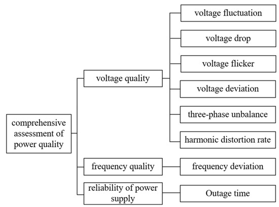
Figure 1.
Power quality evaluation system.
Various organizations have established standards for power quality. The International Electrotechnical Commission (IEC) standards and the European Standard [11] share significant similarities, while the Institute of Electrical and Electronics Engineers (IEEE) standards are primarily applied in North America. China has also developed its own national standards for power quality [12]. The definitions of the power quality assessment indicators adopted in this study are summarized in Table 1.

Table 1.
Table of definitions of power quality assessment indicators.
In Table 1, the subscript denotes the measured value, the subscript N represents the actual value, and is the weighting coefficient determined based on the human eye’s sensitivity curve to flicker (IEC 61000-4-15).
3. Combinatorial Empowerment Method
3.1. G1 Method
The G1 method, also referred to as ordinal relationship analysis, is a subjective weighting method developed from the Analytic Hierarchy Process (AHP). It assigns weights to indicators based on the ordinal relationships determined by decision-makers among different indicators. By doing so, it circumvents the consistency testing issue in the AHP and significantly reduces the computational burden while preserving the order.
Suppose there are n indicators, denoted as , , …, . The evaluator, based on personal experience, ranks the indicators in descending order of importance, obtaining the indicator attribute order relationship . For any two adjacent indicators, the degree of importance relationship can be expressed as follows:
In the formula, is the weight of , where = n, n − 1, …, 2. The larger the value of , the greater the importance of relative to . The values of and their corresponding meanings are presented in Table 2.
Table 2.
Scale and meaning of .
Based on the values of determined by the decision-maker, the subjective weight of each indicator is obtained by the following formula:
The subjective weights obtained according to the G1 method are = (, , …, ).
3.2. Improved CRITIC Method
The CRITIC method is an objective weighting approach. Its central concept is to reflect the amount of information contained in assessment indicators by introducing the contrast intensity and conflict degree. The contrast intensity is typically represented by the standard deviation. A larger standard deviation of the data implies greater fluctuations and a higher weight. The conflict degree is represented by the correlation coefficient. A larger correlation coefficient between indicators indicates a smaller conflict and a lower weight.
In this study, due to the non-uniform nature of the selected indexes, the standard deviation cannot be used to characterize the contrast strength. Therefore, the method requires improvement. This paper employs the coefficient of variation to characterize the comparative strength between indicators. A larger coefficient of variation indicates greater fluctuations and a higher weight. The method is as follows:
- Construction of the raw assessment indicator matrix X.
In the formula, represents the data of the nth indicator at the mth monitoring point.
- 2.
- Indicator normalization.
For positive indicators:
For reverse indicators:
In the formula, i = 1, 2, …, m; j = 1, 2, …, n.
- 3.
- Calculation of the coefficient of variation.
The mean value for each indicator is calculated:
The standard deviation for each indicator is calculated:
The coefficient of variation for each indicator is calculated:
In the formula, , , and represent the mean value, standard deviation, and coefficient of variation of the jth indicator.
- 4.
- Calculation of correlation matrix and conflict indicators.
The conflict degree is characterized by the correlation coefficient between indicators. The specific steps are as follows:
The correlation matrix R is calculated, where represents the correlation coefficient between the ith and jth indicators:
The conflict degree for each indicator is calculated:
In the formula, R is the correlation matrix, and represents the correlation coefficient between the ith and jth indicators.
- 5.
- Calculation of information content and weight values.
The information content is the product of the coefficient of variation and the conflict degree, reflecting the amount of information contained in each indicator. The weights are obtained by normalizing the information content:
The information content is calculated:
The objective weight is calculated:
The objective weights obtained through the improved CRITIC method are = (, …, ).
3.3. Combinatorial Empowerment Method Based on Game Theory
The combinatorial weighting method effectively integrates the subjective intentions of decision-makers with the objective relationships within the data, reflecting both the preferences of decision-makers for different indicators and the inherent patterns of the data. This results in more scientific and rational weighting outcomes. In this paper, we adopt the game theory-based combined weighting method, whose core idea is to treat subjective and objective weighting methods as two “players” within a game-theoretic framework. By optimizing strategies, we achieve synergy and equilibrium between the two, ultimately finding the optimal combination of subjective and objective weights—the Nash equilibrium point [13]. The specific implementation steps and integration mechanism of this method are as follows:
- Weight combination.
Let the weight vectors of the subjective weighting method (G1 method) and the objective weighting method (improved CRITIC method) be and , respectively, with their corresponding weight coefficients being and . The combined weight can be expressed as a linear combination of the two:
In the formula, and represent the contribution levels of the subjective and objective weights in the combination, respectively.
- 2.
- Nash equilibrium in the game theory framework.
To find the optimal combination of subjective and objective weights, we introduce the concept of game theory, treating the subjective and objective weights as two “players” whose goal is to minimize the difference between the combined weight and their respective weights. Specifically, the optimization problem can be formulated as follows:
In the formula, represents the weight vector of the pth player (i.e., subjective or objective weight), and denotes the Euclidean norm. The goal of this optimization problem is to make the combined weight as close as possible to both the subjective and objective weights, thereby achieving a balance between the two.
- 3.
- Solving the optimization problem.
Based on the properties of matrix differentiation, the optimization problem is transformed into a first-order derivative condition, yielding the following system of linear equations:
By solving this system of equations, the weight coefficients and can be obtained.
- 4.
- Normalization.
The optimal combination coefficients and are calculated and normalized:
The normalized coefficients and represent the relative importance of the subjective and objective weights in the final combination.
- 5.
- Calculation of the comprehensive weight.
Finally, the comprehensive weight is calculated as a linear combination of the normalized coefficients and the subjective and objective weights:
Under the framework of game theory, the integration of subjective and objective weights transcends mere linear superposition. Instead, it dynamically adjusts the contributions of both through equilibrium strategies. The resultant weights not only preserve the expertise embedded in the subjective method (G1 method) but also fully leverage the objective information derived from the data (enhanced CRITIC method). This approach effectively addresses the issue of imbalanced weight distribution inherent in traditional combined weighting methods, thereby achieving a more robust and scientifically grounded weighting scheme.
4. Improved Grey–TOPSIS Assessment Model
The TOPSIS method is a multi-objective decision-making evaluation approach. It ranks the advantages and disadvantages of all schemes by comparing the Euclidean distances between each evaluation scheme and the virtual optimal and worst solutions. However, the use of geometric distance alone can only reflect the positional relationship. When the degree of proximity is the same, it is impossible to determine the superiority or inferiority of the schemes. The grey correlation analysis method can better reflect the degree of correlation between variables. By combining it with the Euclidean geometric distance in the TOPSIS method, the relative positional relationship between assessments objects can be effectively identified, which makes up for the defects of the TOPSIS method. Therefore, this paper introduces the grey correlation analysis into the TOPSIS method. The specific steps are as follows:
- Standardize the original assessment index matrix X to obtain the standardized matrix .
- Calculate the weighted standardized matrix Y.
- 3.
- Determine the positive ideal and negative ideal , which are, respectively, the sets of maximum and minimum values corresponding to each indicator in the weighted normalized matrix Y.
- 4.
- Calculate the Euclidean distance and grey correlation degree.
Calculate the Euclidean distances and from each evaluation object to the positive ideal solution and negative ideal solution:
Calculate the grey correlation coefficients and :
In the formula, is the discrimination coefficient. It typically assumes values within the interval (0,1], and a commonly used value for it is ρ = 0.5.
In response to composite system behavior, a sensitivity discrimination coefficient for localized data fluctuations is proposed.
In the formula, is the global standard deviation.
Calculate the grey correlation degrees and between the ith solution and the positive and negative ideal solutions, respectively.
- 5.
- Fit the grey correlation to the Euclidean distance criterion and define the new characteristic quantity and . These two quantities represent the degree of proximity to the ideal solution and the degree of deviation from the ideal solution, respectively. A larger value of indicates a better performing solution, while a larger value of implies a worse performing one.
In the formula, represents the evaluator’s preference degree for the location pattern. When there is no subjective preference, τ is usually set to 0.5.
- 6.
- Calculate the relative closeness of the program. A larger value indicates that the program is better, and conversely, a smaller value means the program is worse.
5. Example Analysis
This case study analyzes data from 36 monitoring points within a wind farm grid-connection area, obtained from a municipal power quality monitoring system. The dataset spans from January to December 2024 with a sampling frequency of 15 min intervals. All acquired data underwent denoising and normalization preprocessing, with the processed results provided in Appendix A. The selected indicators are the voltage deviation rate, harmonic distortion rate, voltage flicker rate, frequency deviation, three-phase unbalance degree, and voltage fluctuation, respectively.
- G1 method.
Five wind power experts were invited to rank the importance of six indicators based on their expertise, establishing a consensus ordinal relationship: . The relative weights among evaluation indicators were then determined according to the scale definitions in Table 1: = 1.6, = 1.4, = 1.8, = 1.2, and = 1.2.
Based on Equations (2) and (3), the subjective weights of the power quality indicators were as follows:
- 2.
- Improved CRITIC method.
According to Equations (7)–(9) and (11), the standard deviation , mean value , coefficient of variation , and conflict index of each power quality indicator were calculated as follows:
Based on Equation (13), the objective weights of each power quality indicator were as follows:
- 3.
- Combinatorial empowerment method based on game theory.
The subjective weights and objective weights were integrated through Equations (14)–(17), yielding the optimized coefficients = 0.9061 and = 0.0939. The comprehensive weights for the power quality indicators were subsequently derived as follows:
- 4.
- Improved grey–TOPSIS assessment model.
The model was employed to solve the problem. The relative closeness of each monitoring point to the power quality in terms of the integrated rank order of superiority and inferiority was calculated, and the results are shown in Table 3.
Table 3.
Relative closeness of monitoring points and ranking of power quality by merits and demerits.
To validate the effectiveness of the proposed method, a comparative analysis was conducted against existing approaches from the literature. To ensure fairness in comparison, all parameters of the benchmark methods were re-optimized based on the dataset used in this study. In the CRITIC-TOPSIS model from Reference [14], the correlation coefficient of the evaluation index matrix was adjusted to 0.7 (originally 0.6) via grid search optimization to better align with the high-volatility characteristics of wind power data. For the Lagrange–VIKOR model in Reference [15], the Lagrange multiplier λ was optimized to 0.62 (originally 0.5) through gradient descent minimization of weight deviation. In the weighted rank-sum ratio method of Reference [16], the linear weighting function was modified to a logarithmic form to enhance compatibility with non-uniform data distributions. The comprehensive rankings of power quality performance across monitoring points, derived from these parameter-optimized methods, are illustrated in Figure 2.
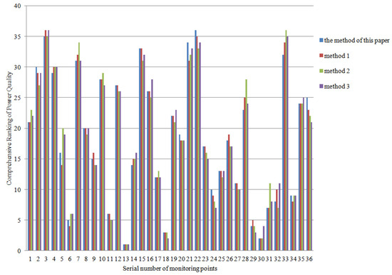
Figure 2.
Rankings of comprehensive power quality merits and demerits of monitoring points under different schemes.
As is evident from Figure 2, the results obtained by the method proposed in this paper are generally consistent with those of the assessment methods employed in References [14,16]. Only minor discrepancies emerge in the evaluation of certain individual monitoring points. Method 1 [14] employs a CRITIC-TOPSIS integrated evaluation approach that relies on raw data information, emphasizing inter-data correlations and conflicts. In contrast, our method undermines objectivity by incorporating the G1 method to refine data weighting, thereby achieving more scientifically robust evaluation results. With under 5% Gaussian noise injection, the method proposed in this paper demonstrates a Kendall’s coefficient of 0.85, outperforming the 0.74 reported in Reference [14], which confirms superior ranking consistency. Method 2 15 adopts the Lagrange multiplier method to combine subjective and objective weights, deriving a compromised solution through maximizing collective benefits and minimizing individual losses. However, this approach exhibits strong subjectivity and high computational complexity. In this paper, we employ the game theory method to assign subjective and objective weights. Within the Matlab computing environment, the computation time is 4.7 s, significantly lower than the 12.7 s reported in Reference [15]. This reduces computational complexity while balancing the subjectivity and objectivity of weight allocation, yielding more reasonable evaluation results. Method 3 [16] uses the weighted rank-sum ratio method to evaluate power quality. Although the calculation based on ranking can, to some extent, mitigate the interference of outliers, it may still impact the overall distribution characteristics of the data. The grey–TOPSIS method adopted in this paper fully exploits the original data, preserves the original data information, and reflects the power quality advantages and disadvantages of the monitoring points through the magnitude of the relative closeness, ensuring high data accuracy.
The abovementioned study enables the ranking of the power quality of multiple monitoring nodes within the monitoring system. Nevertheless, when it comes to assessing the power quality of the monitoring nodes, national standard data should be incorporated into the model. The Chinese standard classifies power quality into five distinct levels [17], namely excellent, good, medium, qualified, and unqualified. The classification ranges and the corresponding relative closeness value ranges obtained through the model solution are presented in Table 4.
Table 4.
Power quality grade classification and the ranges of corresponding relative closeness values.
For monitoring points with unqualified power quality, the power sector should conduct strict monitoring. Based on the specific conditions of the indicators at these points, relevant management measures should be taken in a timely manner to address power quality issues. For qualified and medium-level monitoring points, the power sector needs to pay close attention and conduct regular monitoring to prevent the further deterioration of power quality, which could otherwise lead to significant losses. For good- and excellent-level monitoring points, the power sector can carry out regular inspections according to the actual electricity demand, thereby saving technical and economic costs.
The aforementioned evaluation results validate the effectiveness of the proposed method under single-disturbance scenarios. However, in practical power grids, wind power integration-induced power quality issues frequently exhibit coupled multi-disturbance characteristics, such as harmonic distortion superimposed with voltage flicker and coexisting frequency deviations with voltage fluctuations. Such compound disturbances not only exacerbate equipment degradation but may also cause misjudgments in conventional assessment methods due to rigid weight allocation. To address this, we further designed multi-disturbance experimental scenarios to verify the model’s robustness under complex operating conditions and conducted comparative analyses against existing methodologies.
In this study, a representative compound disturbance scenario combining harmonic distortion and voltage flicker was generated using field-measured data. Specifically, we considered the following:
Harmonic injection: third-order (150 Hz) and fifth-order (250 Hz) harmonics were introduced with amplitudes of 3% and 2% of the fundamental component, respectively, achieving a total harmonic distortion (THD) of 3.6%.
Voltage flicker generation: a rectangular modulation waveform with 10% depth and 8.8 Hz frequency was applied, resulting in a short-term flicker severity () of 1.05.
Based on evaluation data from 36 monitoring points, Figure 3 illustrates the relative closeness index () of different methods for the high-performance monitoring point 13, while Table 5 compares their performance metrics under this compound disturbance scenario.
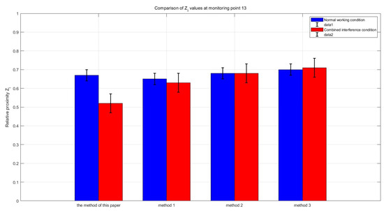
Figure 3.
Relative proximity change of monitoring point 13.
Table 5.
Performance indexes of different methods in the composite disturbance scenario.
As can be seen from Figure 3, after injecting compound disturbances at monitoring point 13, the relative closeness index of the proposed method decreased from 0.67 to 0.52, corresponding to a “moderate” power quality classification in Table 5. In contrast, the other methods maintained higher values due to their lack of dynamic weight adjustment, resulting in the misclassification of power quality levels. Table 5 shows that the proposed method demonstrates significant advantages in both ranking accuracy and noise immunity, maintaining high precision under compound disturbances, which confirms its robustness and practicality in power quality assessment for wind power integration.
6. Conclusions
Based on the grid integration characteristics of wind power, this paper establishes a power quality evaluation system suitable for wind power integration systems. By considering key criteria, the voltage deviation rate, harmonic distortion rate, voltage flicker rate, frequency deviation, three-phase unbalance degree, and voltage fluctuation rate, the system comprehensively assesses power quality issues in wind power integration systems. The G1 method and an improved CRITIC method are combined through game theory for weighting, effectively integrating the information inherent in the data with subjective expert evaluations. This approach resolves the imbalance between subjective and objective weights in wind power scenarios. The grey–TOPSIS method is applied to evaluate power quality, utilizing the concept of relative closeness to rank or qualitatively classify power quality levels. Comparative analyses with existing methods and evaluations under composite disturbance scenarios collectively validate the rationality and accuracy of the proposed methodology.
Additionally, the method demonstrates a degree of adaptability. Given the geographical and regulatory differences in wind power integration systems, if a region experiences strong wind power volatility, the weight of voltage fluctuation can be flexibly adjusted using the G1 method to align the evaluation results with the geographical environment. Similarly, if a region’s grid imposes strict limits on harmonics, the harmonic distortion rate indicator can be expanded to include both harmonic and inter-harmonic distortion rates, ensuring that the evaluation results comply with regional grid requirements, thus offering practical value.
Although this study demonstrates several strengths, it is important to acknowledge certain limitations. Firstly, the methodology depends significantly on the selected evaluation criteria, in this case, primarily focusing on voltage quality and frequency quality metrics. However, in actual grid operation, power supply reliability indicators constitute an equally critical technical parameter that cannot be overlooked. Additionally, although the grey–TOPSIS method mitigates uncertainty to some extent, the dependence on expert judgment during the weighting process may introduce subjectivity. This subjectivity could influence the final evaluation outcomes, as different experts might prioritize criteria based on personal or regional perspectives. Lastly, while the grey–TOPSIS method accommodates imprecision, it may not fully address the dynamic fluctuations in power quality induced by climate change in wind power integration systems, which could affect the long-term sustainability of the proposed approach.
Based on these limitations, future research directions are suggested. The selection of evaluation indicators should extend beyond technical metrics to include economic and stability indicators, which are also of significant practical relevance in real-world grid operations. For addressing the strong time-varying nature of power quality, the introduction of a real-time weight adjustment mechanism is recommended. By employing a sliding window mechanism to dynamically adjust weights, the model’s adaptability to fluctuations in wind power output can be enhanced, facilitating more effective real-time decision-making.
Author Contributions
Conceptualization, T.Q. and L.Y.; methodology, T.Q. and L.Y.; software, L.Y.; validation, T.Q. and L.Y.; formal analysis, T.Q.; investigation, T.Q.; resources, L.Y.; data curation, T.Q. and L.Y.; writing—original draft preparation, T.Q.; writing—review and editing, L.Y.; visualization, T.Q.; supervision, L.Y.; project administration, L.Y.; funding acquisition, T.Q. and L.Y. All authors have read and agreed to the published version of the manuscript.
Funding
This research received no external funding.
Data Availability Statement
The original contributions presented in the study are included in the article.
Conflicts of Interest
The authors declare no conflict of interest.
Appendix A. Power Quality Index Data of 36 Monitoring Points
| Node | /% | /% | /Hz | /% | /% | |
| 1 | 4.764506 | 2.366283 | 0.683749 | 0.887486 | 1.925419 | 1.091824 |
| 2 | 5.440806 | 0.861006 | 0.736075 | 0.140365 | 1.830416 | 1.045692 |
| 3 | 1.692084 | 3.382496 | 0.57002 | 0.595364 | 0.873536 | 1.79686 |
| 4 | 6.95887 | 0.589387 | 0.926546 | 0.5577 | 0.366262 | 1.858256 |
| 5 | 6.589324 | 1.561121 | 0.018817 | 0.070832 | 0.629426 | 0.147472 |
| 6 | 6.684685 | 1.016866 | 0.672682 | 0.076607 | 0.992273 | 0.372064 |
| 7 | 6.023566 | 0.278984 | 0.123736 | 0.904869 | 1.714442 | 0.487539 |
| 8 | 2.124306 | 2.859197 | 0.724434 | 0.786743 | 0.453666 | 0.290274 |
| 9 | 2.453549 | 2.923617 | 0.524734 | 0.971014 | 0.717085 | 1.935821 |
| 10 | 1.525897 | 2.872063 | 0.837761 | 0.069741 | 1.984114 | 1.516539 |
| 11 | 3.040983 | 2.704715 | 0.075846 | 0.519548 | 1.536642 | 1.74504 |
| 12 | 6.488077 | 2.824535 | 0.456925 | 0.539166 | 0.311698 | 0.26496 |
| 13 | 6.89117 | 1.839148 | 0.107309 | 0.105406 | 1.516044 | 0.785506 |
| 14 | 1.64983 | 1.869453 | 0.110314 | 0.069352 | 1.08383 | 1.466838 |
| 15 | 4.368363 | 0.188689 | 0.796814 | 0.2908 | 0.523938 | 0.655554 |
| 16 | 1.744469 | 3.835728 | 0.688078 | 0.929123 | 0.762905 | 1.993858 |
| 17 | 5.585262 | 2.179783 | 0.147189 | 0.457918 | 0.43461 | 1.625358 |
| 18 | 1.287231 | 0.080998 | 0.77072 | 0.906383 | 0.798355 | 0.021789 |
| 19 | 5.358476 | 0.753136 | 0.142697 | 0.304356 | 0.367686 | 1.719695 |
| 20 | 1.93266 | 1.805338 | 0.962497 | 0.842241 | 1.236403 | 0.762215 |
| 21 | 3.75914 | 0.518277 | 0.203793 | 0.419845 | 0.665465 | 1.003892 |
| 22 | 5.544837 | 2.7914 | 0.725044 | 0.77581 | 1.006825 | 1.291138 |
| 23 | 4.971233 | 2.757394 | 0.028075 | 0.425342 | 1.796824 | 0.900637 |
| 24 | 1.322146 | 3.922444 | 0.739152 | 0.753825 | 0.605623 | 1.821617 |
| 25 | 4.591464 | 2.125706 | 0.470407 | 0.758699 | 0.988231 | 1.165839 |
| 26 | 3.343216 | 1.097493 | 0.787555 | 0.254113 | 1.690028 | 1.366347 |
| 27 | 4.477466 | 0.012044 | 0.469906 | 0.286539 | 0.112711 | 0.576306 |
| 28 | 5.469958 | 1.309823 | 0.977772 | 0.75288 | 1.59006 | 1.605036 |
| 29 | 4.79009 | 3.920886 | 0.187101 | 0.93789 | 1.553346 | 0.499191 |
| 30 | 4.466729 | 2.861963 | 0.345485 | 0.441199 | 1.233763 | 0.053518 |
| 31 | 2.931752 | 2.464464 | 0.574255 | 0.654148 | 0.942301 | 1.606782 |
| 32 | 3.369503 | 1.928264 | 0.007127 | 0.212553 | 1.506684 | 1.729219 |
| 33 | 4.575386 | 1.945666 | 0.974714 | 0.235809 | 1.631835 | 0.757311 |
| 34 | 3.589589 | 2.303674 | 0.608 | 0.326103 | 1.723664 | 1.603347 |
| 35 | 5.019921 | 0.335389 | 0.685207 | 0.807456 | 0.748011 | 0.79564 |
| 36 | 4.131763 | 3.832771 | 0.943784 | 0.022013 | 0.512597 | 1.798764 |
References
- Bai, H.; Wang, R. Analysis of the Influence of Wind Farm Grid-connection on Power Grid Power Quality. Proc. CSU–EPSA 2012, 24, 120–124. [Google Scholar]
- Wang, Y.; Du, W.; Wang, H. Sub-synchronous Oscillation Frequency Drift Problem in Wind Power Grid-connected Systems. Trans. China Electrotech. Soc. 2020, 35, 146–157. [Google Scholar]
- Xiao, B.; Zhao, X.; Dong, G. Review and Prospect of Comprehensive Assessment Methods for Power Quality. J. Power Gener. Technol. 2024, 45, 716–733. [Google Scholar]
- Zeng, Q.; Yang, H.; Yang, X.; Zhou, N.; Li, H. Comprehensive Assessment of Power Quality Considering Index Correlation. Proc. CSU–EPSA 2016, 28, 73–78. [Google Scholar]
- Lu, Y. Comprehensive Assessment of Power Quality Based on Improved Extension Analytic Hierarchy Process. Softwave 2019, 40, 16–20. [Google Scholar]
- Zhang, T.; Cheng, Z.; Liang, D.; Wang, N.; Xia, J. Application of Nonlinear Principal Component Analysis in Comprehensive Assessment of Power Quality. Electr. Meas. Instrum. 2008, 45, 5–9. [Google Scholar]
- Zhang, M.; Xia, R.; Xu, S.; Lu, D.; Hu, Y. Comprehensive evaluation method of power quality based on combined weighting of subjective and objective variation coefficients. Mod. Electr. Power 2023, 40, 441–447. [Google Scholar]
- Li, J. Research on Power Quality Evaluation Method Based on Cooperative Game and Improved TOPSIS. Power Syst. Prot. Control 2018, 46, 109–115. [Google Scholar]
- Tang, M.; Li, R.; Cheng, X.; Dai, X.; Yu, X. Adaptability Assessment of New Energy Power System Based on Game Theory-Improved Cloud Model. Power Syst. Prot. Control 2025, 53, 40–51. [Google Scholar] [CrossRef]
- Zhao, Y.; Zhou, H.; Wang, Y.; Li, H.; Sun, M. Research on Power Quality of Wind Power Grid-connected System Based on Fuzzy Comprehensive Evaluation. Renew. Energy Resour. 2023, 41, 1368–1375. [Google Scholar]
- BS EN 50160:2007; Voltage characteristics of electricity supplied by public distribution networks. British Standards Institution: London, UK, 2007.
- GB/T 15945-2008; Power Quality—Deviation of Power Frequency. Standardization Administration of China: Beijing, China, 2008.
- Marden, J.; Shamma, J. Game Theory and Control. Annu. Rev. Control Robot. Auton. Syst. 2018, 1, 105–134. [Google Scholar] [CrossRef]
- Lv, Z.; Wu, M.; Song, Z.; Zhao, T.; Du, G. Comprehensive evaluation of power quality on CRITIC-TOPSIS method. J. Electr. Mach. Control 2020, 24, 137–144. [Google Scholar]
- Qian, J.; Li, H.; Li, G.; Zhang, Y.; Wang, Q. Comprehensive Power Quality Assessment Based on Combined Weighting-VIKOR. Electr. Drive 2024, 54, 37–44. [Google Scholar]
- Fu, X.; Chen, H. Comprehensive Evaluation of Power Quality Based on the Weighted Rank-Sum Ratio Method. J. Power Autom. Equip. 2015, 35, 128–132. [Google Scholar]
- Zhou, L.; Li, Q.; Zhang, F. Application of Genetic Projection Pursuit Interpolation Model in Comprehensive Power Quality Assessment. Power Syst. Technol. 2007, 31, 32–35. [Google Scholar]
Disclaimer/Publisher’s Note: The statements, opinions and data contained in all publications are solely those of the individual author(s) and contributor(s) and not of MDPI and/or the editor(s). MDPI and/or the editor(s) disclaim responsibility for any injury to people or property resulting from any ideas, methods, instructions or products referred to in the content. |
© 2025 by the authors. Licensee MDPI, Basel, Switzerland. This article is an open access article distributed under the terms and conditions of the Creative Commons Attribution (CC BY) license (https://creativecommons.org/licenses/by/4.0/).