
Formal Verification of Autonomous Vehicle Group Control Systems via Specification Translation of Multitask Hybrid Observational Transition Systems


Abstract
1. Introduction
2. The Multitask Hybrid Observational Transition Systems
2.1. Definition of MHOTS
- : A set of observers.The set = is classified into a set of global discrete observers; , local discrete observers; , global continuous observers and , local continuous observers.Each global observer is a function , where is a data type. Similarly, each local observer is a function . We write instead of , and we denote as an element of and for and if no confusion occurs. The equivalence relation between two states is defined as the observational equivalence, i.e., if and only if . . has a special master clock that observes the elapsed time since the execution of began.
- : A set of initial states such that .
- : A set of transitions.is divided into a set of global discrete transitions, a set of local discrete transitions, and a set of continuous transitions. Each (or ) is a function (or ). For and , we may write and , respectively, if no confusion occurs. All transitions preserve , that is, whenever . Every transition τ has an effective condition defined as . For , its effective condition is given as a function (or ). If (or ) is false then (or ). has only one special continuous transition , that is, , called a time advancing transition. If and it is effective, then = for each and .
- For each continuous observer , we define a flow constraint for global ones, or for local ones, which constrains the evolution of the values of o, that is, (or ) returns the value observed by o (or ) after time t from state s.
- For discrete observers , we call a tuple of all their observed values a location. The set of locations is defined as
- For each observer (or ), we assume there is a corresponding symbol (or ), which is called a variable in ordinary hybrid automata. We denote the set of all such variables by X.
- We define an invariant for each location, where the hybrid system can stay at the location as long as the invariant is true. An invariant function gives the evolution domain restriction , called an invariant condition of location , where is the class of polynomial constraints over the set of continuous variables X. For example, is a polynomial constraint over . For and a valuation v : where D is the union of all , a boolean value is the result of replacing x with . For example, for a valuation υ such that , the boolean value is false.We assume is a conjunction of for all and , that is, = , where .
- The time advancing transition should satisfy the following conditions: for , for and for whenever is true.
- The effective condition is defined as follows: if and only if. . ∧ ∧ ⇒ , and. . ∧ ∧ ⇒Roughly speaking, is effective when all of the invariant conditions hold with the values of the continuous observers after time t, that is, .
2.2. Illustrative Example of MHOTS: A Two-Tank Water Flow System
- : ObserversDiscrete Observers (): valve state ∈ indicating the status of the valve connecting two tanks.Continuous Observers (): level A ∈ ≥ 0: Water level in Tank A; level B ∈ ≥ 0: Water level in Tank B; now ∈ ≥ 0: Global system time.
- : The initial conditions of the state.The initial valve state is closed: valve(init) = closedTank A and Tank B initial water levels: levelA(init) = 10, levelB(init) = 2.Initial system time: now(init) = 0.
- : TransitionsContinuous transitions are governed by the following set of differential equations: When the valve is open:When the valve is closed:Here, the constant k represents the water flow velocity (assumed to be unit/s). So the next function can be defined followingWhen the valve is open:When the valve is closed:Time Observer:The position invariant constraint is that the water levels of Tank A and Tank B must always satisfy:Therefore, the effective condition for continuous migration is as follows:Define the following valve state transition rules (discrete transitions):Open valve:Transition condition: Tank B water level is lower than the lower threshold (e.g., levelB ≤ 3).Behavior: The valve changes from closed to open.Close valve:Transition condition: The water level of Tank B reaches the upper threshold (for example, levelB ≥ 8).Behavior: The valve changes from open to closed.At this time, the water level (levelA, levelB) and time (now) do not change.
2.3. Fundamental Assumptions of MHOTS
- Velocity update: .
- Position update: .
3. Multitask Hybrid OTS/CafeOBJ Specifications
3.1. Specification of Sets of Processes
mod* PID{
  [Pid]
  pred _=_ : Pid Pid {comm}
  var P : Pid
  eq (P = P) = true .
}
mod! PSET{
  pr(PID)
  [Pid < PSet]
  op nil : -> PSet
  op _ _ : PSet PSet -> PSet {assoc idr: nil}
  op dummy : -> Pid
  pred _in_ : Pid PSet
  pred empty : PSet
  op first : PSet -> Pid
  op last : PSet -> Pid
  op _sub_ : PSet PSet -> Bool
  op ps : -> PSet
  …
}
3.2. System Description of MHOTSs in CafeOBJ
- :: =
- :: = mod(!|*)
- :: = mod* M {
- pr(S )… pr(S )
- *[H]*
- ::= …
- ::= op init : .
- ::= … …
- ::= eq (init) = .
- ::= eq (init,) = .
- ::= bop : H
- ::= bop : H
- ::=
- ::= bop : H
- ::= bop : H → Bool
- ::= bceq (S,) = S if not (c-(S,)).
- ::= ceq ((S,)) = ’ if c-(S,).
- ::= ceq ((S,), ) = ’ if c-(S,).
- ::= … …
- ::= vars S: H
- ::= vars :
- ::= vars:
- }
3.3. A Case Study of the MHOTS/CafeOBJ Method
ops start accel nothing brake : -> Label
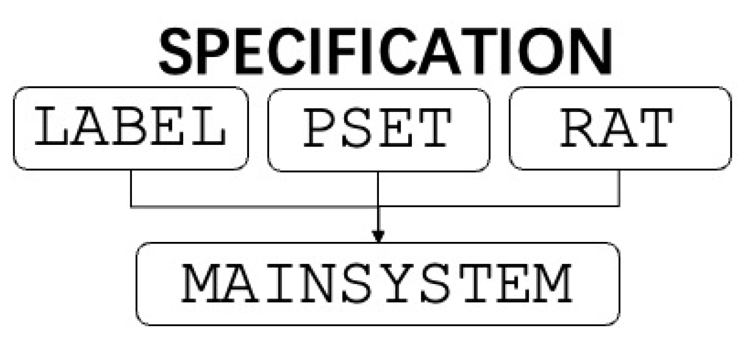
mod* MAINSYSTEM{
  pr(PSET + RAT + LABEL)
 …
 eq v(P,init) = 0 .   eq x(P,init) = 0 .   eq now(init) = 0 .
 eq loc(P,init) = start .  eq ps(init) = nil .
eq c-enter(P,S)= (loc(P,S) = start) and (ps(S) = nil or x(last(ps(S)),S) > 0) .
ceq ps(enter(P,S))= P ps(S) if c-enter(P,S) .
ceq loc(P',enter(P,S))= (if P' = P then accel else loc(P',S) fi) if c-enter(P,S) .
eq v(P',enter(P,S))= v(P',S) . eq x(P',enter(P,S))= x(P',S) .  …
where the first equation specifies that enter is effective when the location is start and either the set of entered vehicles is empty or the last vehicle of the set is not at position 0. Only ps and loc are changed by enter, while the other observed values remain unchanged. The value of ps at the state after applying enter, that is, ps(enter(P,S)), is the set P ps(S) obtained by adding P at the end of the original set ps(S). Only the P’s location is updated to accel by enter(P,S). We omitted the transitions a b and n similar to enter.
eq loc(P,tick(T,S)) = loc(P,S) .
ceq v(P,tick(T,S)) = (if loc(P,S) = start then 0 else nextv(P,T,S) fi)
                     if c-tick(T,S) .
ceq x(P,tick(T,S)) = (if loc(P,S) = start then 0 else nextx(P,T,S) fi)
                     if c-tick(T,S) .
eq nextv(P,T,S) = v(P,S) + ac(loc(P,S)) * T .
eq nextx(P,T,S) = v(P,S) * T + 1/2 * ac(loc(P,S)) * T * T + x(P,S) .
eq ps(tick(T,S)) = ps(S) .
where the acceleration value of the vehicle is defined for each location by operation ac, where accel, brake, and nothing are 1, , and 0, respectively. The values of v and x after tick are defined as the next values of them when the locations are not start. Note that we specify that the values of v and x are always 0 at the location start. As the system time advances (tick(T, S)), the state of ps (which is a queue of all vehicles) remains unchanged.
eq c-tick(nil,T,S) = true.
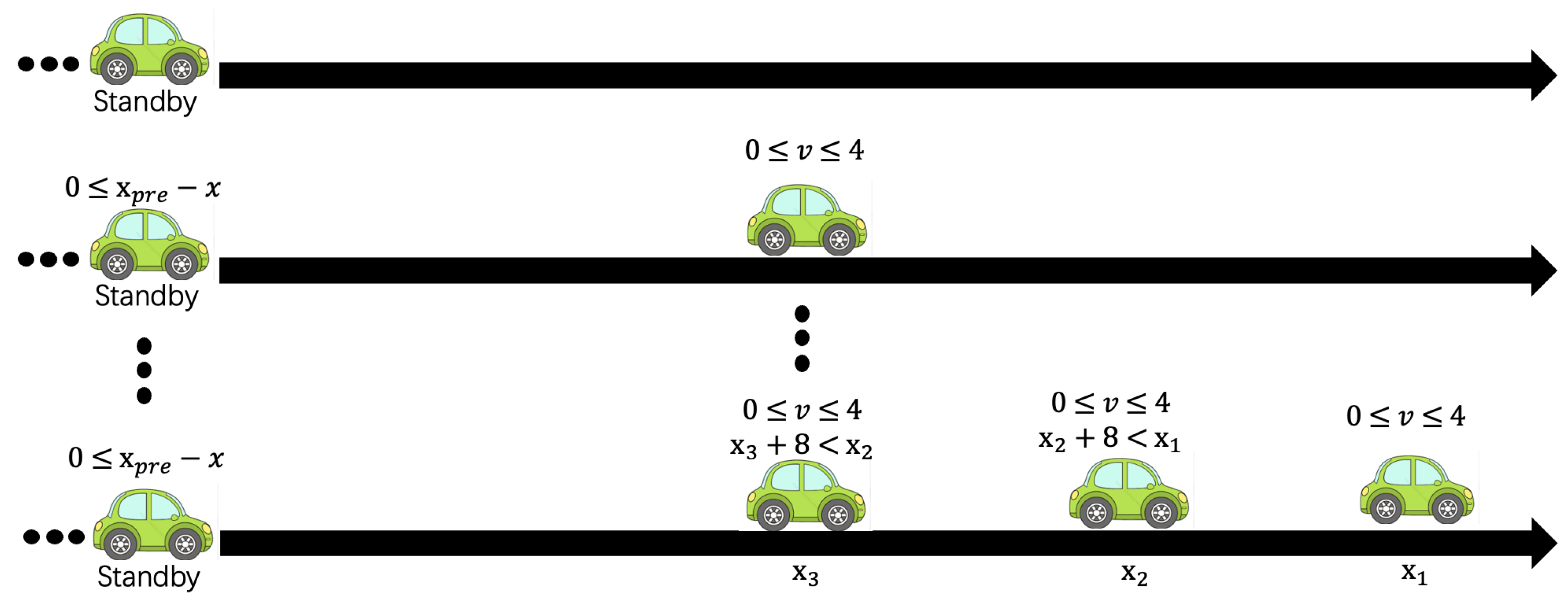
eq c-tick(P,T,S) = ((loc(P,S) = brake or loc(P,S) = accel or loc(P,S) = nothing)
implies (0 <= nextv(P,T,S) and nextv(P,T,S) <= 4)) .
eq c-tick(P Q,T,S) = c-tick(Q,T,S) and c-tick(P,T,S) and
(loc(P,S) = accel implies (nextx(P,T,S) + 8 < nextx(Q,T,S)))
and (loc(P,S) = nothing implies (((0 < nextv(P,T,S) and
nextv(P,T,S) <= 4) and (nextx(P,T,S) + 8 < nextx(Q,T,S))))
or nextv(P,T,S) = 0) .
eq c-tick(P Q PS,T,S) = c-tick(P Q,T,S) and c-tick(Q PS,T,S) .
eq c-tick(T,S) = c-tick(ps(S),T,S) .
4. Verification of the Theorem Proving
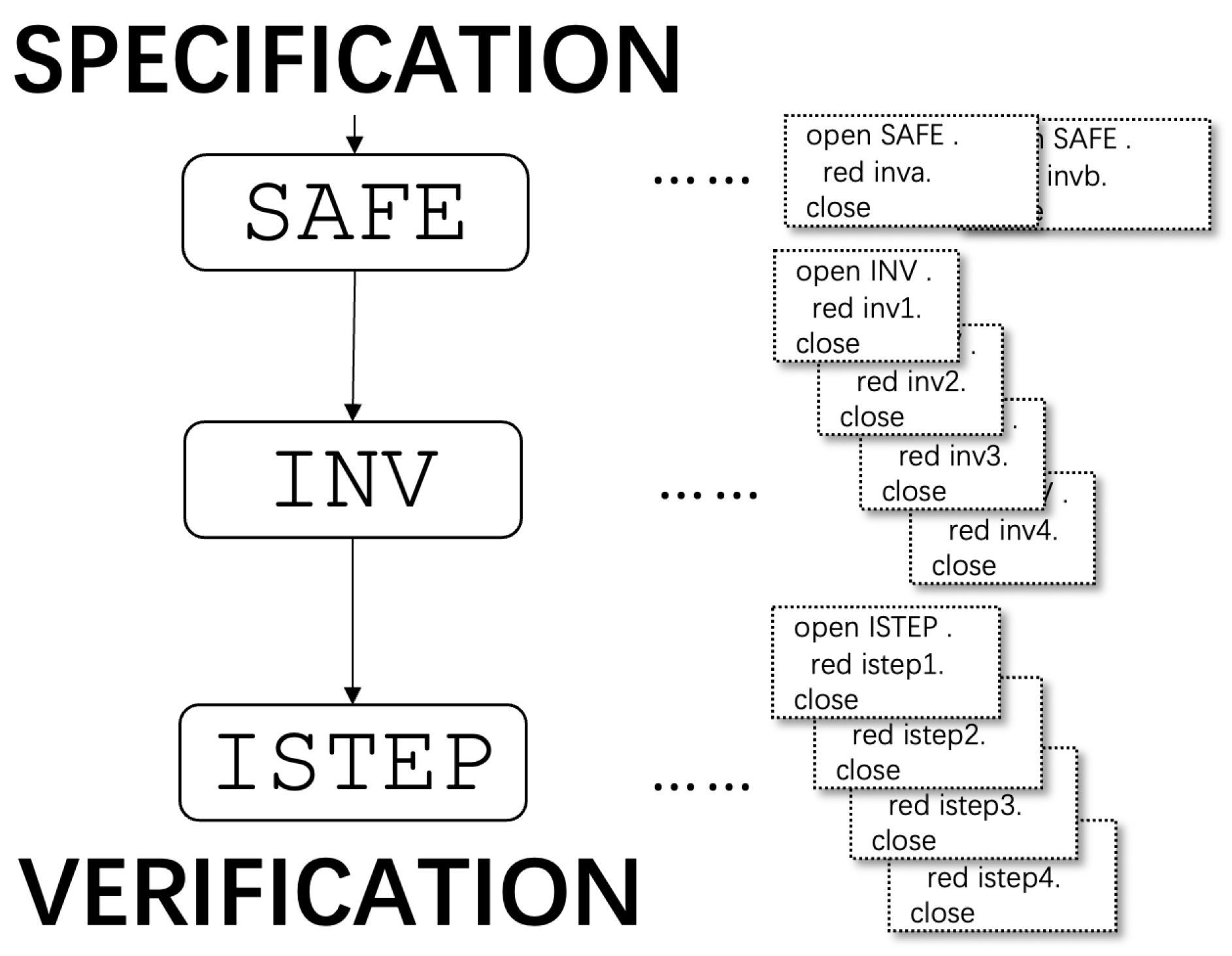
4.1. Module for the Safety Property
  eq safe(nil,S) = true .
  eq safe(P,S) = true .
  eq safe(P Q,S) = (x(P,S) < x(Q,S)) .
  eq safe(P Q PS,S) =
  safe(P Q,S) and safe(Q PS,S) .
4.2. Induction Basis
eq inv1(Q,Q',QS',S) = (Q Q' QS' sub ps(S) implies (x(Q,S) < x(Q',S))) .
open INV .
    red inv1(q,q',qs',init) .
close
4.3. Induction Step
eq istep1 = inv1(s) implies inv1(s') .
open ISTEP .
    op t1 : -> Rat .
    eq s' = tick(t1,s) .
    red istep1 .
close
open ISTEP .
    op t1 : -> Rat .
    eq c-tick(t1,s) = false .
    eq s' = tick(t1,s) .
    red istep1 .
close
open ISTEP .
    op t1 : -> Rat .
    eq c-tick(t1,s) = true .
    eq s' = tick(t1,s) .
    red istep1 .
close
4.4. Lemma Introduction
eq inv2(P,S) = (loc(P,S) = start implies x(P,S) = 0) .
eq istep2 = inv2(s) implies inv2(s') .
red inv2(s) implies istep1 .
eq inv1(Q,Q',QS',S) = (Q Q' QS' sub ps(S) implies (x(Q,S) < x(Q',S))) .
eq inv2(P,S) = (loc(P,S) = start implies x(P,S)=0) .
eq inv3(P,S) = (P in ps(S)) implies (not loc(P,S) = start) .
eq inv4(Q,Q',QS',S) = (Q Q' QS' sub ps(S) implies (x(Q,S) < (- 1/2 * v(Q,S)
* v(Q,S)) + x(Q',S))) .
5. Specification Translation to Real-Time Maude
5.1. Specification Translation
- =
- = (fmod … endfm)
- = (tmod M is
- pr . … pr .
- =
- = op : → System.
- = op : → OValue.
- = op c-: System → Bool.
- =
- = crl [ ]: … … ’ … ’ …if c-.
- = eq init = … …
- endtm)
- Step 1: Identification and Preparation of Modules.CafeOBJ: Identify the main system module and all submodules, including data modules (e.g., LABEL, PID, PSET).Real-Time Maude: Correspondingly define a Real-Time Maude functional module (fmod) for each CafeOBJ data module and a system module (tmod) for the CafeOBJ system module.
- Step 2: Sorts and Subsorts TranslationTranslate CafeOBJ sorts to Real-Time Maude sorts.Declaring subsort relationships explicitly in Real-Time Maude using the subsort keyword to maintain sort hierarchies.
- Step 3: Operator TranslationTranslate CafeOBJ operators (op) to Real-Time Maude operators, preserving the arity and type signature. For example, a CafeOBJ observer is defined as follows:translates into Real-Time Maude as follows:
- Step 4: Initial State TranslationTranslate the CafeOBJ initial state (e.g., eq init = …) into Real-Time Maude as an equation defining the initial configuration of the system. For example, from cafeobjTranslate into Real-Time Maude:
- Step 5: Transition TranslationTranslate CafeOBJ transitions (defined by equations and conditional equations) into Real-Time Maude rewrite rules (rl, crl).The effective condition of transitions (c-) in CafeOBJ is explicitly translated into the condition part of conditional rewrite rules (if c-) in Real-Time Maude. For example, from cafeobjTranslate into Real-Time Maude:
- Step 6: Consistency Check and VerificationPerform initial consistency checks by simulation using Real-Time Maude (trew command). Apply Real-Time Maude model checking (tsearch command) to verify safety properties and discover potential errors.
| Algorithm 1: TranslateSpec (CafeOBJ_Spec) |
| Input: CafeOBJ_Spec Output: Real-Time Maude_Spec 1. Extract all submodules from CafeOBJ_Spec. 2. For each submodule: a. Map sorts and operators to Real-Time Maude format. b. For each transition with effective condition c-: : Define corresponding rewrite rule in Real-Time Maude: crl [] : PreState => PostState if c- holds. 3. For each predicate used in verification: Map to equivalent Real-Time Maude boolean functions. 4. Assemble all mapped modules into the final Real-Time Maude_Spec. 5. Return Real-Time Maude_Spec. |
5.2. A Case Study of the MHOTS/Real-Time Maude Method
(fmod LABEL is
  sort Label .   ops start accel nothing brake : -> Label . ...
endfm)
ops indicates the definition of multiple operators, that is, symbolic constants that can be represented. start, accel, nothing, brake are the names of labels, representing the four control states of the vehicle.
(tmod MAINSYSTEM is including (LABEL + PSET) .
  protecting POSRAT-TIME-DOMAIN .
  protecting RAT .
  sort OValue .
  subsorts Label < OValue < System .
  op loc : Pid Label -> OValue .
  ops v x : Pid Rat -> OValue .
  op init : -> System .
  eq init(P) = (v(P,0)x(P,0))loc(P,start) .
  ...
 endtm)
loc(P, L) represents the location of process P, represented by label L. Pid represents the unique identifier of the process (Process Identifier). v(Pid, Rat) and x(Pid, Rat) represent the velocity and position coordinates of process P, respectively. init defines the initial state of the system. System represents the state type of the entire system. init(P) means that the initial velocity and initial position are 0, and the initial state label is the initial state of the system of start. The local observations defined in the OTS/CafeOBJ specification are translated into operations : → of Real-Time Maude. For example, loc(P, start) is a term of the sort OValue.
 crl [a] : loc(P,L) => loc(P,accel) if not (L = start) .
 crl [b] : loc(P,L) => loc(P,brake) if not (L = start) .
 crl [n] : loc(P,L) => loc(P,nothing) if not (L = start) .
 rl [enternil] : (loc(P,start)ps(nil)) => (loc(P,accel)ps(P)) .
 crl [enterPS] : ((loc(P,start)ps(Q PS))x(Q,X)) => ((loc(P,accel)ps(P Q PS))
 x(Q,X)) if (0 < X) .
 eq update(T,((loc(P,L)v(P,V))x(P,X))OVS) =
 ((loc(P,L)v(P,nextv(L,P,T,V)))x(P,nextx(L,P,T,V,X)))update(T,OVS) .
 crl [tick] : {OVS} => {update(T,OVS)} in time T if c-tick(T,OVS) .
 eq c-tick(nil,T,OVS) = true .
 eq c-tick(T,ps(PS)OVS) = c-tick(PS,T,ps(PS)OVS) .
 eq c-tick(P,T,loc(P,L)v(P,V)x(P,X)OVS) = ((L = brake) or (L = accel) or
    (L = nothing)) implies (0 <= nextv(L,P,T,V) and nextv(L,P,T,V) <= 4) .

 eq c-tick(P2 P1,T,loc(P2,L2)v(P2,V2)x(P2,X2)loc(P1,L1)v(P1,V1)x(P1,X1)OVS)
    = c-tick(P2,T,loc(P2,L2)v(P2,V2)x(P2,X2)OVS) and c-tick(P1,T,loc(P1,L1)
    v(P1,V1)x(P1,X1)OVS) and (L2 = accel implies (nextx(L2,P2,T,V2,X2) + 8
    < nextx(L1,P1,T,V1,X1))) and (L2 = nothing implies (0 < nextv(L2,P2,T,V2)
    and nextv(L2,P2,T,V2) <= 4 and nextx(L2,P2,T,V2,X2) + 8 < nextx(L1,P1,T,
    V1,X1)) or nextv(L2,P2,T,V2) == 0) .
 eq c-tick(P2 P1 PS,T,loc(P2,L2)v(P2,V2)x(P2,X2)loc(P1,L1)v(P1,V1)x(P1,X1)OVS)
    = c-tick(P2 P1,T,loc(P2,L2)v(P2,V2)x(P2,X2)loc(P1,L1)v(P1,V1)x(P1,X1)OVS)
    and c-tick(P1 PS,T,...OVS) .
When there are multiple processes P2 P1 PS in the system. Recursively check whether P2 P1 and P1 PS meet the c-tick rule. Ensure that all processes meet the c-tick constraint.6. Verification of the Model Checking
6.1. Simulation
trew [n] t in time < Twhere the bracketed number n provides an upper bound for the number of rule applications and T provides an upper bound on the total duration [22,23]. We show an example of the application of the rewrite command to the module MAINSYSTEM where the first line is an input and below it is the output.
(trew [2] {loc(p1,start)ps(nil)} in time < 20 .)
Result ClockedSystem : {update(1,ps(p1)loc(p1,accel))} in time 1
(trew [4] {loc(p1,accel)v(p1,0)x(p1,0)ps(p1)} in time < 20 .)
Result ClockedSystem : {ps(p1)loc(p1,accel)v(p1,4)x(p1,8)} in time~4

(trew [1] {loc(p1,accel)v(p1,4)x(p1,8)ps(p1)} in time < 20 .)
Result ClockedSystem :
  {ps(p1)loc(p1,accel)v(p1,4)x(p1,8)} in time~0

(trew [2] {loc(p1,accel)v(p1,4)x(p1,8)ps(p1)} in time < 20 .)
Result ClockedSystem :
  {ps(p1)loc(p1,brake)v(p1,4)x(p1,8)} in time 0
(trew [13] {loc(p1,accel)v(p1,0)x(p1,0)ps(p1)} in time < 20 .)
Result ClockedSystem : {ps(p1)loc(p1,nothing)v(p1,0)x(p1,16)} in time 10
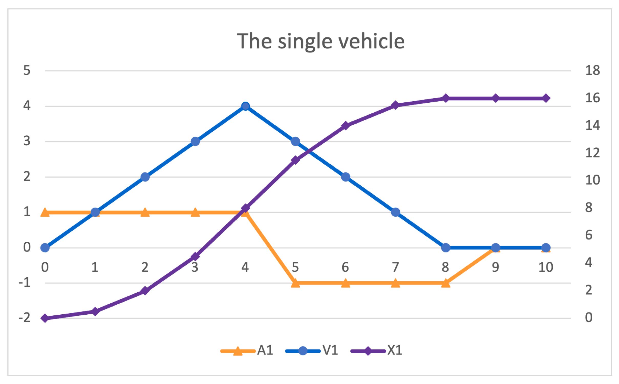
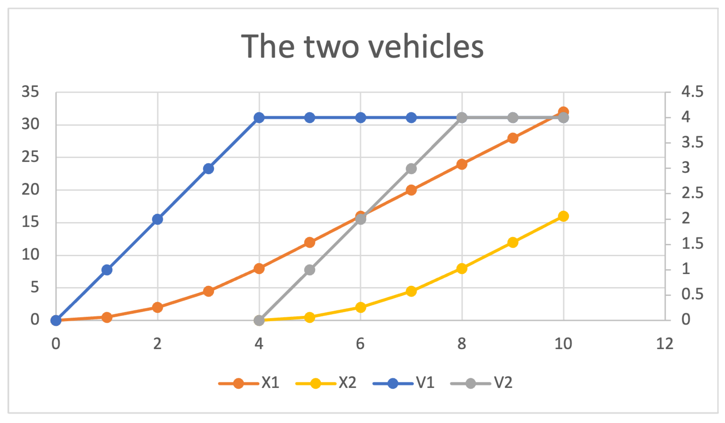
open MAINSYSTEM .
%MAINSYSTEM> red ps(tick(2,n(p2,tick(4,enter(p2,n(p1,tick(4,enter(p1,init)))
))))) .
(p1 p2):PSet
%MAINSYSTEM> red x(p1,tick(2,n(p2,tick(4,enter(p2,n(p1,tick(4,enter(p1,init)
))))))) .
(32):NzNat
%MAINSYSTEM> red v(p1,tick(2,n(p2,tick(4,enter(p2,n(p1,tick(4,enter(p1,init)
))))))) .
(4):NzNat
%MAINSYSTEM> red x(p2,tick(2,n(p2,tick(4,enter(p2,n(p1,tick(4,enter(p1,init)
))))))) .
(16):NzNat
%MAINSYSTEM> red v(p2,tick(2,n(p2,tick(4,enter(p2,n(p1,tick(4,enter(p1,init)
))))))) .
(4):NzNat
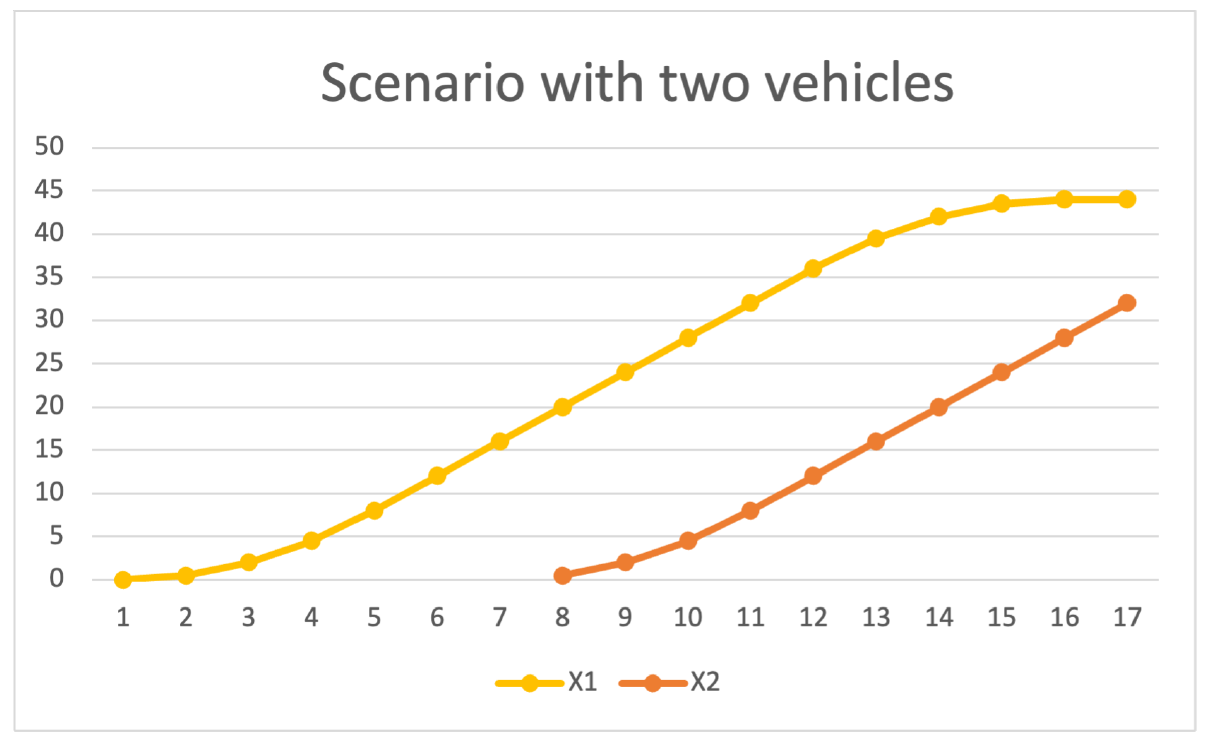
open MAINSYSTEM .
%MAINSYSTEM> red x(p1,tick(1,n(p1,tick(4,b(p1,tick(1,n(p2,tick(4,enter(p2,
tick(2,n(p1,tick(4,enter(p1,init))))))))))))) .
(44):NzNat
%MAINSYSTEM> red v(p1,tick(1,n(p1,tick(4,b(p1,tick(1,n(p2,tick(4,enter(p2,
tick(2,n(p1,tick(4,enter(p1,init))))))))))))) .
(0):Zero
%MAINSYSTEM> red x(p2,tick(1,n(p1,tick(4,b(p1,tick(1,n(p2,tick(4,enter(p2,
tick(2,n(p1,tick(4,enter(p1,init))))))))))))) .
(32):NzNat
%MAINSYSTEM> red v(p2,tick(1,n(p1,tick(4,b(p1,tick(1,n(p2,tick(4,enter(p2,
tick(2,n(p1,tick(4,enter(p1,init))))))))))))) .
(4):NzNat

%MAINSYSTEM> red c-tick(2,n(p1,tick(4,b(p1,tick(1,n(p2,tick(4,enter(p2,tick(2,
n(p1,tick(4,enter(p1,init)))))))))))) .
(false):Bool
%MAINSYSTEM> red c-tick(1,n(p1,tick(4,b(p1,tick(1,n(p2,tick(4,enter(p2,tick(2,
n(p1,tick(4,enter(p1,init)))))))))))) .
(true):Bool
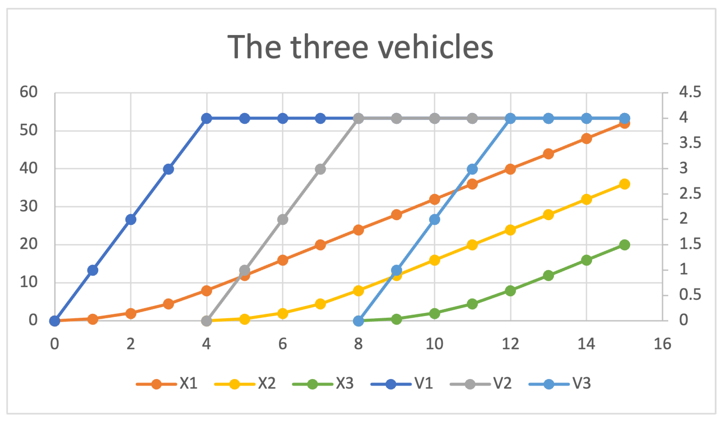
open MAINSYSTEM .
%MAINSYSTEM> red ps(tick(3,n(p3,tick(4,enter(p3,n(p2,(tick(4,enter(p2,n(p1,
tick(4,enter(p1,init)))))))))))) .
(p3 (p2 p1)):PSet
%MAINSYSTEM> red x(p1,tick(3,n(p3,tick(4,enter(p3,n(p2,(tick(4,enter(p2,n(p1,
tick(4,enter(p1,init)))))))))))) .
(52):NzNat
%MAINSYSTEM> red v(p1,tick(3,n(p3,tick(4,enter(p3,n(p2,(tick(4,enter(p2,n(p1,
tick(4,enter(p1,init)))))))))))) .
(4):NzNat
%MAINSYSTEM> red x(p2,tick(3,n(p3,tick(4,enter(p3,n(p2,(tick(4,enter(p2,n(p1,
tick(4,enter(p1,init)))))))))))) .
(36):NzNat
 %MAINSYSTEM> red v(p2,tick(3,n(p3,tick(4,enter(p3,n(p2,(tick(4,enter(p2,n(p1,
 tick(4,enter(p1,init)))))))))))) .
(4):NzNat
%MAINSYSTEM> red x(p3,tick(3,n(p3,tick(4,enter(p3,n(p2,(tick(4,enter(p2,n(p1,
tick(4,enter(p1,init)))))))))))) .
(20):NzNat
%MAINSYSTEM> red v(p3,tick(3,n(p3,tick(4,enter(p3,n(p2,(tick(4,enter(p2,n(p1,
tick(4,enter(p1,init)))))))))))) .
(4):NzNat
6.2. Model Checking
tsearch [n] t =>* p such that c in time < Twhere the bracketed number n provides an upper bound for the number of solutions to be searched and T provides an upper bound on the total duration [24,25].
6.2.1. Model Checking with Discrete Behavior
  (tsearch [1] {loc(p1,start)ps(nil)(v(p1,0)x(p1,0))} =>* {ps(p1)loc(p1,L:Label)
  v(p1,V:Rat)x(p1,X:Rat)} such that L == accel in time < 50 .)

Solution 1
L:Label --> accel ; TIME_ELAPSED:Time --> 0 ; V:Rat --> 0 ; X:Rat --> 0
- Solution 1 indicates that a state that meets the conditions is found.
- L:Label –> accel indicates that p1 has indeed entered the accel state.
- TIME_ELAPSED:Time –> 0 indicates that the state transition occurs within 0 time units (i.e., instantaneous transition).
- V:Rat –> 0 and X:Rat –> 0 indicate that when entering the accel state, p1’s velocity v(p1,0) and position x(p1,0) are still 0.
6.2.2. Model Checking with Continuous Behavior
(tsearch [1] {ps(p2 p1)loc(p2,accel)v(p2,0)x(p2,0)loc(p1,accel)v(p1,0)x(p1,9)}
=>* {ps(p2 p1)loc(p2,L2:Label)v(p2,V2:Rat)x(p2,X2:Rat)loc(p1,L1:Label)
v(p1,V1:Rat)x(p1,X1:Rat)} such that V2 > 4 in time < 50 .)
rewrites: 11040920744 in 232233443ms cpu (31227869ms real)
(47542 rewrites/second)

No solution
(tsearch [1] {ps(p2 p1)loc(p2,accel)v(p2,0)x(p2,0)loc(p1,accel)v(p1,0)x(p1,9)}
=>* {ps(p2 p1)loc(p2,L2:Label)v(p2,V2:Rat)x(p2,X2:Rat)loc(p1,L1:Label)
v(p1,V1:Rat)x(p1,X1:Rat)} such that V1 > 4 in time < 50 .)
rewrites: 11040920744 in 239387743ms cpu (32021922ms real)
(46121 rewrites/second)

No solution
(tsearch [1] {ps(p2 p1)loc(p2,accel)v(p2,0)x(p2,0)loc(p1,accel)v(p1,0)x(p1,9)}
=>* {ps(p2 p1)loc(p2,L2:Label)v(p2,V2:Rat)x(p2,X2:Rat)loc(p1,L1:Label)
v(p1,V1:Rat)x(p1,X1:Rat)} such that X2 >= X1 in time < 50 .)
rewrites: 11131793258 in 190739035ms cpu (44980131ms real)
(58361 rewrites/second)

No solution
6.2.3. Model Checking with Time Sampling
(set tick def 1/2 .)where the occurrences of 1 are replaced with .
(tsearch [1] {ps(p2 p1)loc(p2,accel)v(p2,0)x(p2,0)loc(p1,accel)v(p1,0)x(p1,9)}
=>* {ps(p2 p1)loc(p2,L2:Label)v(p2,V2:Rat)x(p2,X2:Rat)loc(p1,L1:Label)
v(p1,V1:Rat)x(p1,X1:Rat)} such that 8 > X1 - X2 in time < 20 .)
Solution 1
L2:Label --> brake ; L1:Label --> nothing ; TIME_ELAPSED:Time --> 2 ; V2:Rat
    --> 1 ; V1:Rat --> 0 ; X2:Rat --> 7/4 ; X1:Rat --> 37/4
6.2.4. Model Checking with Time Sampling 5
(set tick def 5 .)where the occurrences of 1 in the original one are replaced with 5 too. Since the time sampling is too coarse, we cannot find the situation where the distance between the rear vehicle and the front vehicle is less than 8 units as above, although there will be no collision between the two vehicles.
(tsearch [1] {ps(p2 p1)loc(p2,accel)v(p2,0)x(p2,0)loc(p1,accel)v(p1,0)x(p1,9)}
=>* {ps(p2 p1)loc(p2,L2:Label)v(p2,V2:Rat)x(p2,X2:Rat)loc(p1,L1:Label)
v(p1,V1:Rat)x(p1,X1:Rat)} such that 8 > X1 - X2 in time < 20 .)
No solution
6.3. Counterexample
eq c-tick(P2 P1,T,loc(P2,L2)v(P2,V2)x(P2,X2)loc(P1,L1)v(P1,V1)x(P1,X1)OVS) =
... (L2 = accel implies (nextx(L2,P2,T,V2,X2) + 7 < nextx(L1,P1,T,V1,X1)))
and (L2 = nothing implies (0 < nextv(L2,P2,T,V2) and nextv(L2,P2,T,V2) <= 4
and nextx(L2,P2,T,V2,X2) + 7 < nextx(L1,P1,T,V1,X1)) ...) .
(tsearch [1] {ps(p2 p1)loc(p2,accel)v(p2,0)x(p2,0)loc(p1,accel)v(p1,0)x(p1,9)}
=>* {ps(p2 p1)loc(p2,L2:Label)v(p2,V2:Rat)x(p2,X2:Rat)loc(p1,L1:Label)
v(p1,V1:Rat)x(p1,X1:Rat)} such that X2 >= X1 in time < 20 .)
Solution 1
L2:Label --> brake ; L1:Label --> nothing ; TIME_ELAPSED:Time --> 9 ; V2:Rat
    --> 0 ; V1:Rat --> 0 ; X2:Rat --> 18 ; X1:Rat --> 18
7. Conclusions
7.1. Summary of Contributions
7.2. Discussion on Model Adaptation for Real-World Features and Constraints
Author Contributions
Funding
Data Availability Statement
Conflicts of Interest
References
- Takács, D.; Zelei, A. Performance Optimization of a Formula Student Racing Car Using the IPG CarMaker, Part 1: Lap Time Convergence and Sensitivity Analysis. Eng. Proc. 2024, 79, 86. [Google Scholar] [CrossRef]
- Colley, M.; Czymmeck, J.; Kücükkocak, M.; Jansen, P.; Rukzio, E. PedSUMO: Simulacra of Automated Vehicle-Pedestrian Interaction Using SUMO To Study Large-Scale Effects. In Proceedings of the 2024 ACM/IEEE International Conference on Human-Robot Interaction, Boulder, CO, USA, 11–15 March 2024; pp. 890–895. [Google Scholar]
- Jeannin, J.B.; Ghorbal, K.; Kouskoulas, Y.; Schmidt, A.; Gardner, R.; Mitsch, S.; Platzer, A. A formally verified hybrid system for safe advisories in the next-generation airborne collision avoidance system. Int. J. Softw. Tools Technol. Transf. 2017, 19, 717–741. [Google Scholar] [CrossRef]
- Wang, Y.; Nakamura, M.; Sakakibara, K. Formal specification of an autonomous vehicle group control system with the hybrid OTS/CafeOBJ method. In Proceedings of the 2023 Congress in Computer Science, Computer Engineering, & Applied Computing (CSCE), Las Vegas, NV, USA, 24–27 July 2023; pp. 2169–2176. [Google Scholar]
- Haxthausen, A.E.; Hede, K. Formal verification of railway timetables-using the UPPAAL model checker. In From Software Engineering to Formal Methods and Tools, and Back: Essays Dedicated to Stefania Gnesi on the Occasion of Her 65th Birthday; Lecture Notes in Computer Science (LNCS, Volume 11865); Springer: Cham, Switzerland, 2019; pp. 433–448. [Google Scholar]
- Berger, U.; James, P.; Lawrence, A.; Roggenbach, M.; Seisenberger, M. Verification of the european rail traffic management system in real-time maude. Sci. Comput. Program. 2018, 154, 61–88. [Google Scholar]
- Wang, Y.; Nakamura, M.; Sakakibara, K.; Okura, Y. Formal Specification and Verification of an Autonomous Vehicle Control System by the OTS/CafeOBJ method (S). In Proceedings of the 35th International Conference on Software Engineering and Knowledge Engineering (SEKE23), Pittsburgh, PA, USA, 5–10 July 2023; pp. 363–366. [Google Scholar]
- Wang, Y.; Nakamura, M.; Sakakibara, K. Investigation of Formal Verification of the Autonomous Vehicle Control System by Specification Translation. In Proceedings of the 2023 International Technical Conference on Circuits/Systems, Computers, and Communications (ITC-CSCC), Jeju-si, Republic of Korea, 25–28 June 2023; pp. 1–6. [Google Scholar]
- Doyen, L.; Frehse, G.; Pappas, G.J.; Platzer, A. Verification of hybrid systems. In Handbook of Model Checking; Springer: Cham, Switzerland, 2018; pp. 1047–1110. [Google Scholar]
- Clavel, M.; Durán, F.; Eker, S.; Lincoln, P.; Martí-Oliet, N.; Meseguer, J.; Talcott, C. All About Maude—A High-Performance Logical Framework: How to Specify, Program and Verify Systems in Rewriting Logic; Lecture Notes in Computer Science (LNCS, Volume 4350); Springer: Berlin/Heidelberg, Germany, 2007. [Google Scholar]
- Ölveczky, P.C.; Meseguer, J. Specification and analysis of real-time systems using Real-Time Maude. In Fundamental Approaches to Software Engineering; Lecture Notes in Computer Science (LNCS, Volume 2984); Springer: Berlin/Heidelberg, Germany, 2004; pp. 354–358. [Google Scholar]
- Ölveczky, P.C.; Meseguer, J. Semantics and pragmatics of real-time Maude. High.-Order Symb. Comput. 2007, 20, 161–196. [Google Scholar]
- Ölveczky, P.C.; Meseguer, J. The real-time maude tool. In Proceedings of the International Conference on Tools and Algorithms for the Construction and Analysis of Systems, Budapest, Hungary, 29 March–6 April 2008; Springer: Berlin/Heidelberg, Germany, 2008; pp. 332–336. [Google Scholar]
- Ogata, K.; Futatsugi, K. Modeling and verification of real-time systems based on equations. Sci. Comput. Program. 2007, 66, 162–180. [Google Scholar]
- Ogata, K.; Yamagishi, D.; Seino, T.; Futatsugi, K. Modeling and verification of hybrid systems based on equations. In Design Methods and Applications for Distributed Embedded Systems; IFIP Advances in Information and Communication Technology (IFIPAICT, Volume 150); Springer: Boston, MA, USA, 2004; pp. 43–52. [Google Scholar]
- Nakamura, M.; Higashi, S.; Sakakibara, K.; Ogata, K. Specification and verification of multitask real-time systems using the OTS/CafeOBJ method. IEICE Trans. Fundam. Electron. Commun. Comput. Sci. 2022, 105, 823–832. [Google Scholar] [CrossRef]
- Diaconescu, R.; Futatsugi, K. CafeOBJ Report; World Scientific: Singapore, 1998. [Google Scholar]
- Ogata, K.; Futatsugi, K. Proof scores in the OTS/CafeOBJ method. In Formal Methods for Open Object-Based Distributed Systems, 6th IFIP WG 6.1 International Conference, FMOODS 2003, Paris, France, 19–21 November 2003; Lecture Notes in Computer Science (LNCS, Volume 2884); Springer: Berlin/Heidelberg, Germany, 2003; pp. 170–184. [Google Scholar]
- Ogata, K.; Futatsugi, K. Some tips on writing proof scores in the OTS/CafeOBJ method. In Algebra, Meaning, and Computation: Essays Dedicated to Joseph A. Goguen on the Occasion of His 65th Birthday; Springer: Berlin/Heidelberg, Germany, 2006; pp. 596–615. [Google Scholar]
- Meseguer, J. Real-Time Maude: A tool for simulating and analyzing real-time and hybrid systems. Electron. Notes Theor. Comput. Sci. 2000, 36, 361–382. [Google Scholar]
- Ölveczky, P.C.; Meseguer, J. Abstraction and completeness for real-time maude. Electron. Notes Theor. Comput. Sci. 2007, 176, 5–27. [Google Scholar]
- Ölveczky, P.C. Real-Time Maude and its applications. In Proceedings of the International Workshop on Rewriting Logic and Its Applications, Grenoble, France, 5–6 April 2014; pp. 42–79. [Google Scholar]
- Lepri, D.; Ábrahám, E.; Ölveczky, P.C. Timed CTL model checking in real-time maude. In Proceedings of the International Workshop on Rewriting Logic and Its Applications, Tallinn, Estonia, 24–25 March 2012; pp. 182–200. [Google Scholar]
- Durán, F.; Ölveczky, P.C. A guide to extending Full Maude illustrated with the implementation of Real-Time Maude. Electron. Notes Theor. Comput. Sci. 2009, 238, 83–102. [Google Scholar] [CrossRef]
- Ölveczky, P.C. Real-Time Maude 2.3 Manual. 2004. Available online: https://www.duo.uio.no/handle/10852/9834 (accessed on 2 April 2025).
- Ignatious, H.A.; Khan, M. An overview of sensors in Autonomous Vehicles. Procedia Comput. Sci. 2022, 198, 736–741. [Google Scholar]
- Rong, D.; Jin, S.; Yang, C. Connected and Autonomous Vehicle Trajectory Planning Considering Communication Delay. IEEE Trans. Veh. Technol. 2024, 73, 12668–12681. [Google Scholar]
- Yang, J.; Zhao, D.; Jiang, J.; Lan, J.; Mason, B.; Tian, D.; Li, L. A less-disturbed ecological driving strategy for connected and automated vehicles. IEEE Trans. Intell. Veh. 2023, 8, 413–424. [Google Scholar]
- Lin, Z.; Ma, J.; Duan, J.; Li, S.E.; Ma, H.; Cheng, B.; Lee, T.H. Policy iteration based approximate dynamic programming toward autonomous driving in constrained dynamic environment. IEEE Trans. Intell. Transp. Syst. 2023, 24, 5003–5013. [Google Scholar]

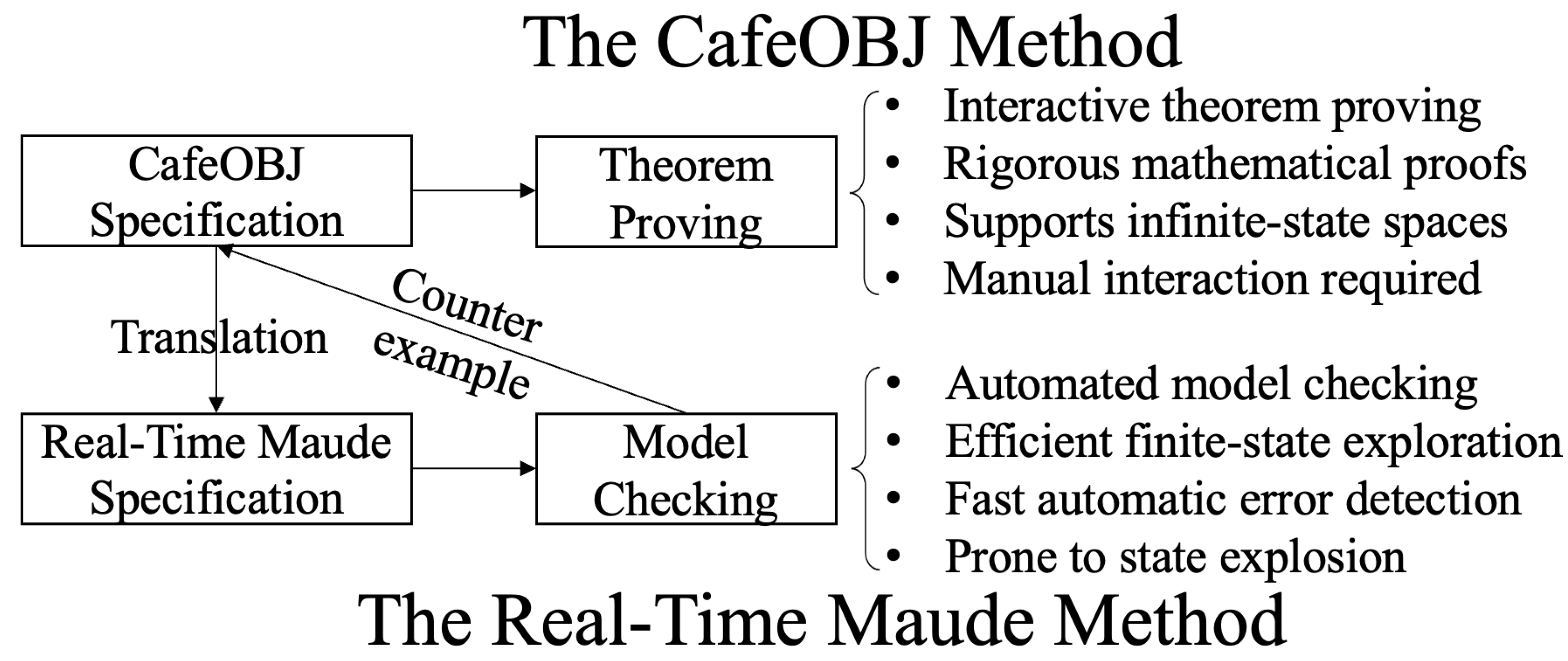
| Formal Verification | Theorem Proving | Model Checking |
|---|---|---|
| Example | CafeOBJ | Real-Time Maude |
| Advantage | infinite state spaces | fully-automated |
| Disadvantage | semi-automated | finite state spaces |
Disclaimer/Publisher’s Note: The statements, opinions and data contained in all publications are solely those of the individual author(s) and contributor(s) and not of MDPI and/or the editor(s). MDPI and/or the editor(s) disclaim responsibility for any injury to people or property resulting from any ideas, methods, instructions or products referred to in the content. |
© 2025 by the authors. Licensee MDPI, Basel, Switzerland. This article is an open access article distributed under the terms and conditions of the Creative Commons Attribution (CC BY) license (https://creativecommons.org/licenses/by/4.0/).
Share and Cite
Wang, Y.; Nakamura, M.; Takano, R.; Matsumoto, T.; Sakakibara, K. Formal Verification of Autonomous Vehicle Group Control Systems via Specification Translation of Multitask Hybrid Observational Transition Systems. Electronics 2025, 14, 1483. https://doi.org/10.3390/electronics14071483
Wang Y, Nakamura M, Takano R, Matsumoto T, Sakakibara K. Formal Verification of Autonomous Vehicle Group Control Systems via Specification Translation of Multitask Hybrid Observational Transition Systems. Electronics. 2025; 14(7):1483. https://doi.org/10.3390/electronics14071483
Chicago/Turabian StyleWang, Yifan, Masaki Nakamura, Ryo Takano, Takuya Matsumoto, and Kazutoshi Sakakibara. 2025. "Formal Verification of Autonomous Vehicle Group Control Systems via Specification Translation of Multitask Hybrid Observational Transition Systems" Electronics 14, no. 7: 1483. https://doi.org/10.3390/electronics14071483
APA StyleWang, Y., Nakamura, M., Takano, R., Matsumoto, T., & Sakakibara, K. (2025). Formal Verification of Autonomous Vehicle Group Control Systems via Specification Translation of Multitask Hybrid Observational Transition Systems. Electronics, 14(7), 1483. https://doi.org/10.3390/electronics14071483