
Applying Collaborative Co-Simulation to Railway Traction Energy Consumption

 , ,
, ,  , ,
, ,
Abstract
1. Introduction
2. Background
2.1. Energy Modeling
2.1.1. Traction Network Modeling
2.1.2. Train Power Modeling
2.2. Timetable Modeling
2.2.1. Continuous Models
2.2.2. Space-Time (Discretized) Models
2.3. Human Performance Modeling
2.4. Multi-Modeling for Systems
3. Methodology
- Rolling stock and traction power supply—Universities of Birmingham and Liverpool—Authors Z.T., X. Lyu, K.J., X. Liu
- Timetabling—Institute of Transport Studies, Leeds University—Authors Z.L., R.L.
- Rail human performance; rail signaling control—Future Mobility Group, Newcastle University—Author D.G.
- FMU integration and co-simulation—School of Computing, Newcastle University—Authors A.B., K.P.
- Setting aims—The overall aim of the project is established and shared between the project partners. Confirming our relevant areas of expertise and modeling background. Agreeing to model a linear section of track, based on the Merseyrail network with the aim of integrating:
- a.
- Timetable
- b.
- Rolling stock and power modeling
- c.
- Infrastructure models and driver models
- d.
- Integration and co-simulation
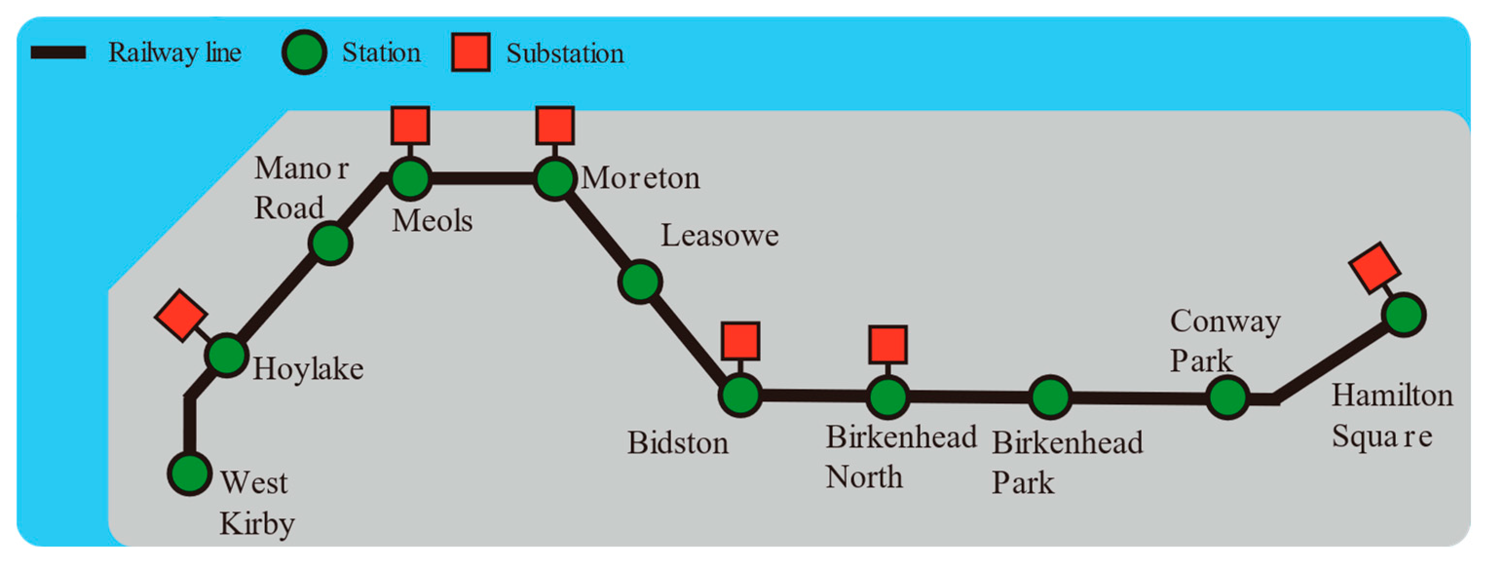
Specifically, the area of the Merseyrail network being covered was from Hamilton Square to West Kirby. This is approximately 14 km with 11 stations, including starting and terminating stations (see Figure 3).
- 2.
- Agreeing approach—In order to scope the work, a Minimum Viable Product (MVP) [52] approach was taken. This would initially involve one train running to one timetable for the specified area of infrastructure. This MVP model would then support elaboration in terms of:
- a.
- multiple timetables
- b.
- multiple trains (having more than one train running on the network at the same time and thus exploring train interactions)
- c.
- different driver profiles
- 3.
- Setting model framework—An initial architecture of models based on prior co-simulation work [9].
- 4.
- Develop timetable—A timetable needed to be generated for the Merseyrail network from Leeds University. A number of variants of the timetable were then generated with different headways.
- 5.
- Tuning the baseline—Integrating the Merseyrail infrastructure (signaling, track distance, speed limits, stations) information and the Leeds-generated timetable into the pre-existing co-simulation from [41].
- 6.
- FMU of rolling stock and power model—Replacing the pre-existing rolling stock and power models from ANNSIM with the more accurate combined rolling stock and power model from Birmingham University.
- 7.
- Running co-simulations—Taking adapted models and running them to generate power outputs. Running co-simulation in different scenarios (timetable variants, multiple trains, and driver variants).
- 8.
- Display outputs—using co-simulation outputs to calculate energy consumption for different simulation scenarios.
4. Base Models
4.1. Initial Rail Infrastructure and Driver Models
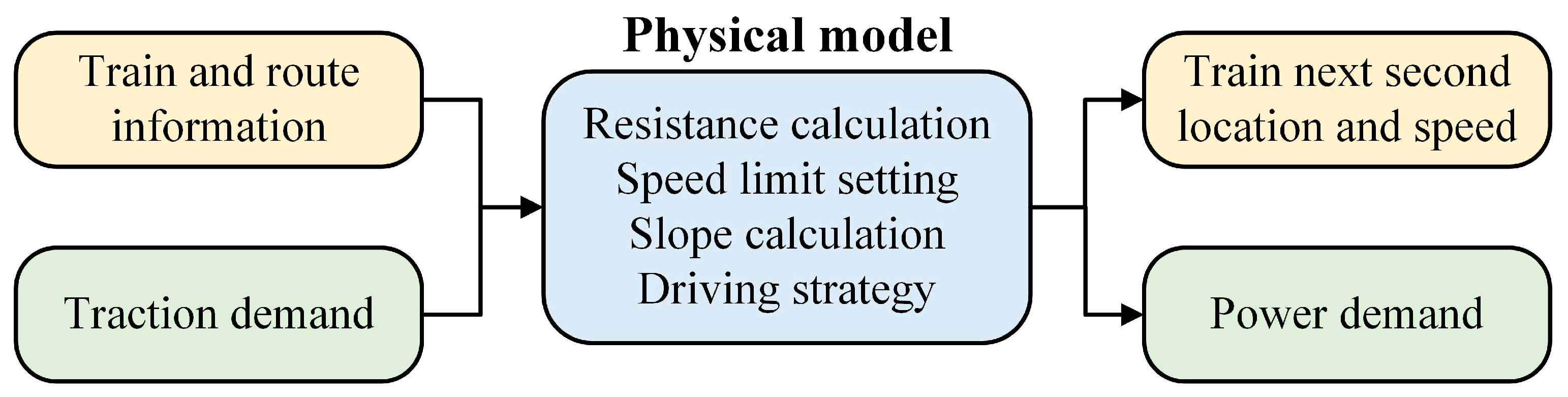
4.2. Traction Power Model
4.3. Timetable Model
Generating the Timetable for the Use Case Context
5. Results
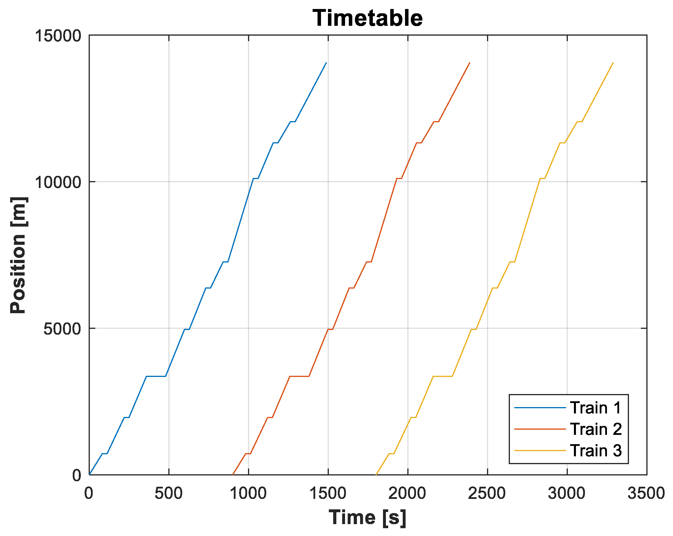
5.1. Timetable Outputs
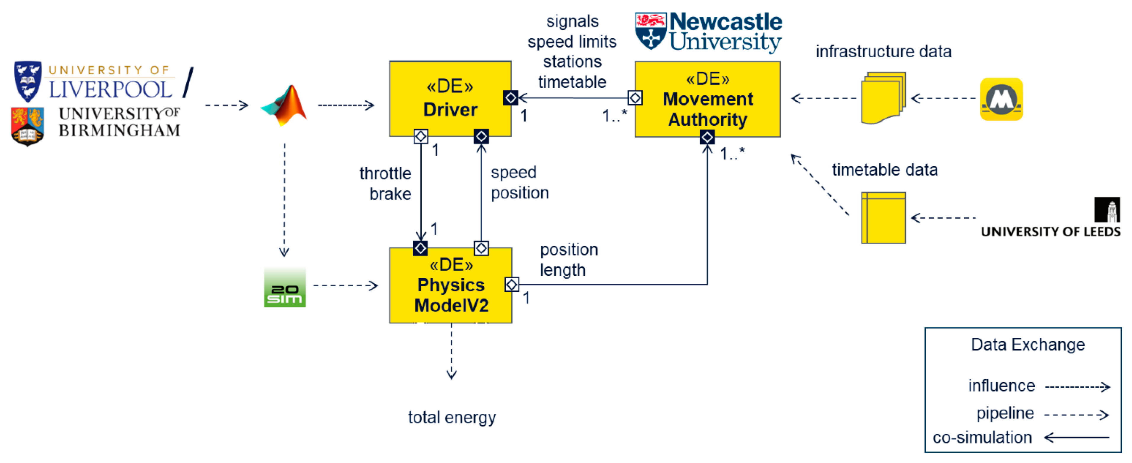
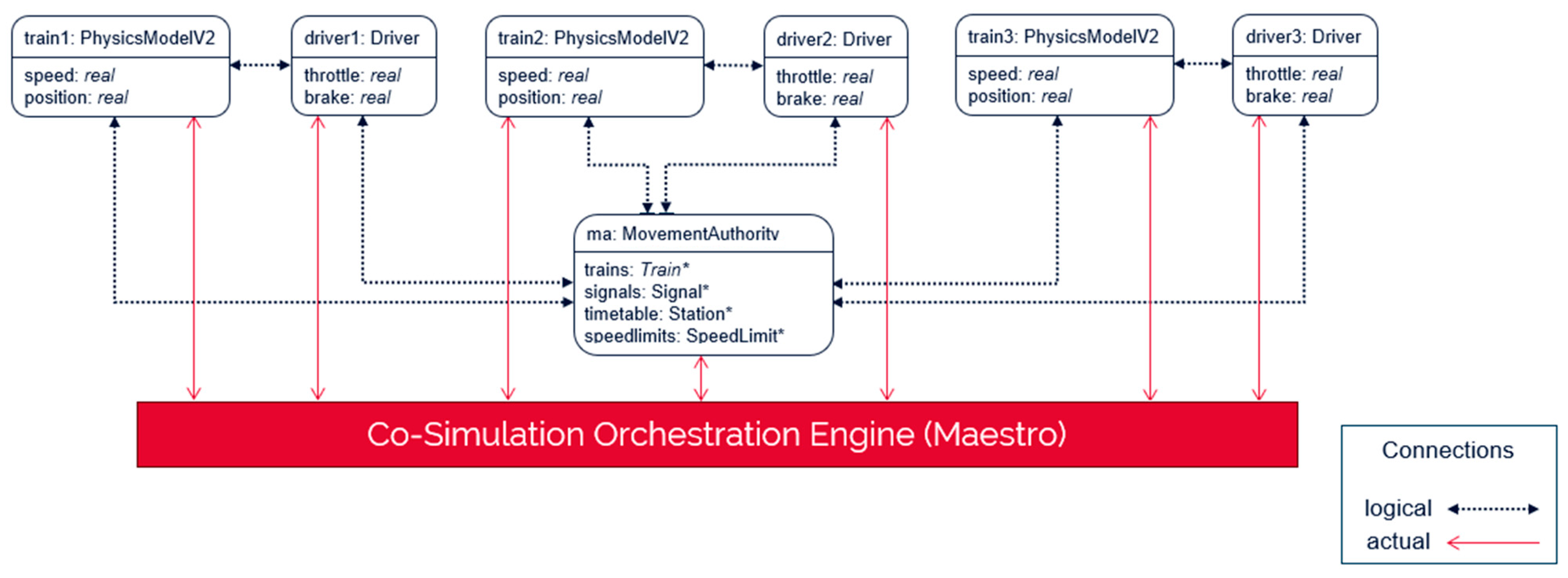
5.2. Integrated System Model
5.3. Co-Simulation Outputs
- Graph 1: Position—Here, we see a train moving from 0 m (at rest) to ≈2000 m. The train stops at two stations along the way.
- Graph 2: Next Signal—This shows the signal the driver sees, in this case, a value of 5 that indicates a green aspect.
- Graph 3: Speed—This is the speed of the train (m/s). The train comes up to speed and slows to a stop for each station. Notice the line speed restriction in the first few seconds of the co-simulation.
- Graph 4: Throttle/Brake Set Points—This shows the notched throttle and brake outputs between 0 and 1. Notice there is some oscillation as the algorithm of the driver is discrete-event and acts similarly to a PWM signal to ensure the train stops at the right point and time.
- Graph 5: Energy/Power Draw—This shows the cumulative energy used by the train during the run.
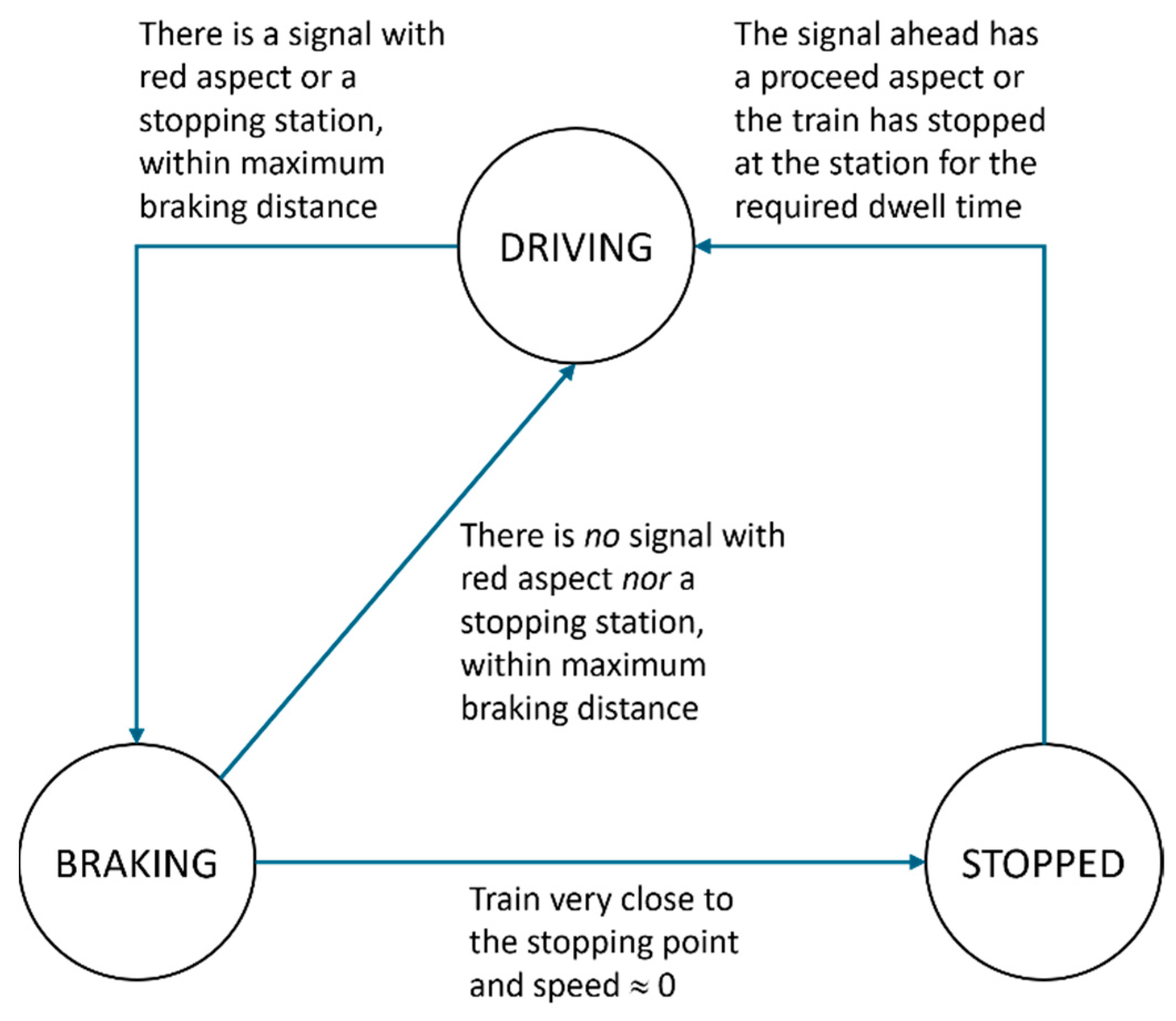
- Graph 6: Move State/Driving State—This is an indication of which mode the driver is in, as seen in Figure 5 (STOPPED, BRAKING, DRIVING).
6. Discussion
6.1. Discussion of Outputs
6.2. Model Development and Integration
6.3. Collaboration
6.4. Limitations
7. Conclusions
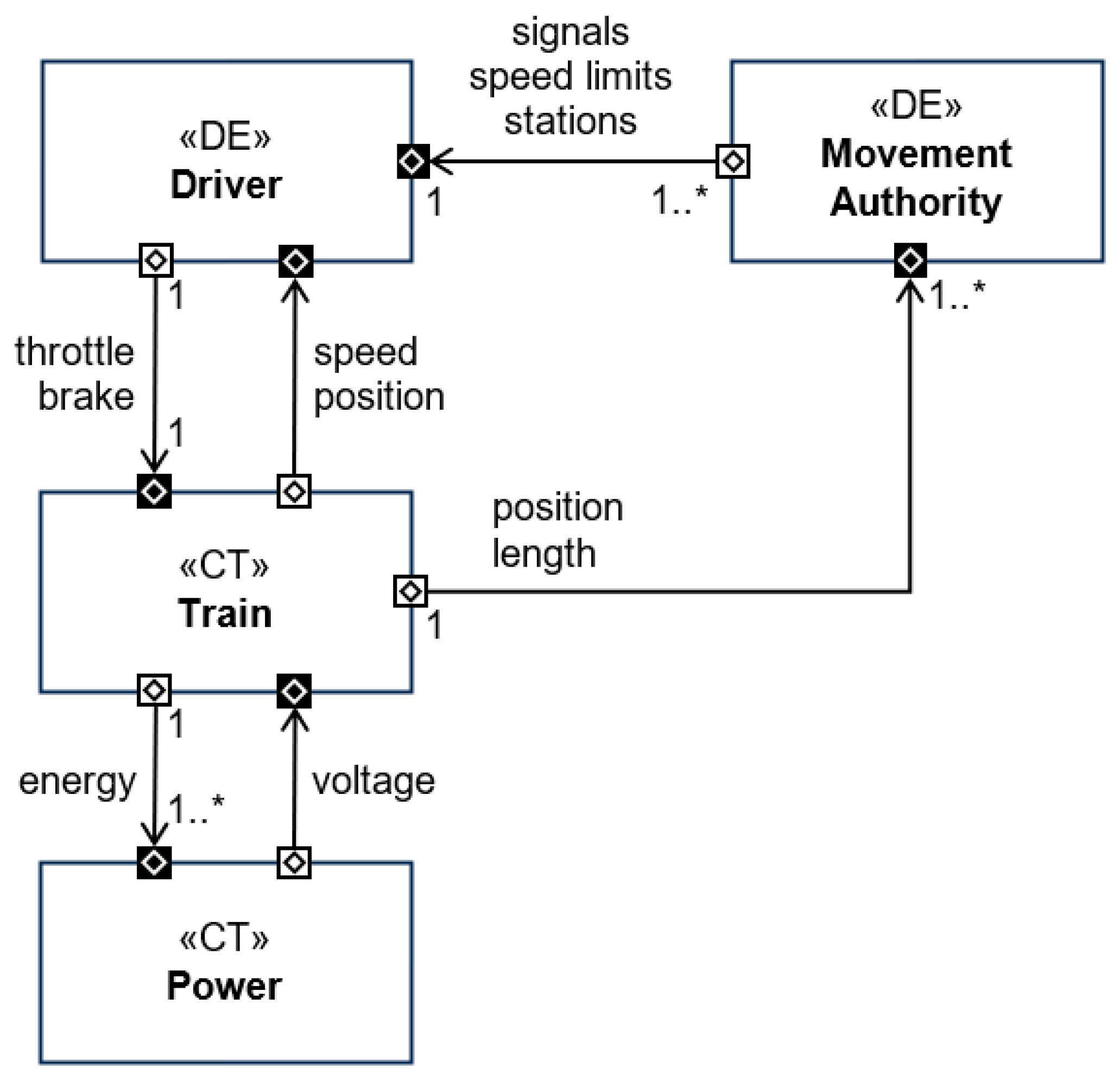
- a control element (how the driver inputs control actions to the train model), and
- a behavioral element (how the driver processes and reacts to information from the infrastructure; the policy for implementing control actions such as driving under yellow aspects or managing station arrival times)
Author Contributions
Funding
Data Availability Statement
Conflicts of Interest
Glossary
| Notation | Meaning |
| A | Acceleration of train (m/s2) |
| F | Traction force of train (N) |
| g | Gravitational acceleration (m/s2) |
| M | Mass of train (kg) |
| P | Power draw of train (W) |
| R | Total resistance to motion of train (N) |
| t | Time (s) |
| speed | Current speed of train (m/s) |
| Slope angle | |
| dist_to_stop | Distance from current position to next stopping point |
| reqd_speed | Speed required at the start of braking to stop the train at the correct time |
| duration_to_stop | Duration between the current time and the time when the train is required to stop |
| K | Ratio of the maximum power draw of the train to the mass of the train |
| gear | Gear value in the closed interval [−1, 1] with gear > 0 denoting acceleration and gear < 0 denoting deceleration |
| Trains and in the set of trains | |
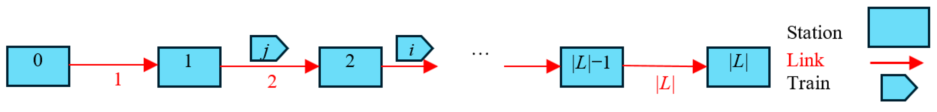
| Link in the set of links | |
| |L| | The number of links |
| Time at which train enters link , and thereby departs from station − 1 | |
| Time at which train leaves link , and thereby arrives at station | |
| Decision variable on whether or not train immediately precedes train on link | |
| , | Artificially introduced first and last dummy trains on link |
| H | Duration parameters such as headway and dwell time in train timetabling, including variants such as |
| Minimum time required for train to travel across link | |
| Minimum waiting time required for train at station | |
| Minimum departure-departure headway between trains and at station − 1 | |
| Minimum arrival-arrival headway between trains and at station |
References
- Ceraolo, M.; Lutzemberger, G.; Frilli, A.; Pugi, L. Regenerative Braking in High Speed Railway Applications: Analysis by Different Simulation Tools. In Proceedings of the 2016 IEEE 16th International Conference on Environment and Electrical Engineering (EEEIC), Florence, Italy, 7–10 June 2016; IEEE: Piscataway, NJ, USA, 2016; pp. 1–5. [Google Scholar]
- Arboleya, P.; Mayet, C.; Mohamed, B.; Aguado, A.J.; de la Torre, S. A review of railway feeding infrastructures: Mathematical models for planning and operation. eTransportation 2020, 5, 100063. [Google Scholar]
- Hoffrichter, A.; Silmon, J.; Schmid, F.; Hillmansen, S.; Roberts, C. Feasibility of discontinuous electrification on the Great Western Main Line determined by train simulation. Proc. Inst. Mech. Eng. Part F J. Rail Rapid Transit 2013, 227, 296–306. [Google Scholar]
- Abdurahman, B.M.; Harrison, T.; Ward, C.P.; Midgley, W.J. An investigation into intermittent electrification strategies and an analysis of resulting CO2 emissions using a high-fidelity train model. Railw. Eng. Sci. 2021, 29, 314–326. [Google Scholar]
- Chen, M.; Feng, X.; Guo, Y.; Tao, X.; Sun, P.; Wang, Q. Optimal Cooperative Eco-Driving of Multitrain with TLET Comprehensive System. IEEE Trans. Transp. Electrif. 2024, 10, 2095–2111. [Google Scholar]
- González-Gil, A.; Palacin, R.; Batty, P.; Powell, J.P. A systems approach to reduce urban rail energy consumption. Energy Convers. Manag. 2014, 80, 509–524. [Google Scholar]
- Chen, L.; James, P.; Kirkwood, D.; Nguyen, H.N.; Nicholson, G.L.; Roggenbach, M. Towards Integrated Simulation and formal Verification of Rail Yard Designs—An Experience Report Based on the UK East Coast Main Line. In Proceedings of the 2016 IEEE International Conference on Intelligent Rail Transportation (ICIRT), Birmingham, UK, 23–25 August 2016; IEEE: Piscataway, NJ, USA, 2016; pp. 347–355. [Google Scholar]
- Winnett, J.; Iraklis, A.; Keating, E.; McGordon, A.; Ridler, T.; Hughes, D.J. Automotive to Rail: Can Technologies Cross the Gap? In Proceedings of the Stephenson Conference: Research for Railways 2017, London, UK, 25–27 April 2017; Institute of Mechanical Engineers: London, UK, 2017; pp. 529–538. [Google Scholar]
- Golightly, D.; Pierce, K.; Palacin, R.; Gamble, C. A feasibility assessment of multi-modelling approaches for rail decarbonisation systems simulation. Proc. Inst. Mech. Eng. Part F J. Rail Rapid Transit 2022, 236, 715–732. [Google Scholar]
- Harrison, T.J.; Midgley, W.J.; Goodall, R.M.; Ward, C.P. Development and control of a rail vehicle model to reduce energy consumption and carbon dioxide emissions. Proc. Inst. Mech. Eng. Part F J. Rail Rapid Transit 2021, 235, 1237–1248. [Google Scholar]
- Thule, C.; Lausdahl, K.; Gomes, C.; Meisl, G.; Larsen, P.G. Maestro: The INTO-CPS co-simulation framework. Simul. Model. Pract. Theory 2019, 92, 45–61. [Google Scholar]
- Abbiati, G.; Baş, E.E.; Gomes, C.; Larsen, P.G. Hybrid fire testing using FMI-based co-simulation. Fire Saf. J. 2023, 139, 103832. [Google Scholar]
- Shao, X.; Ringsberg, J.W.; Johnson, E.; Li, Z.; Yao, H.D.; Skjoldhammer, J.G.; Björklund, S. An FMI-based co-simulation framework for simulations of wave energy converter systems. Energy Convers. Manag. 2025, 323, 119220. [Google Scholar]
- Yuan, W.; Frey, H.C. Potential for metro rail energy savings and emissions reduction via eco-driving. Appl. Energy 2020, 268, 114944. [Google Scholar]
- Bader, M.P.; Lobyntsev, V.V. Increasing the Energy Efficiency of DC Traction Power Supply Systems. Russ. Electr. Eng. 2020, 9, 541–545. [Google Scholar] [CrossRef]
- Dong, H.; Tian, Z.; Spencer, J.W.; Fletcher, D.; Hajiabady, S. Bilevel Optimization of Sizing and Control Strategy of Hybrid Energy Storage System in Urban Rail Transit Considering Substation Operation Stability. IEEE Trans. Transp. Electrif. 2024, 10, 10102–10114. [Google Scholar]
- Tian, Z.; Weston, P.; Zhao, N.; Hillmansen, S.; Roberts, C.; Chen, L. System energy optimisation strategies for metros with regeneration. Transp. Res. Part C Emerg. Technol. 2017, 75, 120–135. [Google Scholar]
- Tian, Z.; Zhao, N.; Hillmansen, S.; Roberts, C.; Dowens, T.; Kerr, C. SmartDrive: Traction energy optimization and applications in rail systems. IEEE Trans. Intell. Transp. Syst. 2019, 20, 2764–2773. [Google Scholar]
- Jiang, K.; Tian, Z.; Wen, T.; Hillmansen, S.; Zhang, Y. Cost modelling-based route applicability analysis of United Kingdom passenger railway decarbonisation options. Int. J. Electr. Power Energy Syst. 2024, 160, 110094. [Google Scholar]
- Medeossi, G.; de Fabris, S. Simulation of Rail Operations. In Handbook of Optimization in the Railway Industry; Springer International Publishing: Berlin/Heidelberg, Germany, 2018; pp. 1–24. [Google Scholar]
- Szpigel, B. Optimal train scheduling on a single track railway. Oper. Res. 1973, 72, 343–351. [Google Scholar]
- Carey, M.; Lockwood, D. A model, algorithms and strategy for train pathing. J. Oper. Res. Soc. 1995, 46, 988–1005. [Google Scholar]
- Higgins, A.; Kozan, E.; Ferreira, L. Optimal scheduling of trains on a single line track. Transp. Res. Part B Methodol. 1996, 30, 147–161. [Google Scholar]
- Cordeau, J.F.; Toth, P.; Vigo, D. A survey of optimization models for train routing and scheduling. Transp. Sci. 1998, 32, 380–404. [Google Scholar]
- Kroon, L.G.; Peeters, L.W. A variable trip time model for cyclic railway timetabling. Transp. Sci. 2003, 37, 198–212. [Google Scholar]
- Kroon, L.G.; Dekker, R.; Vromans, M.J. Cyclic Railway Timetabling: A Stochastic Optimization Approach. In Algorithmic Methods for Railway Optimization: International Dagstuhl Workshop, Dagstuhl Castle, Germany, 20–25 June, 2004, 4th International Workshop, ATMOS 2004, Bergen, Norway, 16–17 September 2004; Revised Selected Papers; Springer: Berlin/Heidelberg, Germany, 2007; pp. 41–66. [Google Scholar]
- Meng, L.; Zhou, X. Robust single-track train dispatching model under a dynamic and stochastic environment: A scenario-based rolling horizon solution approach. Transp. Res. Part B Methodol. 2011, 45, 1080–1102. [Google Scholar]
- Caprara, A.; Fischetti, M.; Toth, P. Modeling and Solving the Train Timetabling Problem. Oper. Res. 2002, 50, 851–861. [Google Scholar] [CrossRef]
- Cacchiani, V.; Toth, P. Nominal and robust train timetabling problems. Eur. J. Oper. Res. 2012, 219, 727–737. [Google Scholar] [CrossRef]
- Fang, W.; Yang, S.; Yao, X. A survey on problem models and solution approaches to rescheduling in railway networks. IEEE Trans. Intell. Transp. Syst. 2015, 16, 2997–3016. [Google Scholar]
- Ellis, R.; Weston, P.; Stewart, E.; Hillmansen, S.; Tricoli, P.; Roberts, C.; Jones, I. Observations of train control performance on a camshaft-operated DC electrical multiple unit. Proc. Inst. Mech. Eng. Part F J. Rail Rapid Transit 2016, 230, 1184–1201. [Google Scholar]
- Luijt, R.S.; van den Berge, M.P.; Willeboordse, H.Y.; Hoogenraad, J.H. 5 years of Dutch eco-driving: Managing behavioural change. Transp. Res. Part A Policy Pract. 2017, 98, 46–63. [Google Scholar]
- Naweed, A. Investigations into the skills of modern and traditional train driving. Appl. Ergon. 2014, 45, 462–470. [Google Scholar]
- Burggraaf, J.; Groeneweg, J.; Sillem, S.; van Gelder, P. What employees do today because of their experience yesterday: How incidental learning influences train driver behavior and safety margins (a big data analysis). Safety 2021, 7, 2. [Google Scholar] [CrossRef]
- Filtness, A.J.; Naweed, A. Causes, consequences and countermeasures to driver fatigue in the rail industry: The train driver perspective. Appl. Ergon. 2017, 60, 12–21. [Google Scholar] [PubMed]
- Balfe, N.; Crowley, K.; Smith, B.; Longo, L. Estimation of Train Driver Workload: Extracting Taskload Measures from On-Train-Data-Recorders. In Human Mental Workload: Models and Applications: First International Symposium, H-WORKLOAD 2017, Dublin, Ireland, 28–30 June 2017; Revised Selected Papers 1; Springer International Publishing: Berlin/Heidelberg, Germany, 2017; pp. 106–119. [Google Scholar]
- Al-Mekhlafi, A.B.A.; Isha, A.S.N.; Chileshe, N.; Abdulrab, M.; Saeed, A.A.H.; Kineber, A.F. Modelling the relationship between the nature of work factors and driving performance mediating by role of fatigue. Int. J. Environ. Res. Public Health 2021, 18, 6752. [Google Scholar] [CrossRef] [PubMed]
- Hamilton, W.I.; Clarke, T. Driver Performance Modelling and its Practical Application to Railway Safety. In Rail Human Factors; Routledge: Oxfordshire, UK, 2017; pp. 25–39. [Google Scholar]
- Nneji, V.C.; Cummings, M.L.; Stimpson, A.J. Predicting locomotive crew performance in rail operations with human and automation assistance. IEEE Trans. Hum. Mach. Syst. 2019, 49, 250–258. [Google Scholar]
- Golightly, D.; Gamble, C.; Palacin, R.; Pierce, K. Applying ergonomics within the multi-modelling paradigm with an example from multiple UAV control. Ergonomics 2020, 63, 1027–1043. [Google Scholar] [PubMed]
- Pierce, K.; Bhattacharyya, A.; Golightly, D.; da Silva, P.P.; Merricks, S.; Palacin, R.; Guo, Z. Using Co-Simulation and Time Signal at Red (TSAR) to Determine Impact of Driver Behavior on Rail Network Performance. In Proceedings of the 2024 Annual Modeling and Simulation Conference (ANNSIM), Washington, DC, USA, 20–23 May 2024; IEEE: Piscataway, NJ, USA, 2024; pp. 1–13. [Google Scholar]
- Available online: https://github.com/nickbattle/vdmj (accessed on 19 January 2025).
- Available online: https://overturetool.org/ (accessed on 19 January 2025).
- Broenink, J.F. Modelling, simulation and analysis with 20-sim. J. A 1997, 38, 22–25. [Google Scholar]
- Blochwitz, T.; Otter, M.; Åkesson, J.; Arnold, M.; Clauss, C.; Elmqvist, H.; Friedrich, M.; Junghanns, A.; Mauss, J.; Neumerkel, D.; et al. Functional mockup interface 2.0: The standard for tool independent exchange of simulation models. In Proceedings of the 9th International MODELICA Conference, Munich, Germany, 3–5 September 2012; pp. 173–184. [Google Scholar]
- Available online: https://into-cps.org/ (accessed on 19 January 2025).
- Foldager, F.F.; Larsen, P.G.; Green, O. Development of a Driverless Lawn Mower Using Co-Simulation. In Software Engineering and Formal Methods: SEFM 2017 Collocated Workshops: DataMod, FAACS, MSE, CoSim-CPS, and FOCLASA, Trento, Italy, 4–5 September 2017; Revised Selected Papers 15; Springer International Publishing: Berlin/Heidelberg, Germany, 2018; pp. 330–344. [Google Scholar]
- Neghina, M.; Zamfirescu, C.B.; Pierce, K. Early-stage analysis of cyber-physical production systems through collaborative modelling. Softw. Syst. Model. 2020, 19, 581–600. [Google Scholar]
- Zamfirescu, C.B.; Neghină, M. Collaborative development of a CPS-based production system. Procedia Comput. Sci. 2019, 162, 579–586. [Google Scholar]
- Pieper, T.; Obermaisser, R. Distributed Co-Simulation for Software-in-the-Loop Testing of Networked Railway Systems. In Proceedings of the 2018 7th Mediterranean Conference on Embedded Computing (MECO), Budva, Montenegro, 10–14 June 2018; IEEE: Piscataway, NJ, USA, 2018; pp. 1–5. [Google Scholar]
- Kugu, O.; Zhou, S.; Nowak, R.; Müller, G.; Reiterer, S.H.; Meierhofer, A.; Grafinger, M. An FMI-and SSP-based Model Integration Methodology for a Digital Twin Platform of a Holistic Railway Infrastructure System. In Proceedings of the Modelica Conferences, Aachen, Germany, 9–11 October 2023; pp. 717–726. [Google Scholar]
- Stevenson, R.; Burnell, D.; Fisher, G. The Minimum Viable Product (MVP): Theory and Practice. J. Manag. 2024, 50, 01492063241227154. [Google Scholar]
- Haith, J.; Johnson, D.; Nash, C. The case for space: The measurement of capacity utilisation, its relationship with reactionary delay and the calculation of the capacity charge for the British rail network. Transp. Plan. Technol. 2014, 37, 20–37. [Google Scholar]
- Powell, J.P.; Palacin, R. A comparison of modelled and real-life driving profiles for the simulation of railway vehicle operation. Transp. Plan. Technol. 2015, 38, 78–93. [Google Scholar]
- Lomonossoff, G.V. Introduction to Railway Mechanics; Oxford University Press: Oxford, UK, 1933. [Google Scholar]
- Lusby, R.M.; Larsen, J.; Ehrgott, M.; Pisinger, D. Railway track allocation: Models and methods. OR Spectr. 2011, 33, 843–883. [Google Scholar]


| Station | Location (km) | Dwelling Time (s) | Running Time (s) | Link Index |
|---|---|---|---|---|
| Hamilton Square | 0 | - | - | - |
| Conway Park | 0.72 | 30 | 90 | 1 |
| Birkenhead Park | 1.95 | 30 | 120 | 2 |
| Birkenhead North | 3.36 | 120 | 120 | 3 |
| Biston | 4.96 | 30 | 120 | 4 |
| Leasowe | 6.37 | 30 | 120 | 5 |
| Moreton | 7.26 | 30 | 90 | 6 |
| Meols | 10.11 | 30 | 155 | 7 |
| Manor Road | 11.32 | 30 | 120 | 8 |
| Hoylake | 12.04 | 30 | 90 | 9 |
| West Kirby | 14.06 | - | 300 | 10 |
| Energy Consumption (Kilo Watt Hours) | 25% Time Margin | |
|---|---|---|
| Headway 600 s (10 min) | Headway 300 s (5 min) | |
| Baseline 1 | 66.2809 | 66.2809 |
| Baseline 2 | 66.2808 | 66.9367 |
| Baseline 3 | 66.2808 | 68.6789 |
| Defensive 1 | 66.2880 | 66.2880 |
| Defensive 2 | 66.2741 | 68.0183 |
| Defensive 3 | 66.2741 | 68.0183 |
| Baseline Total | 198.84 | 201.90 |
| Defensive Total | 198.84 | 202.32 |
Disclaimer/Publisher’s Note: The statements, opinions and data contained in all publications are solely those of the individual author(s) and contributor(s) and not of MDPI and/or the editor(s). MDPI and/or the editor(s) disclaim responsibility for any injury to people or property resulting from any ideas, methods, instructions or products referred to in the content. |
© 2025 by the authors. Licensee MDPI, Basel, Switzerland. This article is an open access article distributed under the terms and conditions of the Creative Commons Attribution (CC BY) license (https://creativecommons.org/licenses/by/4.0/).
Share and Cite
Golightly, D.; Bhattacharyya, A.; Pierce, K.; Tian, Z.; Lin, Z.; Liu, R.; Lyu, X.; Jiang, K.; Liu, X. Applying Collaborative Co-Simulation to Railway Traction Energy Consumption. Electronics 2025, 14, 1467. https://doi.org/10.3390/electronics14071467
Golightly D, Bhattacharyya A, Pierce K, Tian Z, Lin Z, Liu R, Lyu X, Jiang K, Liu X. Applying Collaborative Co-Simulation to Railway Traction Energy Consumption. Electronics. 2025; 14(7):1467. https://doi.org/10.3390/electronics14071467
Chicago/Turabian StyleGolightly, David, Anirban Bhattacharyya, Ken Pierce, Zhongbei Tian, Zhiyuan Lin, Ronghui Liu, Xinnan Lyu, Kangrui Jiang, and Xiao Liu. 2025. "Applying Collaborative Co-Simulation to Railway Traction Energy Consumption" Electronics 14, no. 7: 1467. https://doi.org/10.3390/electronics14071467
APA StyleGolightly, D., Bhattacharyya, A., Pierce, K., Tian, Z., Lin, Z., Liu, R., Lyu, X., Jiang, K., & Liu, X. (2025). Applying Collaborative Co-Simulation to Railway Traction Energy Consumption. Electronics, 14(7), 1467. https://doi.org/10.3390/electronics14071467