Geographic Routing Decision Method for Flying Ad Hoc Networks Based on Mobile Prediction

Abstract

Flying ad hoc networks (FANETs) have highly dynamic and energy-limited characteristics. Compared with traditional mobile ad hoc networks, their nodes move faster and their topology changes more frequently. Therefore, the design of routing protocols faces greater challenges. The existing routing schemes rely on frequent and fixed-interval Hello transmissions, which exacerbates network load and leads to high communication energy consumption and outdated location information. MP-QGRD combined with the extended Kalman filter (EKF) is used for node position prediction, and the Hello packet transmission interval is dynamically adjusted to optimize neighbor discovery. At the same time, reinforcement learning methods are used to comprehensively consider link stability, energy consumption, and communication distance for routing decisions. The simulation results show that compared to QMR, QGeo, and GPSR, MP-QGRD has an increased packet delivery rate, end-to-end latency, and communication energy consumption by 10%, 30%, and 15%, respectively.

1. Introduction

In recent years, unmanned aerial vehicles (UAVs) have been widely used in military and civilian fields, ushering in a new development stage [1]. Flying ad hoc networks (FANET) [2] have emerged as a unique wireless communication network construction method, demonstrating enormous potential. FANETs can achieve self-organizing network construction of flight nodes without pre-establishing a static network, with flexible node deployment, rapid networking capabilities, strong adaptability, and easy implementation characteristics [3].

However, the high-speed mobility and high energy consumption of flying nodes also bring about a series of severe challenges [4]. The high-speed movement of UAVs’ nodes leads to continuous variations in network topology and frequent link interruptions, further resulting in increased uncertainty and latency in data transmission [5]. Existing works generally have the problem of high-frequency routing detection consumption [6], especially the frequent sending of Hello packets in fixed time slots [7,8], which leads to large communication energy consumption and wireless link congestion [9]. At the same time, the fixed exploration mode lags behind the position perception of neighbor nodes, which affects the accuracy of routing. Some studies [10,11] indicate that, in FANET, frequent long-distance communication will significantly affect the overall energy consumption of UAVs, and unbalanced energy consumption may lead to the failure of routing paths, thus shortening network stability.

In order to solve the problem of energy limitation, this article integrates the motion information and remaining energy level of UAVs into the routing process to balance communication and flight requirements [12], thereby avoiding excessive energy consumption and network instability. Considering the relationship between energy consumption and flight stability, the routing decision maximizes network stability while ensuring communication quality by reasonably predicting the motion trajectory and energy state of nodes [13].

To address the issues of frequent link interruptions and high energy consumption caused by the frequent changes in node position in FANETs, this paper proposes a carefully designed routing protocol, divided into three key components: mobile prediction, neighbor discovery, and routing decision. Neighbor mobile prediction can accurately perceive the flight status of neighboring nodes and dynamically adjust the Hello packet sending gap. Adopting reinforcement learning methods [14], routing decisions are made by comprehensively considering link stability, communication energy consumption, and distance factors [15]. This innovative design enables better adaptation to the environment of frequent node position changes and makes more accurate and intelligent decisions. The contributions of this paper are as follows:

• By introducing the extended Kalman filter (EKF) prediction model [16], the prediction of node positions in flying ad hoc networks has been achieved, reducing the problem of position failure caused by the high dynamics of nodes in the time slot interval of position detection.
• Designing a mechanism for dynamically adjusting the Hello packet sending gap, optimizing the neighbor discovery process, reducing the neighbor discovery requirements of high-speed mobile nodes, and significantly reducing routing detection overhead.
• Introducing a Q-learning algorithm with adaptive adjustment of the learning rate and discount factor for intelligent routing decision-making. Taking into account link stability, energy, and distance metrics, a reward function is designed to maximize the reward for routing decisions, thereby improving network performance and stability.

The remaining structure of this paper is as follows: In Section 2, related work on routing protocols for current FANETs is summarized. Section 3 introduces the network model, and provides the design and performance analysis of the MP-QGRD algorithm. In Section 4, the experimental results are presented and analyzed. Section 5 provides a summary of the work presented in this paper.

2. Related Work

Many researchers have delved into the routing decision methods for MANETs and have achieved fruitful research results. The existing work can be roughly divided into reactive routing, proactive routing, and geographic routing [17]. The following is our analysis and summary.

2.1. Reactive Routing

Reactive routing is an on-demand routing mechanism where nodes do not actively maintain routing information but instead discover paths through flooding control messages when data transmission is needed, thereby saving computational resources and communication traffic. The advantage of this method is that it reduces network overhead, but it also brings higher route discovery latency.

AODV (Ad hoc on-demand distance vector) [18] is a classic representative of reactive routing protocols. It discovers neighboring nodes by sending Hello packets in fixed time slots, but when communicating with the target node, it must perform a route discovery process to find a path. To improve the efficiency of route discovery and reduce latency, Bai et al. proposed a method called DOA (DSR over AODV) [19] that combines AODV and DSR (dynamic source routing). This method uses AODV for reactive routing within clusters and DSR for maintaining a complete routing table between clusters. This scheme combines the advantages of two protocols, but still has certain limitations in complex network environments.

Most reactive routing protocols do not fully consider the issues of multi-path selection and optimal path selection. To this end, Wang et al. [20] proposed the AO-AOMDV (arithmetic optimization ad hoc on-demand multi-path distance vector ) protocol, which enhances the effectiveness of multi-path routing protocols through arithmetic optimization to reduce latency during data transmission. However, the protocol still faces high latency in route discovery and poor link stability in high dynamic environments. To further improve the quality of path selection, Sarkar et al. [21] proposed the Enhanced-Ant-AODV protocol, which uses the ant colony algorithm to comprehensively consider factors such as node reliability, congestion, hop count, and remaining energy to optimize routing selection and improve service quality. However, in high dynamic scenarios, the fixed Hello packet mechanism still struggles to adapt to rapidly changing network environments. In addition, routing protocols based on natural heuristic algorithms have slow convergence speeds and face issues such as increased latency, high communication overhead, and energy consumption.

Unbalanced energy consumption may lead to the failure of routing paths, thereby shortening network stability. The ECaD (energy-efficient connected aware data transmission) scheme [10] attempts to reduce energy consumption by prioritizing the selection of high-energy nodes for route discovery. Joon et al. [22] introduced the Q-learning algorithm EAQ-AODV (energy-aware Q-learning ad hoc on-demand distance vector), which selects cluster head nodes through a reward mechanism and dynamically adjusts routing strategies based on environmental changes and historical experience to optimize the routing process and reduce energy consumption.

2.2. Proactive Routing

The proactive routing protocol [23] maintains the global topology through regular information exchange between nodes. Nodes not only discover neighbors by sending Hello packets but also exchange routing information to perceive real-time changes in network topology. The advantage of this method is that it can reduce the delay during route discovery.

Islam et al. [24] proposed using a combination of graph neural networks and software defined networks to optimize routing selection in the network through the learning ability of graph neural networks in order to meet the transmission needs of different types of data packets. However, since FANET has higher mobility than ordinary ad hoc networks, Gangopadhyay et al. [25] proposed an improved OLSR (optimized link state routing) protocol based on UAV residual energy and node degree, which addresses frequent topology changes by predicting link stability, thereby reducing routing overhead and improving network stability. However, the fixed time slot Hello packet mechanism may not be able to update routing information in a rapidly changing network environment, resulting in significant overhead. Qiu et al. [26] proposed a dynamic perception of changes in the number of neighbors in the environment and dynamically adjusted the time interval for broadcasting Hello packets using an adaptive link maintenance method based on deep reinforcement learning. The IEM protocol [27] dynamically adjusts the Hello message interval through DQL. Another improvement based on fuzzy logic is OLSR+ [28], which combines link quality prediction technology to optimize the link state routing protocol, making it more suitable for the FANET environment.

However, OLSR+ still faces issues of high update latency and routing overhead when facing high dynamic networks. In order to reduce the problem of update delay, Wang et al. [6] introduced an active ant colony update mechanism called proactive ant colony routing, which can quickly respond to network topology changes through more frequent pheromone transmission. However, frequent routing updates still incur additional computational and communication overhead.

2.3. Geographic Routing

Geographic routing utilizes the geographical location information of nodes to make routing decisions, with high efficiency and low overhead, and is suitable for mobile ad hoc networks. However, the previous methods such as GPSR (greedy perimeter stateless routing) protocol [29] ignores the dynamic nature of network topology, resulting in short link lifetimes and frequent disconnections [13]. To address this issue, Zheng et al. [30] proposed an improved scheme based on the target communication range time, taking into account the dynamic changes of the network and traffic types. Arafat et al. [31] proposed a topology aware routing protocol based on Q-learning, which extends the information of two-hop neighbor nodes and improves the accuracy of routing decisions. In addition, the QLGR (Q-learning geographic routing algorithm) proposed by Qiu et al. [32], combined with multi-agent reinforcement learning, evaluates multidimensional information such as link quality, energy, and queue length to assess the value of neighboring nodes and reduce the risk of routing holes.

Flying ad hoc networks are highly dynamic, energy-limited, and self-organizing. Compared with traditional ad hoc networks, their nodes move faster and their topology changes more frequently, thus creating greater challenges in designing location-based routing protocols for geography. Cui et al. [33] proposed a topology-aware elastic routing strategy based on adaptive Q-learning. By analyzing the dynamic behavior of drone nodes through queuing theory, the neighbor change rate and neighbor change arrival time were derived. Jung et al. [34] proposed a Q-learning-based geographic routing protocol, QGeo. This protocol broadcasts Hello packets at fixed intervals, uses Q-learning algorithm to dynamically select routing paths, and evaluates the quality of different paths through Q-values. In order to reduce the frequency of perceiving the geographical location of neighbors, some schemes adopt neighbor geographical location prediction. Liu et al. [35] proposed a multi-objective optimization Q-learning routing protocol, QMR, which fully considers the high mobility of nodes and balances exploring new paths and utilizing known paths to optimize routing efficiency. Hosseinzadeh et al. [36] proposed GPSR+, which adopts a position prediction strategy based on weighted linear regression model to estimate the future positions of adjacent nodes.

2.4. Discussion

The existing FANET routing scheme relies on sending Hello packets at fixed intervals for neighbor discovery, which not only increases communication overhead but may also affect the accuracy of routing decisions due to delayed topology updates. In addition, there is still room for optimization in energy consumption control and routing stability for these methods. Therefore, we adopt a combination of mobile prediction and intelligent learning algorithms and extend the Kalman filter model to accurately predict the position of nodes at the next moment in order to cope with the frequent changes in node positions. Then, a mechanism was designed to dynamically adjust the Hello packet sending gap and optimize the neighbor discovery process. Finally, considering factors such as communication distance, link stability, and energy balance, Q-learning was adopted for routing decisions to maximize the target reward and further optimize link stability and communication energy consumption.

In the existing FANET routing protocol, QGeo uses the Q-learning method to dynamically select the next hop node based on geographic routing, but does not fully consider the energy status of nodes, which may result in some nodes consuming energy too quickly. QMR further introduces a multi-objective optimization mechanism that balances latency and energy consumption but still uses a fixed Hello packet interval, which cannot dynamically adapt to topology changes. As a classic geographic routing protocol, GPSR’s greedy forwarding strategy can easily lead to routing rollback problems in high dynamic scenarios. In contrast, MP-QGRD uses EKF for mobile prediction, which improves the perception accuracy of link status and adopts an adaptive Hello packet adjustment strategy to reduce communication overhead. In addition, MP-QGRD takes into account link stability, energy consumption, and communication distance in the reward function design of reinforcement learning.

3. System Model

As depicted in Figure 1, the model illustrates a multi-hop network of FANET composed of multiple flying nodes and a ground base station. In this network, a specific node is responsible for sending messages, acting as the source node, while the remaining nodes act as relay nodes to assist in message forwarding and jointly assist in the transmission of information. These flying nodes can communicate directly with each other as well as establish communication links with the ground base station. The system model of the FANET is set as follows: where the network architecture can be represented by a dynamic graph $G=(S,L)$, and where S and L, respectively, represent the sets of vertices and edges in the graph G. Each flying node is represented as $L_{ij}$ ($i=1,2,\dots ,n$), corresponding to each vertex in the graph G. $L_{ij}$ represents the connection between nodes $S_i$ and $S_j$, with the spatial position of node $S_i$ denoted as $(x_i,y_i,z_i)$. Each node has a communication radius of R, and they all have the same initial energy.

3.1. Movement Prediction

The extended Kalman filter is a commonly used state estimation algorithm for predicting and estimating the state of dynamic systems. In position prediction, it can be utilized to estimate the position and velocity of a target based on a series of observed data. Assuming each flying node moves in three-dimensional space and is equipped with a global positioning system (GPS), the real-time position and velocity information of all nodes can be obtained. By estimating the states of nodes, such as position and velocity, the trajectory of nodes at the next time step can be derived. Assuming the state vector of a node is $X_t$, which includes position coordinates and velocity information, the expression for $X_t$ is as follows:

$$X_t=[x_t,y_t,z_t,v_{xt},v_{yt},v_{zt}]$$

(1)

In this equation, $(x_t,y_t,z_t)$, respectively, represent the coordinates of the node’s position, while $(v_{xt},v_{yt},v_{zt})$ represent the velocity components of the node. The motion state of the node is defined according to the state transition equation and observation equation.

The state transition equation is as follows:

$$X_{t+1}=F_t{X}_t+W_t$$

(2)

where $X_{t+1}$ represents the position state at time $t+1$, $F_t$ represents the state transition matrix of $X_t$, and $W_t$ is the noise.

The observation equation is as follows:

$$Z_t=H_t{X}_t+V_t$$

(3)

where $Z_t$ is the observation vector covering the node’s position coordinates which obtained through GPS measurements, $H_t$ is the observation matrix describing the relationship between the observation vector and the state vector, and $V_t$ is the observation noise.

Predicted state:

$$X_{t+1|t}=F_t{X}_{t|t}$$

(4)

Predicted error covariance:

$$P_{t+1|t}=F_t{P}_t{F}_t^T+Q_t$$

(5)

Compute the Kalman gain:

$$K_{t+1|t}=P_{t+1|t}{H}_{t+1}^T{\left(H_{t+1}{P}_{t|t-1}{H}_{t+1}^T{R}_{t+1}\right)}^{-1}$$

(6)

Update state estimation:

$$X_{t+1|t+1}=X_{t+1|t}+K_{t+1}(Z_{t+1}-H_{t+1}{X}_{t+1|t})$$

(7)

Update error covariance:

$$P_{t+1|t+1}=(I-K_{t+1}{H}_{t+1})P_{t+1|t}$$

(8)

where $Q_t$ is the process noise covariance matrix used to quantify the covariance of noise and uncertainty in the state prediction process, $R_t$ is the observation noise covariance matrix, $K_t$ represents the gain matrix, and $P_t$ describes the variances and covariances among the elements of the state vector, reflecting the uncertainty in state prediction. $P_{t+1|t}$ is the predicted covariance matrix used to predict the uncertainty of the state at the next time step. $X_{t+1|t}$ is the result of measuring the node’s position at the next time step.

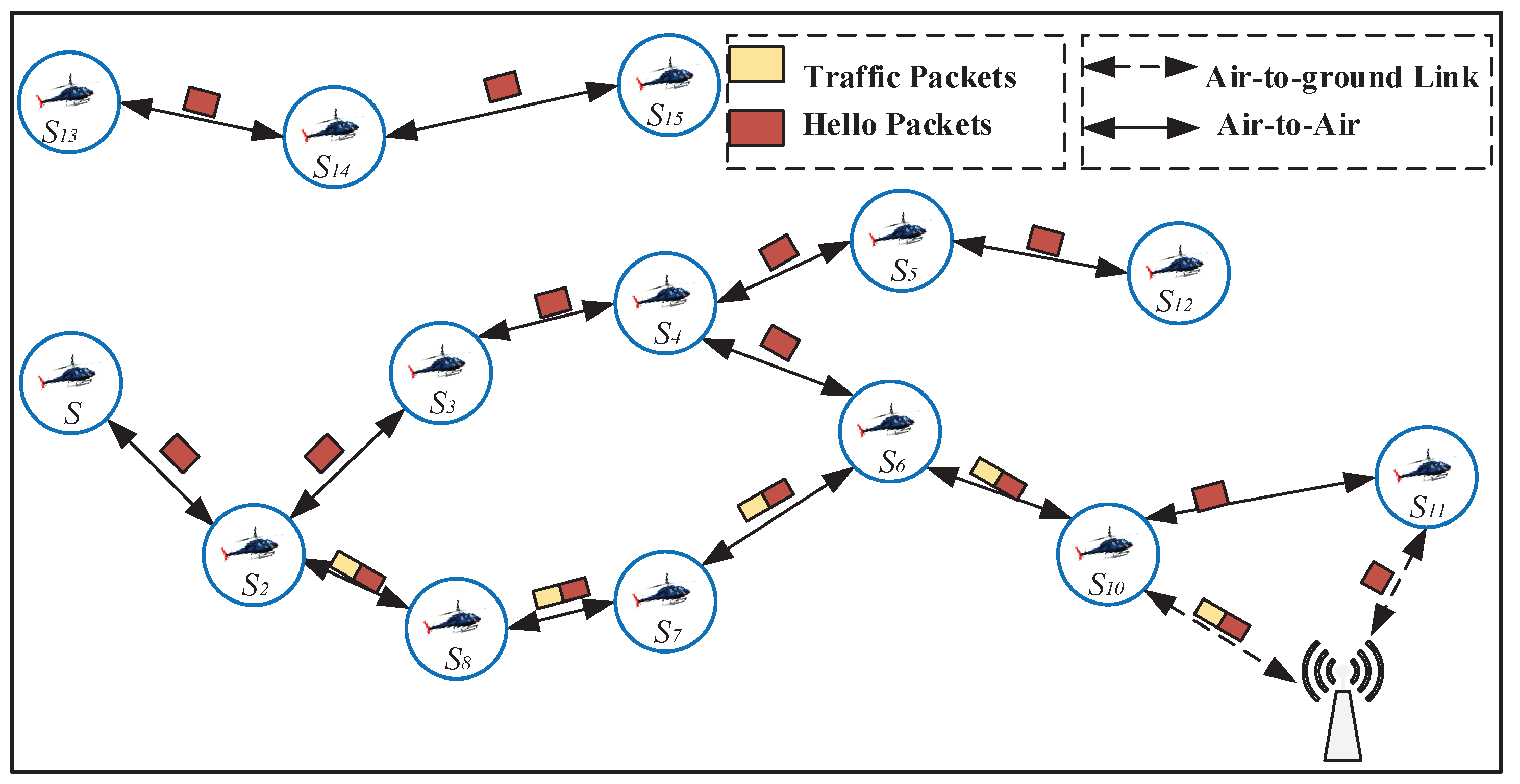
3.2. Neighbors Discovered

In a flying ad hoc network, the high-speed movement of nodes leads to challenges in accurately reflecting the actual position changes of neighbor nodes in the neighbor node list, causing neighbor node information to become outdated. To address this issue, this section proposes an efficient neighbor node discovery algorithm. The core objective of this algorithm is to rapidly eliminate outdated neighbor information and dynamically adjust the sending interval of Hello packets to ensure timely discovery of new messages while reducing the overhead of Hello packet probing.The node sends a Hello packet to its neighboring nodes, which contains its own GPS coordinate information, speed information, and adjacency table. The neighboring nodes also need to respond to their Hello packet once they receive it. Each node maintains a network topology graph in the form of an adjacency table, and uses EKF to predict the neighbor positions of one hop within the interval of Hello packets. As the neighbor discovery process progresses, the adjacency table is continuously updated, and each node in the network will know its reachability to other nodes.

Assuming the distance between two nodes is $d_{ij}\left(t\right)$, the coordinates of node j at time t are $(x_j\left(t\right),y_j\left(t\right),z_j\left(t\right))$, and the coordinates of node i at time t are $(x_i\left(t\right),y_i\left(t\right),z_i\left(t\right))$, then the distance formula between the two nodes at time t is expressed as follows:

$$d_{ij}\left(t\right)=\sqrt{{(x_j\left(t\right)-x_i\left(t\right))}^2+{(y_j\left(t\right)-y_i\left(t\right))}^2+{(z_j\left(t\right)-z_i\left(t\right))}^2}$$

(9)

If $d_{ij}\left(t\right)$ is greater than the transmission range R, it is deemed that the position of neighbor node j of node i at time t is invalid. Node i will then delete the corresponding neighbors and their connections. Sending Hello messages in dynamic time slots greatly reduces the overhead of neighbor discovery compared to sending Hello messages in fixed time slots, and nodes can also perceive neighbor departures in a timely manner.

If the predictable inter-node distance $d_{ij}\left(t\right)$ is less than the transmission range R, in order to ensure the timely capture of new messages, we dynamically adjust the transmission time of Hello packets. Given the limitations of periodic broadcast of Hello packets in responded highly dynamic mobile environments, nodes can estimate the expected duration of the link after obtaining their own and neighbors’ location information. The Hello packet transmission interval is flexibly adjusted based on the minimum link duration. Through this approach, when the relative distance between two nodes is expected to exceed the transmission range, the algorithm can more effectively adapt to rapid changes in network topology, ensuring the continuity and timeliness of communication. The link maintenance time between two nodes is represented as follows:

$$L_{t(i,j)}={\displaystyle \frac{|R-d_{ij}\left(t_2\right)|}{△d_{ij}/(t_2-t_1)}}$$

(10)

$$△d_{ij}=d_{ij\left(t_2\right)}-d_{ij\left(t_1\right)}$$

(11)

where $L_{t(i,j)}$ represents the link duration between node i and node j, $d_{ij}$ represents the displacement difference between node i and node j over two time intervals, $△d_{ij}/(t_2-t_1)$ represents the relative velocity between the two nodes, and $|R-d_{ij}\left(t_2\right)|$ represents the distance at which the communication range will be exited. Each node measures the minimum link duration with all its neighbor nodes. Based on the link duration of neighbor nodes, the Hello packet transmission interval needs to be set as follows:

$$T_h=\underset{j\in neighbor\left(i\right)}{min}{L}_{t(i,j)}$$

(12)

$$Hell{o}_t=\tau \ast T_h,0<\tau <1$$

(13)

where $\tau$ is the time update coefficient. By dynamically adjusting the transfer time of Hello packets, it is possible to promptly detect the arrival of new neighbors, laying the foundation for routing decisions. The practical significance of this mechanism is that nodes can predict the possibility of topology changes and actively send Hello packets when changes occur in order to quickly adapt to changes in the network environment.

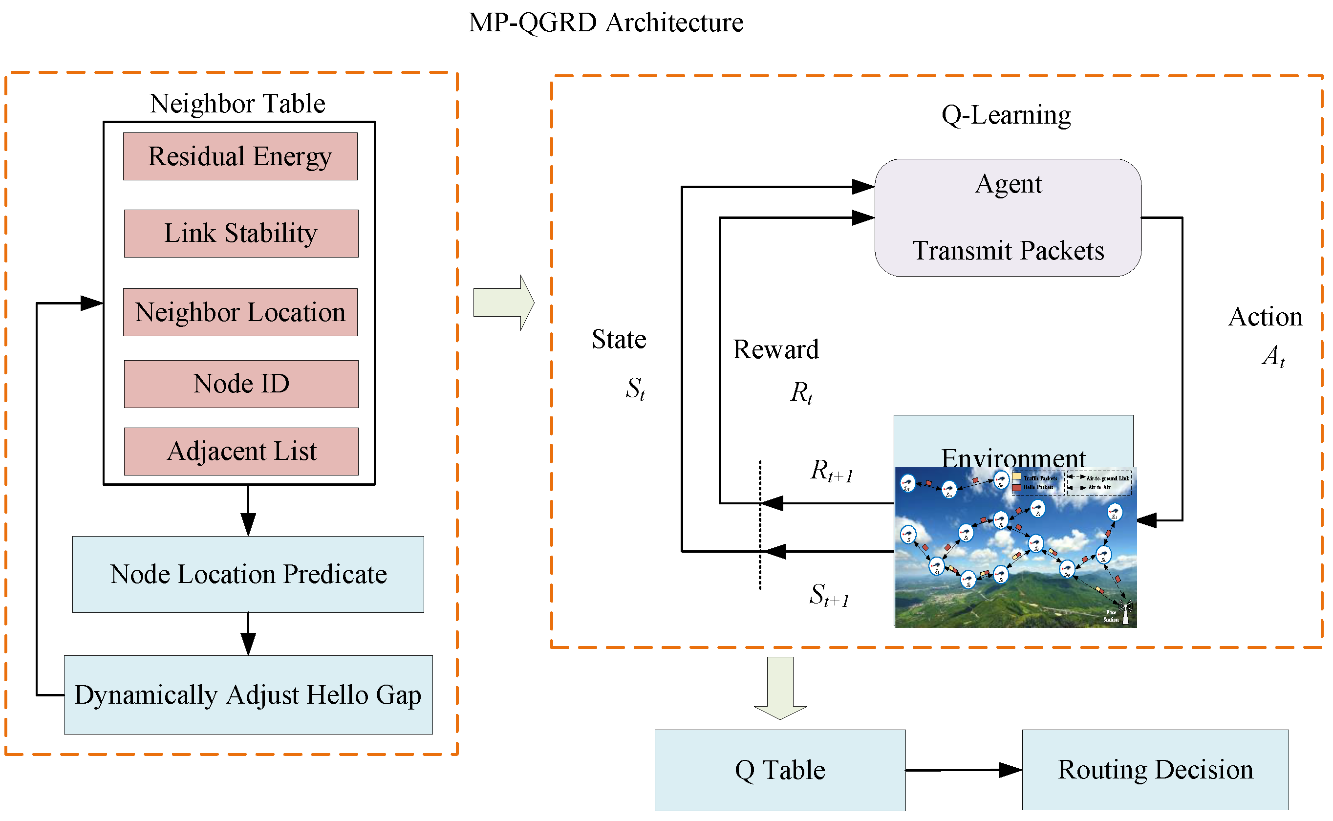
3.3. Routing Decisions

In the process of routing decisions within high dynamic flying ad hoc networks, data packets are sent from the source node, relayed through a series of intermediate nodes, and ultimately reach the destination node. The learning process of the MP-QGRD algorithm focuses on finding an optimal transmission path for these data packets. This algorithm is primarily composed of three key steps: mobility prediction, neighbor discovery, and routing decision. Mobility prediction is responsible for forecasting the dynamic changes of nodes within the network, neighbor discovery is used to update the neighbor information of nodes in real-time, and the routing decision, based on the information from the first two steps and the Q-learning algorithm, selects the optimal forwarding path for the data packets. The overall architecture of the MP-QGRD algorithm is illustrated in Figure 2. Through the close collaboration of these steps, the algorithm ensures that data packets can be forwarded to their destination according to the optimal strategy.

In flying ad hoc networks, Q-learning can be applied to problems such as routing selection and resource allocation. By defining states, actions, and reward functions, the flying ad hoc network can be modeled as a Markov decision process (MDP), and the Q-learning algorithm can be used to learn the optimal routing strategy. Utilizing Q-learning to model the process of data packet forwarding between nodes in a given Markov decision process, agents can select the optimal action based on the current state and update the corresponding Q-values by observing the reward signals. The model is defined as follows:

(1)

Agent: The data packets transmitted by each node in the network represent the agents.

(2)

Environment: The entire flying ad hoc network serves as the learning environment for the agents.

(3)

State space: The set of all nodes’ states.

(4)

Action space: The action space of the agents is the set of neighbor nodes. Selecting a node from the set of neighbors as the next hop for the data packet constitutes an action.

(5)

Reward function: The immediate reward value provided by the entire flight network to the nodes. The reward function is designed based on metrics such as link stability, distance to the destination, and energy consumption, aiming to enable nodes to adapt to the dynamic network environment.

Design of the Reward Function

Calculate the link stability factor. The link stability between nodes is one of the key factors in selecting reliable paths, ensuring stable packet transmission. If node i and node j can communicate with each other, the communication quality factor and link time factor between the two nodes can be represented as follows:

$$L{Q}_{(i,j)}={\displaystyle \frac{P_{(i,j)r}}{P_{(i,j)t}}}$$

(14)

$$L{P}_{(i,j)}={\displaystyle \frac{R-d_{ij}}{R}}$$

(15)

where $P_{(i,j)r}$ and $P_{(i,j)t}$ represent the number of data packets received for node i to node j and the total number of data packets sent by node i, respectively, R represents the communication radius of the node, and $d_{ij}$ represents the communication distance between two nodes. Therefore, the measure of link stability between nodes is expressed as follows:

$$L{S}_{(i,j)}=\lambda L{Q}_{(i,j)}+(1-\lambda )L{P}_{(i,j)}$$

(16)

where $L{S}_{(i,j)}$ represents the link stability, with higher values indicating greater stability between the two nodes.

Calculate the energy factor. To prevent certain nodes from being excessively drained and to ensure that each node can operate sustainably and stably, the remaining energy status of each node must be fully considered. This section specifically introduces the energy factor as a metric for measuring the energy consumption level of nodes. The energy factor not only reflects the current remaining energy status of the node but also provides a reliable basis for energy consumption during route selection. By effectively utilizing the energy factor, it ensures that data can be forwarded to the next hop by selecting nodes with sufficient energy and higher reliability, thereby optimizing the energy utilization efficiency of the network and prolonging the overall lifespan of the network. The energy factor is defined as follows:

$$E_{\left(i\right)N}={\displaystyle \frac{E_{\left(i\right)R}}{E_{\left(i\right)I}}}-k{d_{i,j}}^2$$

(17)

where $E_{\left(i\right)R}$ represents the remaining energy of node i, with higher values indicating greater stability between the two nodes. $E_{\left(i\right)N}$ is the cost function for the remaining energy, and $E_{\left(i\right)I}$ denotes the initial energy of node i. Since all nodes have the same initial energy level, a larger $E_{\left(i\right)N}$ leads to relatively lower energy consumption for the node.

Calculate the distance factor. To accurately assess the distance between neighbor nodes and the target node, this paper introduces the concept of a distance factor. This factor comprehensively considers the relative position of neighbor nodes to the target node and the distance between this node and the target node. The calculation of the distance factor is as follows:

$$D{F}_i(j,d)=\left\{\begin{array}{cc}cos\theta \times e^{\frac{D(i,d)-D(j,d)}{R}}-1,\hfill & d_{ij}<R\hfill \\ 0,\hfill & otherwise\hfill \end{array}\right.$$

(18)

where i, j, and d represent the predicted positions of the current node, neighbor node, and destination node, respectively. R denotes the transmission range of the current node, while $\theta$ represents the angle between the current node, destination node, and neighbor node. $d_{ij}$ represents the Euclidean distance between the predicted positions of the two nodes. The consideration of distance factor ensures that the routing transmission quickly approaches the target node.

By comprehensively considering distance measurement, link stability measurement, and residual energy measurement, a reward function is constructed, which is expressed as follows:

$$r={\lambda }_{1}D{F}_i(j,d)+{\lambda }_{2}L{S}_{(i,j)}+{\lambda }_3{E}_{\left(i\right)N}$$

(19)

where $D{F}_i(j,d)$ represents the distance metric, $L{S}_{(i,j)}$ represents the link stability metric, and $E_{\left(i\right)N}$ represents the residual energy metric of node. A higher value of the reward function r indicates that the action taken is optimal under the current state.

Adaptive learning parameters

In high dynamic flying ad hoc networks, the link status between nodes often changes. Fixed Q-learning parameters cannot adapt to frequent link changes caused by the high-speed movement of nodes. Therefore, it is necessary to adaptively adjust the learning rate and discount factor to accommodate link breaks caused by the high-speed movement of nodes. In this section, the learning rate is adjusted based on link stability, and the discount factor is adaptively adjusted based on node mobility. The formula for calculating the learning rate is as follows:

$$\alpha =\left\{\begin{array}{cc}1-e^{-LS(i,j)},\hfill & \sigma (i,j)\ne 0\hfill \\ 0.3,\hfill & \sigma (i,j)=0\hfill \end{array}\right.$$

(20)

where $LS(i,j)$ is the link stability indicator between nodes i and j, and $\sigma (i,j)$ is the variance of $LS(i,j)$.

Based on the mobility of nodes, the range of dynamic discount factors $\gamma$ is considered in this section. When the expected neighbor node is within the communication range of the node, it will provide a higher discount value. A higher discount factor indicates that the expected Q-value will remain stable. The mobility and availability of neighbor nodes are important factors because considering these factors in routing decisions aims to find suitable nodes for forwarding. The discount factor for any node is defined as follows:

$$\gamma =\sqrt{{\displaystyle \frac{|N_{i(t-1)}\cap N_{i\left(t\right)}|}{|N_{i(t-1)}\cup N_{i\left(t\right)}|}}}$$

(21)

where $\gamma$ represents the discount factor, $N_{i\left(t\right)}$ represents the set of neighbors of the current node i at the current time, and $N_{i(t-1)}$ represents the set of neighbors of the previous node i at the time $t-1$. When the desired neighbor node is within the communication range of the node, it will provide a higher discount value. A higher discount factor indicates that the nodes within the neighbor set are more stable.

After defining the reward function, adaptive learning rate, and discount factor, the update function for the Q-value is as follows:

$$\begin{array}{c}\hfill NewQ(s_t,a_t)\leftarrow Q(s_t,a_t)+\alpha [r+\gamma \times \underset{a}{max}Q(s_{t+1},a_{t+1})-Q(s_t,a_t)]\end{array}$$

(22)

where $\alpha$ is the learning rate, $\gamma$ is the discount factor, $Q(s_t,a_t)$ represents the Q-value of state $s_t$ at time t, and r is the immediate reward value obtained by the agent for taking action $a_t$ in state $s_t$ at time t. After the agent executes action $a_t$, the state of the agent transitions from state $s_t$ to state $s_{t+1}$. ${max}_{a}Q(s_{t+1},a_{t+1})$ represents the expected future Q-value, which is the maximum Q-value when the agent chooses to take action $a_{t+1}$ in the next state $s_{t+1}$.

3.4. Algorithm Design

The main algorithm is shown in Algorithm 1. Nodes obtain real-time location and velocity information through GPS positioning, and integrate this information into the Hello packet. Nodes use the extended Kalman filter algorithm to predict their movement trajectories, and dynamically adjust the sending interval of Hello packets based on the predicted results. In addition, nodes can also predict the moment when a neighboring node exceeds the communication range. Additionally, the algorithm dynamically adjusts the interval for sending Hello packets according to Equation (13), enabling timely discovery of new neighbors and real-time update of the neighbor table.

The algorithm utilizes Q-learning for routing decisions according to the neighbor list is shown in Algorithm 2. Considering the link stability, energy consumption, and distance to the destination, a reward function is constructed based on these three metrics to determine candidate forwarding nodes. Adaptive learning parameters are built based on node stability and mobility, dynamically adjusting the learning rate according to link stability and adjusting the discount factor based on node mobility. Through Equation (22), the Q-value function is updated, and the node with the highest Q-value is selected as the forwarding node, ensuring efficient and reliable data transmission.

Algorithm 1 Neighbor discovery

Input:  Node i receives a Hello packet from neighbor j Output:  Node i update the Neighbor Table, dynamically adjust Hello interval 1: Get Attributes $x_t$, $y_t$, $z_t$, $v_{x,t}$, $v_{y,t}$, $v_{z,t}$ from Hello packet 2: for time_point $t_a$: $(Hell{o}_{t-1}\times 2)$ do 3:     Predict the movement state $X_{t_a}$ of Node i and j according to EKF 4:     Calculate the distance $d_{ij}\left(t_a\right)$ based on Equation (9) 5:     if $d_{ij}\left(t_a\right)$ > R then 6:         Node $j_{t_2}$ = $t_a$ 7:         Calculate the Link maintenance time $L_{t_2(i,j)}$ based on Equation (10) 8:         break for 9:     end if 10: end for 11: Update the Neighbor table 12: Update the Adjacent list 13: Decision the $Hell{o}_t$ based on Equations (12) and (13)

Algorithm 2 Routing decision

Input:  Node i receives a packet from neighbor k Output:  Forwarding packets, adjust algorithm parameters 1: Execute the $Action$ based on Q algorithm 2: choose the max Q value of Node j as next hop 3: Schedule.async(AsynchronousWaitForReward, $S_t$).get() 4: function AsynchronousWaitForReward($S_t$) 5:     Asynchronous Wait for j reply $reward$ 6:     Adaptive learning parameters based on (20) and (21) 7:     Update the Q table based on Equation (22) 8: end function

4. Evaluation

4.1. Experimental Platform

The simulation environment of this paper is Ubuntu 18.04 and Network Simulator 3 (NS-3.29) [37], and it is compared with other routing protocols. The simulation scenarios are distributed within a 1000 m × 1000 m × 1000 m area. The speed of the nodes varies between 10–100 m/s, and the number of nodes is set to 20–100. Each node has the same maximum transmission power of 15 dBm, with a receiving sensitivity of −80 dBm [38]. The corresponding communication radius at maximum transmission power is approximately 250 m. Each node communicates using IEEE 802.11p [39], and all nodes have the same initial energy.

Table 1. Experiment parameters.

Simulation Parameters	Value
Simulation area	1000 × 1000 × 1000 m3
Number of nodes	20–100 pieces
Node speed	10–100 m/s
Physical layer	802.11 p
Max TxPower (transmission power)	15 dBm
MiniRssi (receiving sensitivity)	−80 dBm
Signal propagation loss model	ITU-R 1411 log distance propagation
Packet size	64–1024 Bytes
$\tau$	0.6
Communication radius	about 250 m
Mobile model	3D Gaussian Markov Moving Model
the number of repetitions	20/for each different algorithm
$\gamma$ update interval	100 ms
${\lambda }_1$, ${\lambda }_2$, ${\lambda }_3$	0.4 0.3 0.3
Simulation time	300 s

shows the experimental parameter settings for the simulation.

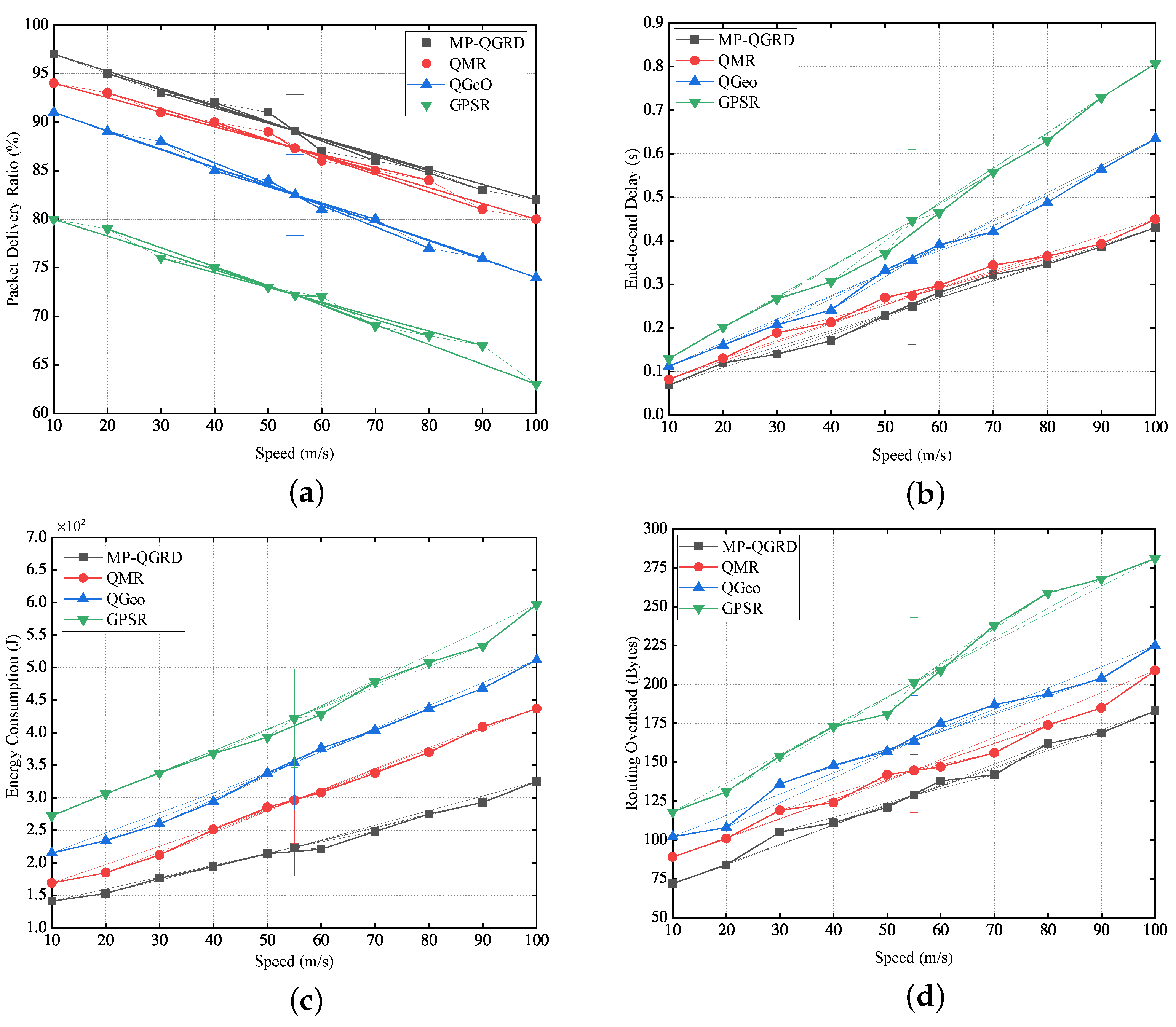
4.2. Comparison of Experimental Results

In this section, the simulation results of the MP-QGRD algorithm will be analyzed and compared with three routing protocols: QMR [35], QGeo [34], and GPSR [13].

QGeo combines Q-learning with geographic routing to evaluate the effectiveness of historical forwarding through Q-values, and prioritizes selecting neighboring nodes with high transmission success rates and stable paths. However, without considering node mobility and link interruption, and the Hello message being broadcasted at fixed intervals, it is difficult to adapt to rapid topology changes. QMR evaluates path quality (latency, link stability) based on Q-values and dynamically selects paths with higher Q-values to forward data. QMR takes into account energy consumption factors, but still uses a fixed cycle to send Hello messages, without considering link changes in high dynamic environments, resulting in delayed path selection. GPSR is a classic geographic location routing protocol that uses greedy and perimeter forwarding to prioritize the nearest neighbor node to the target, achieving fast path selection. However, neglecting link quality and stability can easily lead to the impact of link breakage, resulting in an increase in data loss rate.

MP-QGRD combines motion prediction and Q-learning, using an extended Kalman filter (EKF) to predict the positions of adjacent nodes, evaluate link stability and duration, and adopt an adaptive Hello mechanism to detect the positions of neighboring nodes. At the same time, the algorithm introduces a Q-learning mechanism in routing decision-making, dynamically selecting the best performing node for data forwarding based on the link stability and transmission performance of adjacent nodes.

We conducted multiple repeated experiments on four algorithms, comparing them in terms of packet delivery ratio, end-to-end delay, communication energy consumption, routing overhead. Among them, communication energy consumption refers to the average communication energy consumption of UAV nodes during the simulation process, measured in joules (J). The calculation method is to multiply the single communication signal transmission power by the single communication transmission duration and, finally, perform unit conversion.

Figure 3 shows the evaluation metrics corresponding to a fixed number of 50 UAV nodes. Figure 3a illustrates how the packet delivery ratio (PDR) varies with node speed. As the node speed increases, the high speed of drones will lead to more unstable communication links, and the performance of all four routing protocols declines. Among them, the GPSR routing protocol exhibits the poorest routing performance. QMR, compared to QGeo, considers link stability, resulting in better packet delivery rates. Due to the faster speed and the worse link status, this protocol accurately predicts the location in the next moment using the extended Kalman filter model to deliver data to nodes with good link quality. Therefore, MP-QGRD demonstrates the best PDR performance. MP-QGRD reduces the average link interruption rate by 10% through mobile prediction and the adaptive Hello packet adjustment mechanism.

Figure 3b compares the delay performance of the four protocols. As node speed increases, GPSR exhibits more routing errors compared to QGeo, leading to increasing delays. In contrast, QMR and MP-QGRD demonstrate more adaptability. QMR selects nodes with lower delays for routing decisions, but rapid changes in neighbor nodes cause routing changes and increased delays. MP-QGRD accurately predicts node positions and selects nodes closer to the destination as relays. Therefore, MP-QGRD outperforms QMR in delay performance.

Figure 3c shows that as nodes move faster, their communication energy consumption continues to increase. GPSR and QGeo routing protocols do not consider energy consumption, resulting in relatively high energy consumption. QMR and MP-QGRD consider energy consumption in their reward functions, but MP-QGRD also considers link retention time and sets an energy threshold, selecting nodes with energy above the threshold for data transmission. Therefore, the energy consumption of the MP-QGRD routing protocol is lower than that of other routing protocols.

Figure 3d demonstrates that as node speed increases, the routing overhead of the four protocols continues to rise. GPSR is a stateless protocol, where the rapid movement of nodes leads to frequent changes in the topology structure and a high number of route retransmissions, resulting in gradually increasing routing overhead. However, QGeo shows lower overhead compared to GPSR by Q-learning technology. Although QMR introduces a neighbor discovery mechanism, it does not dynamically adjust the sending interval of Hello packets to promptly discover dynamic neighbor changes, leading to increased routing overhead. Dynamically adjusting the sending interval of Hello packets during neighbor discovery reduces routing overhead. Therefore, the routing overhead of MP-QGRD is the lowest. The strategy of sending Hello packets at fixed time intervals will result in an average increase of about 15–20% in communication overhead.

To further demonstrate the performance of our algorithm, we presented the changes in metrics corresponding to different numbers of drone nodes at an average movement speed of 70 m/s.

Figure 4a illustrates how the packet delivery ratio of the four routing protocols increases as the number of nodes increases. Among them, MP-QGRD outperforms the others significantly. MP-QGRD enhances relay node availability through mobility prediction and selects the most stable link for forwarding. As the number of nodes increases, network connectivity improves, resulting in higher PDR. GPSR performs the poorest due to its reliance solely on node positions rather than global information. QGeo, by employing Q-learning to select the optimal path, outperforms GPSR. QMR, by evaluating neighbor relationships to determine the best node for forwarding, performs better than QGeo.

Figure 4b demonstrates the impact of node count changes on end-to-end delay. MP-QGRD exhibits the lowest latency in low-density networks by reducing routing construction time through accurate position prediction. Although delays increase with more nodes, MP-QGRD remains significantly lower than other protocols. MP-QGRD reduces delay by selecting reliable links using Q-learning. GPSR experiences the longest delay due to its perimeter forwarding mechanism. QMR, considering delay metrics, outperforms QGeo. MP-QGRD predicts node positions and selects the nearest node to the destination for forwarding, achieving low latency.

Figure 4c shows the communication energy consumption of the four routing protocols under different node counts. MP-QGRD and QMR consume less energy than QGeo and GPSR. The former considers node energy consumption when designing the reward function, so it selects the next hop node with lower energy consumption for forwarding. Additionally, MP-QGRD considers remaining energy of a node, allowing only nodes with an energy level exceeding the threshold to participate in communication. Therefore, MP-QGRD has the lowest energy consumption level.

Figure 4d demonstrates that as the number of nodes increases, the routing overheads of MP-QGRD, QMR, QGeo, and GPSR protocols all steadily increase. With the increase in node density, the GPSR routing protocol experiences an increase in control message quantity. The rapid movement of nodes also leads to frequent changes in the network topology, resulting in more routing retransmissions and thus increased routing overhead. QGeo and QMR, by introducing Q-learning technology, can perceive changes in the network environment and reduce some routing overhead during routing decisions. MP-QGRD, through mobility prediction, can avoid invalid node connections before link disconnection, reducing routing overhead. Therefore, MP-QGRD exhibits the lowest routing overhead.

Based on the above analysis, MP-QGRD improves the stability of wireless links through location prediction. Using dynamic time slots to send Hello messages effectively reduces congestion on wireless links, thereby improving the success rate of data transmission. Meanwhile, by integrating reinforcement learning methods and considering multiple factors, the energy consumption of network communication has been further optimized.

5. Discussion

The extended Kalman filter model is used to predict node positions, with a computational complexity of $O\left(n\right)$, where n is the number of nodes. The neighbor discovery process requires real-time calculation of neighbor distances and updating of the adjacency table, with a time complexity of $O\left(n^2\right)$. Although the time complexity of neighbor discovery is relatively high, due to the dynamic adjustment and intermittency of Hello packet transmission, the actual calculation frequency is low, effectively reducing the computational burden. Therefore, although there may be certain computational challenges in large-scale networks, the resource consumption in practical applications is controllable.

Although MP-QGRD performs well under existing experimental conditions, we also recognize that this approach still has certain limitations. For example, in larger-scale FANET environments, the dynamic Hello packet adjustment strategy and the computational cost of Q-learning models may need further optimization. Future research will focus on exploring the adaptability of MP-QGRD in different network scales and various mobile modes to ensure its superior performance in a wider range of application scenarios.

6. Conclusions

In this article, we propose a geographic routing decision method based on extended Kalman filtering and Q-learning, aimed at addressing the instability of links caused by frequent changes in node positions and energy limitations in flying ad hoc networks. By accurately predicting the movement trajectory of nodes, we have designed a mechanism for dynamically adjusting the Hello packet transmission time slot, thereby optimizing the neighbor discovery process and effectively reducing communication energy consumption. At the same time, combined with the Q-learning algorithm, we propose an intelligent routing decision strategy that comprehensively considers link stability, communication distance, and energy consumption. The simulation results have verified that the MP-QGRD method exhibits significant advantages over existing routing schemes in terms of data transmission success rate, latency, and energy consumption control. With the expansion of network scale, the computational complexity and real-time response capability of algorithms remain controllable.

References

1. Pasandideh, F.; Costa, J.P.J.; Kunst, R.; Hardjawana, W.; Freitas, E.P. A systematic literature review of flying ad hoc networks: State-of-the-art, challenges, and perspectives. J. Field Robot. 2023, 40, 955–979. [Google Scholar]
2. Lansky, J.; Rahmani, A.M.; Malik, M.H.; Yousefpoor, E.; Yousefpoor, M.S.; Khan, M.U.; Hosseinzadeh, M. An energy-aware routing method using firefly algorithm for flying ad hoc networks. Sci. Rep. 2023, 13, 1323. [Google Scholar]
3. Srivastava, A.; Prakash, J. Future FANET with application and enabling techniques: Anatomization and sustainability issues. Comput. Sci. Rev. 2021, 39, 100359. [Google Scholar]
4. Ceviz, O.; Sen, S.; Sadioglu, P. A Survey of Security in UAVs and FANETs: Issues, Threats, Analysis of Attacks, and Solutions. IEEE Commun. Surv. Tutorials 2024. [Google Scholar] [CrossRef]
5. Gaydamaka, A.; Samuylov, A.; Moltchanov, D.; Ashraf, M.; Tan, B.; Koucheryavy, Y. Dynamic topology organization and maintenance algorithms for autonomous UAV swarms. IEEE Trans. Mob. Comput. 2023, 23, 4423–4439. [Google Scholar] [CrossRef]
6. Wang, C.M.; Yang, S.; Dong, W.Y.; Zhao, W.; Lin, W. A Distributed Hybrid Proactive-Reactive Ant Colony Routing Protocol for Highly Dynamic FANETs with Link Quality Prediction. IEEE Trans. Veh. Technol. 2024, 74, 1817–1822. [Google Scholar]
7. Tang, F.; Hofner, H.; Kato, N.; Kaneko, K.; Yamashita, Y.; Hangai, M. A deep reinforcement learning-based dynamic traffic offloading in space-air-ground integrated networks (SAGIN). IEEE J. Sel. Areas Commun. 2021, 40, 276–289. [Google Scholar]
8. Lin, N.; Huang, J.; Hawbani, A.; Zhao, L.; Tang, H.; Guan, Y.; Sun, Y. Joint routing and computation offloading based deep reinforcement learning for Flying Ad hoc Networks. Comput. Netw. 2024, 249, 110514. [Google Scholar]
9. Zhang, Z.; Li, X.; Wang, Y.; Miao, Y.; Liu, X.; Weng, J.; Deng, R.H. TAGKA: Threshold authenticated group key agreement protocol against member disconnect for UANET. IEEE Trans. Veh. Technol. 2023, 72, 14987–15001. [Google Scholar]
10. Oubbati, O.S.; Mozaffari, M.; Chaib, N. ECaD: Energy-efficient routing in flying ad hoc networks. Int. J. Commun. Syst. 2019, 32, 41–56. [Google Scholar]
11. Pramitarini, Y.; Perdana, R.H.Y.; Shim, K. Federated Blockchain-Based Clustering Protocol for Enhanced Security and Connectivity in FANETs With CF-mMIMO. IEEE Internet Things J. 2025. [Google Scholar] [CrossRef]
12. Hong, J.; Zhang, D. TARCS: A topology change aware-based routing protocol choosing scheme of FANETs. Electronics 2019, 8, 274. [Google Scholar] [CrossRef]
13. Alsaqour, R.; Abdelhaq, M.; Saeed, R.; Uddin, M.; Alsukour, O.; Al-Hubaishi, M.; Alahdal, T. Dynamic packet beaconing for GPSR mobile ad hoc position-based routing protocol using fuzzy logic. J. Netw. Comput. Appl. 2015, 47, 32–46. [Google Scholar] [CrossRef]
14. Zhu, R.; Jiang, Q.; Huang, X.; Li, D.; Yang, Q. A reinforcement-learning-based opportunistic routing protocol for energy-efficient and Void-Avoided UASNs. IEEE Sens. J. 2022, 22, 13589–13601. [Google Scholar]
15. Swain, S.; Khilar, P.M.; Senapati, B.R. A reinforcement learning-based cluster routing scheme with dynamic path planning for mutli-uav network. Veh. Commun. 2023, 41, 100605. [Google Scholar] [CrossRef]
16. Kayhani, N.; Zhao, W.; McCabe, B.; Schoellig, A.P. Tag-based visual-inertial localization of unmanned aerial vehicles in indoor construction environments using an on-manifold extended Kalman filter. Autom. Constr. 2022, 135, 104112. [Google Scholar] [CrossRef]
17. Xiang, X.; Wang, X.; Zhou, Z. Self-adaptive on-demand geographic routing for mobile ad hoc networks. IEEE Trans. Mob. Comput. 2011, 11, 1572–1586. [Google Scholar] [CrossRef]
18. Saini, T.K.; Sharma, S.C. Recent advancements, review analysis, and extensions of the AODV with the illustration of the applied concept. Ad Hoc Netw. 2020, 103, 102148. [Google Scholar] [CrossRef]
19. Bai, R.; Singhal, M. DOA: DSR over AODV routing for mobile ad hoc networks. IEEE Trans. Mob. Comput. 2006, 5, 1403–1416. [Google Scholar]
20. Wang, H.; Li, Y.; Zhang, Y.; Huang, T.; Jiang, Y. Arithmetic optimization AOMDV routing protocol for FANETs. Sensors 2023, 23, 7550. [Google Scholar] [CrossRef]
21. Sarkar, D.; Choudhury, S.; Majumder, A. Enhanced-Ant-AODV for optimal route selection in mobile ad-hoc network. J. King Saud-Univ.-Comput. Inf. Sci. 2021, 33, 1186–1201. [Google Scholar]
22. Joon, R.; Tomar, P. Energy aware Q-learning AODV (EAQ-AODV) routing for cognitive radio sensor networks. J. King Saud-Univ.-Comput. Inf. Sci. 2022, 34, 6989–7000. [Google Scholar] [CrossRef]
23. Mohamed, R.E.; Ghanem, W.R.; Khalil, A.T.; Elhoseny, M.; Sajjad, M.; Mohamed, M.A. Energy efficient collaborative proactive routing protocol for wireless sensor network. Comput. Netw. 2018, 142, 154–167. [Google Scholar]
24. Islam, M.A.; Atat, R.; Ismail, M. Software-Defined Networking Based Resilient Proactive Routing in Smart Grids Using Graph Neural Networks and Deep Q-Networks. IEEE Access 2024, 12, 111169–111186. [Google Scholar]
25. Gangopadhyay, S.; Jain, V.K. A position-based modified OLSR routing protocol for flying ad hoc networks. IEEE Trans. Veh. Technol. 2023, 72, 12087–12098. [Google Scholar]
26. Qiu, X.; Yang, Y.; Xu, L.; Yin, J.; Liao, Z. Maintaining links in the highly dynamic FANET using deep reinforcement learning. IEEE Trans. Veh. Technol. 2022, 72, 2804–2818. [Google Scholar]
27. Asaamoning, G.; Mendes, P.; Magaia, N. A dynamic clustering mechanism with load-balancing for flying ad hoc networks. IEEE Access 2021, 9, 158574–158586. [Google Scholar]
28. Rahmani, A.M.; Ali, S.; Yousefpoor, E.; Yousefpoor, M.S.; Javaheri, D.; Lalbakhsh, P.; Ahmed, O.H.; Hosseinzadeh, M. OLSR+: A new routing method based on fuzzy logic in flying ad-hoc networks (FANETs). Veh. Commun. 2022, 36, 100489. [Google Scholar]
29. Karp, B.; Kung, H.T. GPSR: Greedy perimeter stateless routing for wireless networks. In Proceedings of the 6th Annual International Conference on Mobile Computing and Networking, Boston, MA, USA, 6–11 August 2000; pp. 243–254. [Google Scholar]
30. Zheng, B.; Zhuo, K.; Zhang, H.; Wu, H. A novel airborne greedy geographic routing protocol for flying ad hoc networks. Wirel. Netw. 2022, 30, 4413–4427. [Google Scholar]
31. Arafat, M.Y.; Moh, S. A Q-learning-based topology-aware routing protocol for flying ad hoc networks. IEEE Internet Things J. 2021, 9, 1985–2000. [Google Scholar]
32. Qiu, X.; Xie, Y.; Wang, Y.; Ye, L.; Yang, Y. QLGR: A Q-learning-based Geographic FANET Routing Algorithm Based on Multiagent Reinforcement Learning. KSII Trans. Internet Inf. Syst. 2021, 15, 4244–4274. [Google Scholar]
33. Cui, Y.; Zhang, Q.; Feng, Z.; Wei, Z.; Shi, C.; Yang, H. Topology-aware resilient routing protocol for FANETs: An adaptive Q-learning approach. IEEE Internet Things J. 2022, 9, 18632–18649. [Google Scholar] [CrossRef]
34. Jung, W.S.; Yim, J.; Ko, Y.B. QGeo: Q-learning-based geographic ad hoc routing protocol for unmanned robotic networks. IEEE Commun. Lett. 2017, 21, 2258–2261. [Google Scholar]
35. Liu, J.; Wang, Q.; He, C.; Jaffrès-Runser, K.; Xu, Y.; Li, Z.; Xu, Y. QMR: Q-learning based multi-objective optimization routing protocol for flying ad hoc networks. Comput. Commun. 2020, 150, 304–316. [Google Scholar]
36. Hosseinzadeh, M.; Tanveer, J.; Ionescu-Feleaga, L.; Ionescu, B.S.; Yousefpoor, M.S.; Yousefpoor, E.; Ahmed, O.H.; Rahmani, A.M.; Mehmood, A. A greedy perimeter stateless routing method based on a position prediction mechanism for flying ad hoc networks. J. King Saud-Univ.-Comput. Inf. Sci. 2023, 35, 101712. [Google Scholar] [CrossRef]
37. Carneiro, G.; Fontes, H.; Ricardo, M. Fast prototyping of network protocols through ns-3 simulation model reuse. Simul. Model. Pract. Theory 2011, 19, 2063–2075. [Google Scholar] [CrossRef]
38. Chen, G.; Dong, W.; Zhao, Z.; Gu, T. Accurate corruption estimation in ZigBee under cross-technology interference. IEEE Trans. Mob. Comput. 2018, 18, 2243–2256. [Google Scholar]
39. Dinh, T.D.; Le, D.T.; Tran, T.T.T.; Nguyen, T.A. Flying Ad-Hoc Network for Emergency Based on IEEE 802.11p Multichannel MAC Protocol. In Proceedings of the International Conference on Distributed Computer and Communication Networks, Cham, Switzerland, 14–18 October 2019; Springer International Publishing: Cham, Switzerland, 2019; pp. 479–494. [Google Scholar]
Figure 1. The system model diagram.
Electronics 14 01456 g001
Figure 2. The overall architecture of the MP-QGRD.
Electronics 14 01456 g002
Figure 3. Simulation results of node velocity variation: (a) packet delivery ratio; (b) end-to-end delay; (c) energy consumption in communication; (d) routing overhead.
Electronics 14 01456 g003
Figure 4. Simulation results of changes in the number of nodes: (a) packet delivery ratio; (b) end-to-end delay; (c) energy consumption in communication; (d) routing overhead.
Electronics 14 01456 g004