
A Heuristic Mutation Particle Swarm Optimization Algorithm for Budgeted Influence Maximization with Emotional Competition


Abstract
1. Introduction
- We define the budgeted influence maximization problem with emotional competition mathematically based on a dynamic emotional propagation model over time.
- We design a local structure-sensitive heuristic function to evaluate the potential benefits of individuals, and select ones that promote the spread of positive emotions and inhibit negative emotions.
- We propose a mutation particle swarm optimization method to solve the problem. Experimental results on two real-world networks demonstrate the superiority of our proposed model compared to baseline methods.
2. Related Work
2.1. Influence Maximization
2.2. Emotional Propagation
3. Problem Definition
3.1. Emotional Propagation Model
3.2. Budgeted Influence Maximization
4. Methodology
4.1. Vanilla Greedy Algorithm
| Algorithm 1 The vanilla greedy algorithm |
| Input: G: The social graph. : The initial positive and negative node set. : The size of sub-graph set . K: The budget. Output: S: The seed set.
|
4.2. Heuristic Mutation Particle Swarm Optimization
| Algorithm 2 The HMPSO algorithm |
| Input: N: The number of nodes. E: The adjacency matrix. : The initial positive and negative node set. K: The budget. : The number of particle numbers : The number of iterations. Output: S: The seed set.
|
- Initialization. Lines 3–10 initialize all particles. Half of them are selected based on the highest degree-to-cost ratio, and the other half are selected randomly. Lines 11–13 obtain the initial and of the particle swarm.
- Optimization. Lines 14–23 try to seek a better solution during the iteration cycle. Lines 16–17 update the position vector and velocity vector of the particle to obtain a potentially superior seed. Lines 18–22 determine and record the effectiveness of the current particle swarm.
5. Experiments
5.1. Datasets
5.2. Evaluation Metric
5.3. Experimental Settings
5.4. Baselines
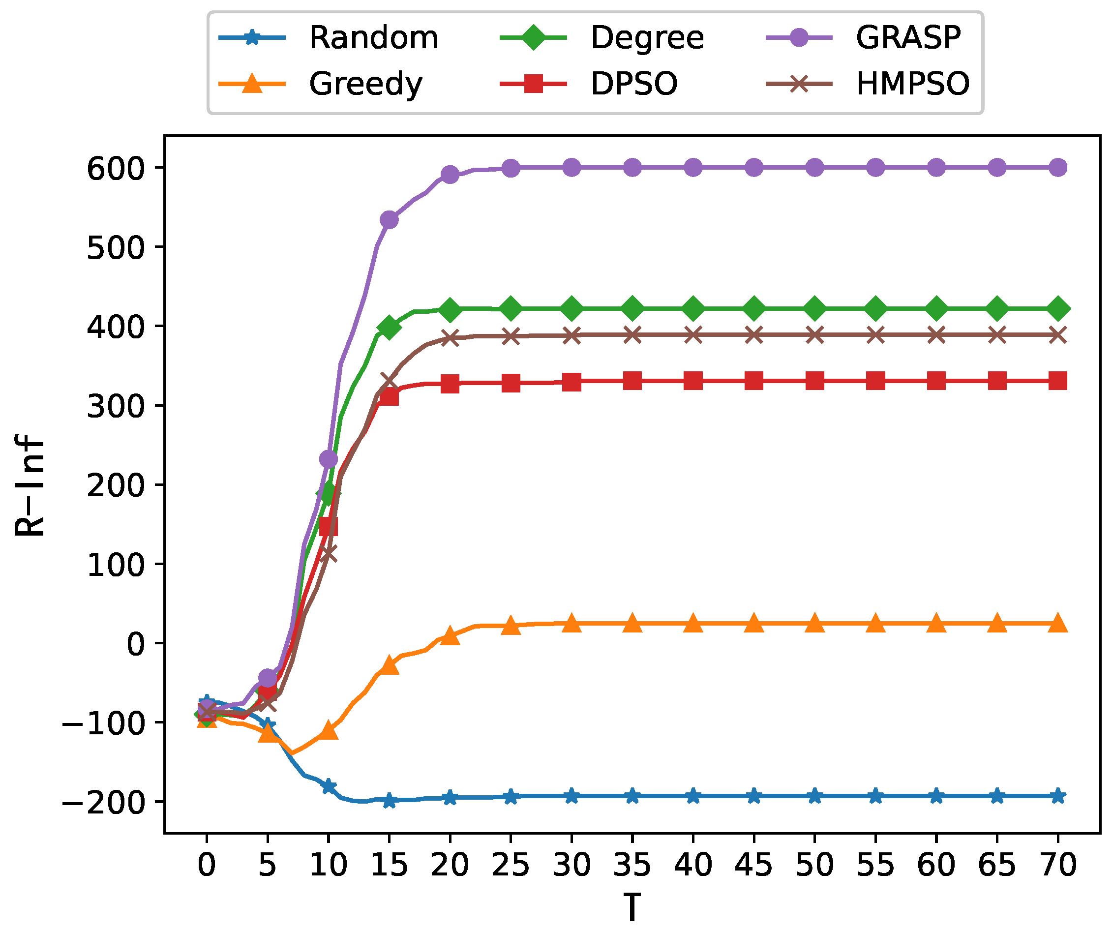
- Classical algorithms: Random is the simplest method. It selects seeds randomly from all nodes; Greedy has been introduced in Section 4.1, i.e., the vanilla greedy algorithm. It selects the seed that brings the highest incremental influence per unit cost within the budget. Degree is an intuitive measurement for choosing the seed. It selects several nodes with the highest degree without exceeding the given budget K as the seed set.
- DPSO [46] is a discrete particle swarm optimization algorithm. It constructs a local influence evaluation function to incorporate the PSO algorithm into the influence maximization problem. The key distinction between the DPSO algorithm and ours is that the DPSO algorithm is designed for the IM problem and does not take into account the budget or emotions.
- GRASP [14] means the greedy randomized adaptive search procedure methodology, which is a multi-start meta-heuristic algorithm. The randomly constructed initial solutions, along with an enhanced local search method, enable the algorithm to mitigate the impact of local optima. It is one of the most effective methods for the BIM problem.
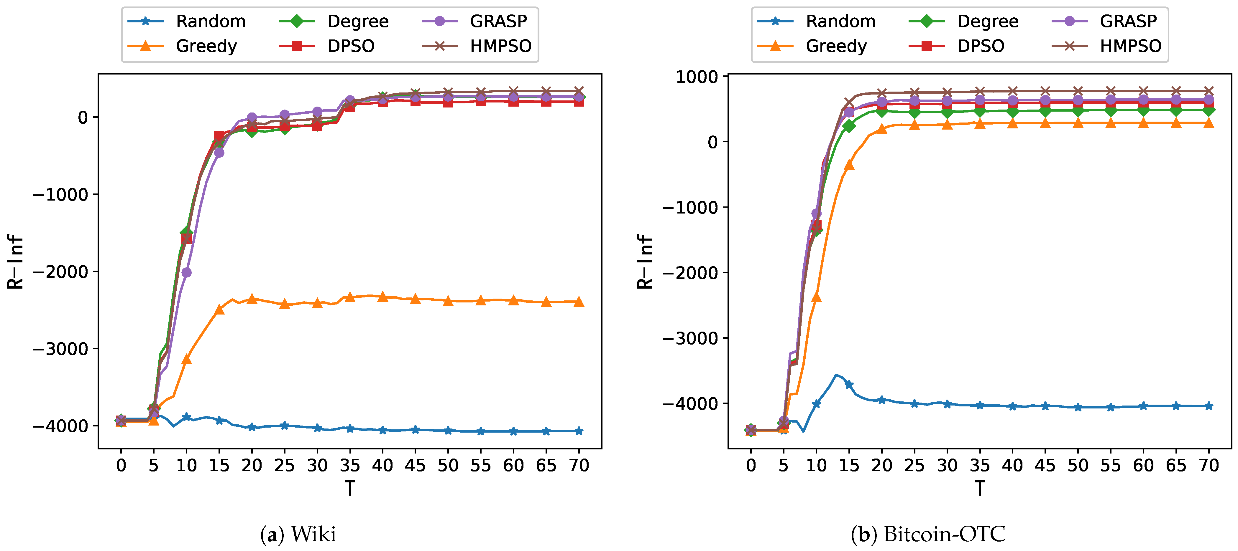
5.5. Comparison Experiments
5.6. Analysis of the Budget
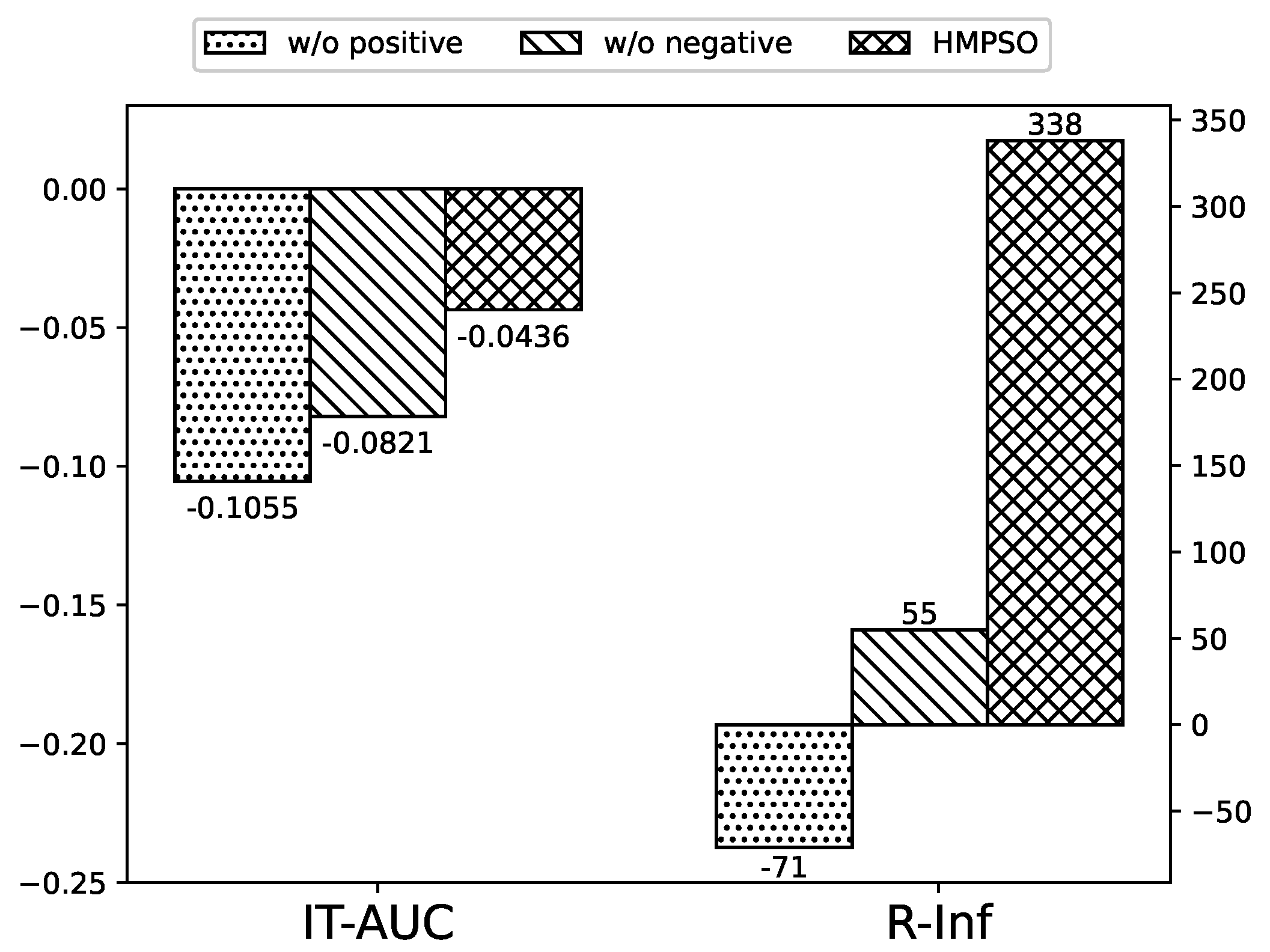
5.7. Ablation Study
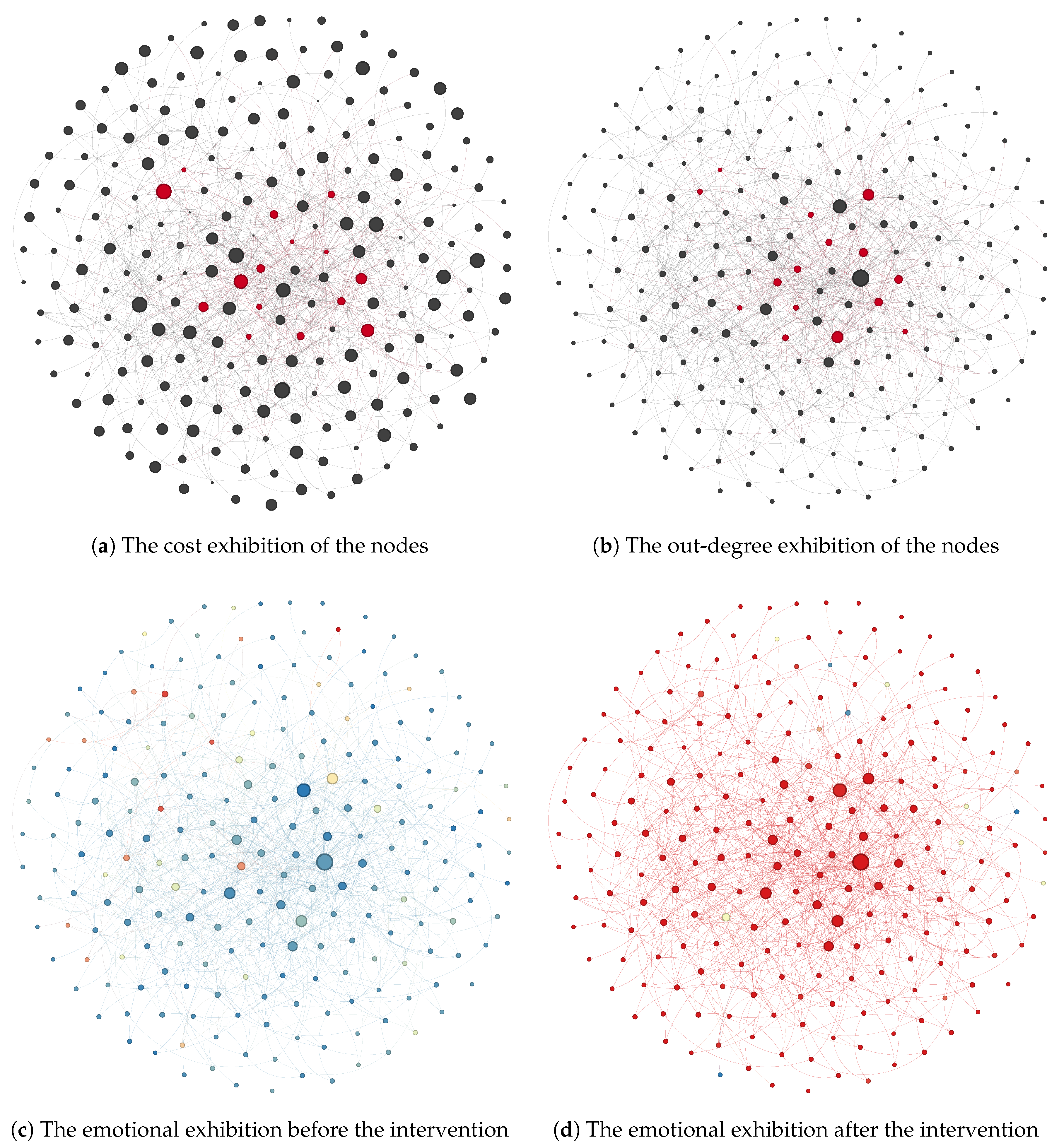
5.8. Case Study
6. Discussion
6.1. Theoretical Implication
6.2. Practical Implication
7. Conclusions
Author Contributions
Funding
Institutional Review Board Statement
Informed Consent Statement
Data Availability Statement
Conflicts of Interest
References
- Kempe, D.; Kleinberg, J.; Tardos, E. Maximizing the spread of influence through a social network. In Proceedings of the Ninth ACM SIGKDD International Conference on Knowledge Discovery and Data Mining, New York, NY, USA, 24–27 August 2003; KDD’03. pp. 137–146. [Google Scholar] [CrossRef]
- Xiong, X.; Li, Y.; Qiao, S.; Han, N.; Wu, Y.; Peng, J.; Li, B. An emotional contagion model for heterogeneous social media with multiple behaviors. Phys. Stat. Mech. Appl. 2018, 490, 185–202. [Google Scholar] [CrossRef]
- Yu, X.; Duan, Y.; Cai, Z.; Luo, W. An adaptive learning grey wolf optimizer for coverage optimization in WSNs. Expert Syst. Appl. 2024, 238, 121917. [Google Scholar] [CrossRef]
- Jusup, M.; Holme, P.; Kanazawa, K.; Takayasu, M.; Romić, I.; Wang, Z.; Geček, S.; Lipić, T.; Podobnik, B.; Wang, L.; et al. Social physics. Phys. Rep. 2022, 948, 1–148. [Google Scholar] [CrossRef]
- Tu, S.; Neumann, S. A Viral Marketing-Based Model For Opinion Dynamics in Online Social Networks. In Proceedings of the ACM Web Conference 2022, New York, NY, USA, 25–29 April 2022; WWW ’22. pp. 1570–1578. [Google Scholar] [CrossRef]
- Huang, L.; Ma, Y.; Liu, Y.; Danny Du, B.; Wang, S.; Li, D. Position-Enhanced and Time-aware Graph Convolutional Network for Sequential Recommendations. ACM Trans. Inf. Syst. 2023, 41, 1–32. [Google Scholar] [CrossRef]
- Li, Y.; Ma, S.; Zhang, Y.; Huang, R.; Kinshuk. An improved mix framework for opinion leader identification in online learning communities. Knowl.-Based Syst. 2013, 43, 43–51. [Google Scholar] [CrossRef]
- Nguyen, H.; Zheng, R. On Budgeted Influence Maximization in Social Networks. IEEE J. Sel. Areas Commun. 2013, 31, 1084–1094. [Google Scholar] [CrossRef]
- Bharathi, S.; Kempe, D.; Salek, M. Competitive Influence Maximization in Social Networks. In Proceedings of the 3rd International Conference on Internet and Network Economics, WINE’07, San Diego, CA, USA, 12–14 December 2007; Deng, X., Graham, F.C., Eds.; Springer: Berlin/Heidelberg, Germany, 2007; pp. 306–311. [Google Scholar]
- Hernandez-Suarez, A.; Sanchez-Perez, G.; Toscano-Medina, K.; Martinez-Hernandez, V.; Perez-Meana, H.; Olivares-Mercado, J.; Sanchez, V. Social Sentiment Sensor in Twitter for Predicting Cyber-Attacks Using l1 Regularization. Sensors 2018, 18, 1380. [Google Scholar] [CrossRef]
- Granovetter, M. Threshold models of collective behavior. Am. J. Sociol. 1978, 83, 1420–1443. [Google Scholar] [CrossRef]
- Goldenberg, J.; Libai, B.; Muller, E. Talk of the network: A complex systems look at the underlying process of word-of-mouth. Mark. Lett. 2001, 12, 211–223. [Google Scholar] [CrossRef]
- Shen, H.; Wang, D.; Song, C.; Barabási, A.L. Modeling and predicting popularity dynamics via reinforced Poisson processes. In Proceedings of the Twenty-Eighth AAAI Conference on Artificial Intelligence, Québec City, QC, Canada, 17–31 July 2014; AAAI Press: Washington, DC, USA, 2014. AAAI’14. pp. 291–297. [Google Scholar]
- Lozano-Osorio, I.; Sánchez-Oro, J.; Duarte, A. An efficient and effective GRASP algorithm for the Budget Influence Maximization Problem. J. Ambient Intell. Humaniz. Comput. 2024, 15, 2023–2034. [Google Scholar] [CrossRef]
- Wu, F.; Huberman, B.A. Novelty and collective attention. Proc. Natl. Acad. Sci. USA 2007, 104, 17599–17601. [Google Scholar] [CrossRef] [PubMed]
- Domingos, P.; Richardson, M. Mining the network value of customers. In Proceedings of the Seventh ACM SIGKDD International Conference on Knowledge Discovery and Data Mining, San Francisco, CA, USA, 26–29 August 2001; KDD ’01. pp. 57–66. [Google Scholar] [CrossRef]
- Chen, W.; Lu, W.; Zhang, N. Time-critical influence maximization in social networks with time-delayed diffusion process. In Proceedings of the Twenty-Sixth AAAI Conference on Artificial Intelligence, Toronto, ON, Canada, 22–26 July 2012; AAAI Press: Washington, DC, USA, 2012. AAAI’12. pp. 592–598. [Google Scholar]
- Li, H.; Pan, L.; Wu, P. Dominated competitive influence maximization with time-critical and time-delayed diffusion in social networks. J. Comput. Sci. 2018, 28, 318–327. [Google Scholar] [CrossRef]
- Cao, J.; Min, H.; Wang, H.; Ma, Z.; Liu, b. Self-Interest Influence Maximization Algorithm Based on Subject Preference in Competitive Environment. Chin. J. Comput. 2019, 42, 1495–1510. [Google Scholar]
- Liang, D.; Duan, W. Large-scale three-way group consensus decision considering individual competition behavior in social networks. Inf. Sci. 2023, 641, 119077. [Google Scholar] [CrossRef]
- He, Q.; Zhang, L.; Fang, H.; Wang, X.; Ma, L.; Yu, K.; Zhang, J. Multistage Competitive Opinion Maximization With Q-Learning-Based Method in Social Networks. IEEE Trans. Neural Netw. Learn. Syst. 2024, 1–11. [Google Scholar] [CrossRef]
- Shi, Q.; Wang, C.; Chen, J.; Feng, Y.; Chen, C. Post and repost: A holistic view of budgeted influence maximization. Neurocomputing 2019, 338, 92–100. [Google Scholar] [CrossRef]
- Banerjee, S.; Jenamani, M.; Pratihar, D.K. ComBIM: A community-based solution approach for the Budgeted Influence Maximization Problem. Expert Syst. Appl. 2019, 125, 1–13. [Google Scholar] [CrossRef]
- Clifford, P.; Sudbury, A. A model for spatial conflict. Biometrika 1973, 60, 581–588. [Google Scholar] [CrossRef]
- Wang, Q.; Lin, Z.; Jin, Y.; Cheng, S.; Yang, T. ESIS: Emotion-based spreader-ignorant-stifler model for information diffusion. Knowl. Based Syst. 2015, 81, 46–55. [Google Scholar] [CrossRef]
- Deffuant, G.; Neau, D.; Amblard, F.; Weisbuch, G. Mixing beliefs among interacting agents. Adv. Complex Syst. 2000, 3, 87–98. [Google Scholar] [CrossRef]
- Du, Y.; Wang, Y.; Hu, J.; Li, X.; Chen, X. An emotion role mining approach based on multiview ensemble learning in social networks. Inf. Fusion 2022, 88, 100–114. [Google Scholar] [CrossRef]
- Mohammadi, S.; Nadimi-Shahraki, M.H.; Beheshti, Z.; Zamanifar, K. Fuzzy sign-aware diffusion models for influence maximization in signed social networks. Inf. Sci. 2023, 645, 119174. [Google Scholar] [CrossRef]
- Yin, F.; Tang, X.; Liang, T.; Kuang, Q.; Wang, J.; Ma, R.; Miao, F.; Wu, J. Coupled dynamics of information propagation and emotion influence: Emerging emotion clusters for public health emergency messages on the Chinese Sina Microblog. Phys. Stat. Mech. Appl. 2024, 639, 129630. [Google Scholar] [CrossRef]
- Chen, S.; Chen, W.; Dai, Y.; Yuan, J.; Zhang, H. Efficient presolving methods for the influence maximization problem. Networks 2023, 82, 229–253. [Google Scholar] [CrossRef]
- Li, Y.; Fan, J.; Wang, Y.; Tan, K.L. Influence Maximization on Social Graphs: A Survey. IEEE Trans. Knowl. Data Eng. 2018, 30, 1852–1872. [Google Scholar] [CrossRef]
- Saito, K.; Ohara, K.; Yamagishi, Y.; Kimura, M.; Motoda, H. Learning Diffusion Probability Based on Node Attributes in Social Networks. In Proceedings of the Foundations of Intelligent Systems, ISMIS, Warsaw, Poland, 28–30 June 2011; Lecture Notes in Computer Science. Springer: Berlin/Heidelberg, Germany, 2011; Volume 6804, pp. 153–162. [Google Scholar] [CrossRef]
- Zhang, Z.; Zhao, W.; Yang, J.; Paris, C.; Nepal, S. Learning Influence Probabilities and Modelling Influence Diffusion in Twitter. In Proceedings of the Companion of The 2019 World Wide Web Conference, WWW 2019, San Francisco, CA, USA, 13–17 May 2019; Association for Computing Machinery: New York, NY, USA, 2019; pp. 1087–1094. [Google Scholar] [CrossRef]
- Dong, Y.; Zhan, M.; Kou, G.; Ding, Z.; Liang, H. A survey on the fusion process in opinion dynamics. Inf. Fusion 2018, 43, 57–65. [Google Scholar] [CrossRef]
- Aral, S.; Walker, D. Identifying Influential and Susceptible Members of Social Networks. Science 2012, 337, 337–341. [Google Scholar] [CrossRef]
- Yang, D.; Liao, X.; Shen, H.; Cheng, X.; Chen, G. Relative influence maximization in competitive social networks. Sci. China Inf. Sci. 2017, 60, 108101:1–108101:3. [Google Scholar] [CrossRef]
- Eberhart, R.; Kennedy, J. A new optimizer using particle swarm theory. In Proceedings of the MHS’95, Sixth International Symposium on Micro Machine and Human Science, Nagoya, Japan, 4–6 October 1995; pp. 39–43. [Google Scholar] [CrossRef]
- Papazoglou, G.; Biskas, P. Review and Comparison of Genetic Algorithm and Particle Swarm Optimization in the Optimal Power Flow Problem. Energies 2023, 16, 1152. [Google Scholar] [CrossRef]
- Tian, D.; Zhao, X.; Shi, Z. DMPSO: Diversity-Guided Multi-Mutation Particle Swarm Optimizer. IEEE Access 2019, 7, 124008–124025. [Google Scholar] [CrossRef]
- Brandes, U. A faster algorithm for betweenness centrality. J. Math. Sociol. 2001, 25, 163–177. [Google Scholar] [CrossRef]
- Leskovec, J.; Huttenlocher, D.P.; Kleinberg, J.M. Signed networks in social media. In Proceedings of the 28th International Conference on Human Factors in Computing Systems. Association for Computing Machinery, Atlanta, GA, USA, 10–15 April 2010; pp. 1361–1370. [Google Scholar] [CrossRef]
- Leskovec, J.; Huttenlocher, D.P.; Kleinberg, J.M. Predicting positive and negative links in online social networks. In Proceedings of the 19th International Conference on World Wide Web, WWW 2010, Raleigh, NC, USA, 26–30 April 2010; Association for Computing Machinery: New York, NY, USA, 2010; pp. 641–650. [Google Scholar] [CrossRef]
- Kumar, S.; Spezzano, F.; Subrahmanian, V.S.; Faloutsos, C. Edge Weight Prediction in Weighted Signed Networks. In Proceedings of the IEEE 16th International Conference on Data Mining, ICDM, Barcelona, Spain, 12–15 December 2016; IEEE Computer Society: Los Alamitos, CA, USA, 2016; pp. 221–230. [Google Scholar] [CrossRef]
- Kumar, S.; Hooi, B.; Makhija, D.; Kumar, M.; Faloutsos, C.; Subrahmanian, V.S. REV2: Fraudulent User Prediction in Rating Platforms. In Proceedings of the Eleventh ACM International Conference on Web Search and Data Mining, WSDM 2018, Marina Del Rey, CA, USA, 5–9 February 2018; Association for Computing Machinery: New York, NY, USA, 2018; pp. 333–341. [Google Scholar] [CrossRef]
- Barabási, A.L.; Albert, R. Emergence of Scaling in Random Networks. Science 1999, 286, 509–512. [Google Scholar] [CrossRef] [PubMed]
- Gong, M.; Yan, J.; Shen, B.; Ma, L.; Cai, Q. Influence maximization in social networks based on discrete particle swarm optimization. Inf. Sci. 2016, 367-368, 600–614. [Google Scholar] [CrossRef]
- Peng, S.; Wang, G.; Zhou, Y.; Wan, C.; Wang, C.; Yu, S.; Niu, J. An Immunization Framework for Social Networks Through Big Data Based Influence Modeling. IEEE Trans. Dependable Secur. Comput. 2019, 16, 984–995. [Google Scholar] [CrossRef]
- Sun, Y.; Cautis, B.; Maniu, S. Social Influence-Maximizing Group Recommendation. In Proceedings of the Seventeenth International AAAI Conference on Web and Social Media, ICWSM 2023, Limassol, Cyprus, 5–8 June 2023; Lin, Y., Cha, M., Quercia, D., Eds.; AAAI Press: Washington, DC, USA, 2023; pp. 820–831. [Google Scholar] [CrossRef]


| Works | Methods | Contributions | References |
|---|---|---|---|
| Influence Maximization | Competitive IM | Considered the scenario where competitors simultaneously interfere with each other. | [9,17,18,19,20,21] |
| Budgeted IM | Considered the scenario where nodes have varying deployment costs. | [8,14,22,23] | |
| Emotional Propagation | Discrete model | Emotions are categorized into multiple distinct types for analysis. | [24,25] |
| Continuous model | Emotions are mapped to a continuous real-number interval for analysis. | [2,26,27,28,29] |
| Symbols | Definitions |
|---|---|
| Directed social graph | |
| Initially positive and negative activated sets | |
| Selected seed set and selection budget | |
| Selection cost of node and node-set I, respectively | |
| Emotional category of node at time t | |
| Emotional value of node at time t | |
| Final numbers of positive and negative nodes formed after propagation from initial set I | |
| The shortest path length from node to any other nodes in set I |
| Datasets | Nodes | Edges | Avg_Degree | Positive | Neutral | Negative |
|---|---|---|---|---|---|---|
| BA Network | 2000 | 5991 | 5.991 | - | - | - |
| Wiki | 7194 | 110,087 | 30.605 | 4926 | 1332 | 936 |
| Bitcoin-OTC | 5881 | 35,592 | 12.104 | 5159 | 169 | 553 |
| Parameters | BA | Wiki | Bitcoin-OTC |
|---|---|---|---|
| Activation intensity | 0.85 | 1.2 | 1.2 |
| Emotional intensity | 0.3 | 0.5 | 0.5 |
| Time decay factor | 0.003 | 0.003 | 0.003 |
| Inertia weight | 0.8 | 0.8 | 0.8 |
| Learning factors | 2 | 2 | 2 |
| Datasets | BA Network | Wiki | Bitcoin-OTC | |||
|---|---|---|---|---|---|---|
| Metrics | IT-AUC | R-Inf | IT-AUC | R-Inf | IT-AUC | R-Inf |
| Random | −0.0828 | −193 | −0.4757 | −4075 | −0.6641 | −4041 |
| Greedy | −0.0164 | 25 | −0.3081 | −2394 | −0.0955 | 286 |
| Degree | 0.1281 | 422 | −0.0553 | 259 | −0.0378 | 487 |
| DPSO | 0.0876 | 328 | −0.0539 | 201 | −0.0739 | 596 |
| GRASP | 0.1831 | 600 | −0.0519 | 267 | −0.0160 | 644 |
| HMPSO | 0.1222 | 389 | −0.0436 | 338 | −0.0092 | 776 |
Disclaimer/Publisher’s Note: The statements, opinions and data contained in all publications are solely those of the individual author(s) and contributor(s) and not of MDPI and/or the editor(s). MDPI and/or the editor(s) disclaim responsibility for any injury to people or property resulting from any ideas, methods, instructions or products referred to in the content. |
© 2025 by the authors. Licensee MDPI, Basel, Switzerland. This article is an open access article distributed under the terms and conditions of the Creative Commons Attribution (CC BY) license (https://creativecommons.org/licenses/by/4.0/).
Share and Cite
Chen, Z.; Chen, C.; Cai, T.; Wei, J.; Liao, X. A Heuristic Mutation Particle Swarm Optimization Algorithm for Budgeted Influence Maximization with Emotional Competition. Electronics 2025, 14, 1444. https://doi.org/10.3390/electronics14071444
Chen Z, Chen C, Cai T, Wei J, Liao X. A Heuristic Mutation Particle Swarm Optimization Algorithm for Budgeted Influence Maximization with Emotional Competition. Electronics. 2025; 14(7):1444. https://doi.org/10.3390/electronics14071444
Chicago/Turabian StyleChen, Zhihao, Chao Chen, Tiecheng Cai, Jingjing Wei, and Xiangwen Liao. 2025. "A Heuristic Mutation Particle Swarm Optimization Algorithm for Budgeted Influence Maximization with Emotional Competition" Electronics 14, no. 7: 1444. https://doi.org/10.3390/electronics14071444
APA StyleChen, Z., Chen, C., Cai, T., Wei, J., & Liao, X. (2025). A Heuristic Mutation Particle Swarm Optimization Algorithm for Budgeted Influence Maximization with Emotional Competition. Electronics, 14(7), 1444. https://doi.org/10.3390/electronics14071444