Non-Invasive Blood Pressure Estimation Using Multi-Domain Pulse Wave Features and Random Forest Regression

Abstract

With more attention paid to the prevention of cardiovascular diseases, convenient and non-invasive methods of blood pressure measurement are gradually receiving attention. Non-invasive blood pressure measurement based on pulse wave signals is simple and fast but requires specialized medical knowledge to deal with complex pulse wave features. The aim of this study was to map pulse signal features to systolic/diastolic blood pressure values using machine learning methods. In this study, a flexible piezoelectric sensor and its circuit were designed to measure and preprocess pulse signals. Then, 32 features of pulse signals were extracted from the time domain, frequency domain and wavelet domain, and a random forest regression model was introduced to estimate diastolic/systolic blood pressure. Finally, model optimization and effect evaluation were carried out. The mean absolute errors of systolic and diastolic blood pressures estimated by the proposed system are within 1.72 mmHg and 1.40 mmHg, which meets the requirement of the Association for the Advancement of Medical Instrumentation with a mean absolute error below 5 mmHg. The system is expected to enable simple daily blood pressure monitoring applications.

1. Introduction

Cardiovascular disease is one of the major causes of death worldwide, among which hypertension is a disease affecting more than 1 billion people worldwide [1,2]. If the symptoms of hypertension are not detected and controlled early, it will cause serious adverse effects on the cardiovascular and cerebrovascular systems of the human body [3,4,5]. Blood pressure measurement methods mainly include invasive methods and non-invasive methods [6]. Invasive measurement methods mainly refer to arterial puncture, that is, through puncture or incision of blood vessels, high-precision measurement sensors are placed in blood vessels to measure blood pressure [7]. Invasive methods are the most accurate but require high monitoring costs and professional skills and are not suitable for daily health monitoring. Non-invasive measurement methods mainly include auscultation relying on manual cuff auscultation, oscillography relying on oscillatory measurement technology and pulse wave measurement based on sensing technology and signal processing methods [8,9,10]. Traditional non-invasive blood pressure measurement methods, such as auscultation and oscillography, require complex operations and cumbersome instruments, which are difficult to monitor continuously. The non-invasive measurement methods based on pulse waves have the advantages of being non-invasive, continuous, simple and accurate, and have gradually attracted the attention of researchers [11].

One’s pulse is the regular pulsation of the arteries. As the ventricle contracts and dilates periodically, changes in blood flow lead to changes in blood vessel diameter and intravascular pressure, resulting in perceptible arterial pulsations on the body’s surface, called pulse waves [12,13]. The high correlation between pulse waves and the cardiovascular system contains important information on the human cardiovascular system. In recent years, researchers have successfully used characteristic parameters related to pulse waves to assess patients’ cardiovascular health status, providing a basis for non-invasive blood pressure estimation using pulse wave signals [14].

Methods for measuring pulse waveforms mainly include the photoplethysmographic (PPG) method and the pressure sensor-based method [15,16]. A PPG sensor is a commonly used wearable pulse sensor but its measurement results are easily affected by light interference, skin color and other factors. On the contrary, a pressure sensor measures the pulse wave by applying pulse-taking pressure to the human radial artery. Additionally, the pulse wave measurement effect is more stable, not affected by ambient light, and the signal quality is better, which is more conducive to establishing the connection between the pulse wave signal and blood pressure. Among many pressure sensors, a flexible piezoelectric pressure sensor has the advantages of high sensitivity [17], high response speed, simple structure and easy layout, which is suitable for the continuous measurement of pulse waves, which are weak signals on the human body’s surface [18].

The key to blood pressure estimation methods based on pulse waves is to establish a relationship between pulse wave features and human systolic/diastolic blood pressure. Zhu et al. extracted 32 features of pulse waves and analyzed their representative significance [19], which fully reflected the richness and complexity of information contained in the pulse wave signal. However, they did not quantify the features. Tian et al. designed a flexible multimodal pulse sensor to measure pulse waves [20] and established a multi-layer perceptron (MLP) blood pressure estimation model. However, the importance of different pulse features for blood pressure estimation was not included. Wang et al. used a sensor array composed of 54 flexible pressure sensors to measure pulse waves [21] and established a neural network model to estimate blood pressure. However, the explanation for individual differences between patients, such as patients with obesity, was not included. Recently, the maturity of machine learning (ML) has made it more convenient to process complex signals with multi-dimensional characteristics such as pulse waves [22]. Therefore, this paper will focus on the design of pulse wave signal processing methods, extract valuable characteristic parameters from the signal and build a suitable machine learning model to complete the accurate estimation of systolic/diastolic blood pressure. Compared with previous studies, the model proposed in this paper has better interpretability. The focus of this study was to establish the relationship between the pulse wave feature and systolic/diastolic blood pressure. The model established in this paper can explain which pulse features are closely related to blood pressure and which are not. The physiological characteristics of patients are included in the model (such as patients with obesity), so the model has good robustness and can account for individual differences between different patients. The main research arrangements of this paper are as follows:

• Develop a flexible piezoelectric pressure sensor and its supporting measurement circuit to measure pulse wave signals.
• Design pulse wave signal processing methods, including signal denoising, feature point calibration and baseline drift processing, and extract features with physiological significance for building machine learning models.
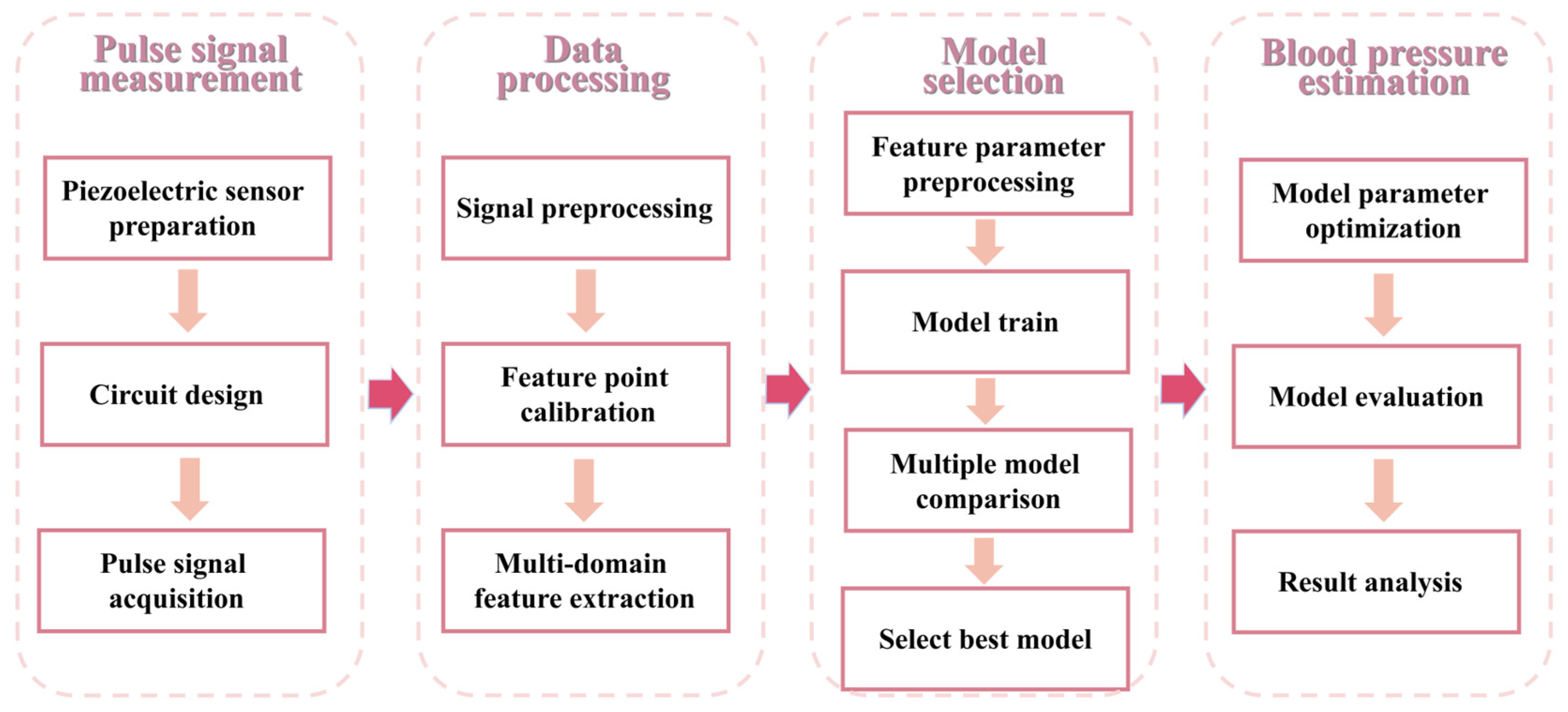
• Construct a variety of machine learning regression models to estimate systolic/diastolic blood pressure, select and optimize the best model and realize the mapping of complex multidimensional pulse wave features to blood pressure values. The research process is shown in Figure 1.

2. Materials and Methods

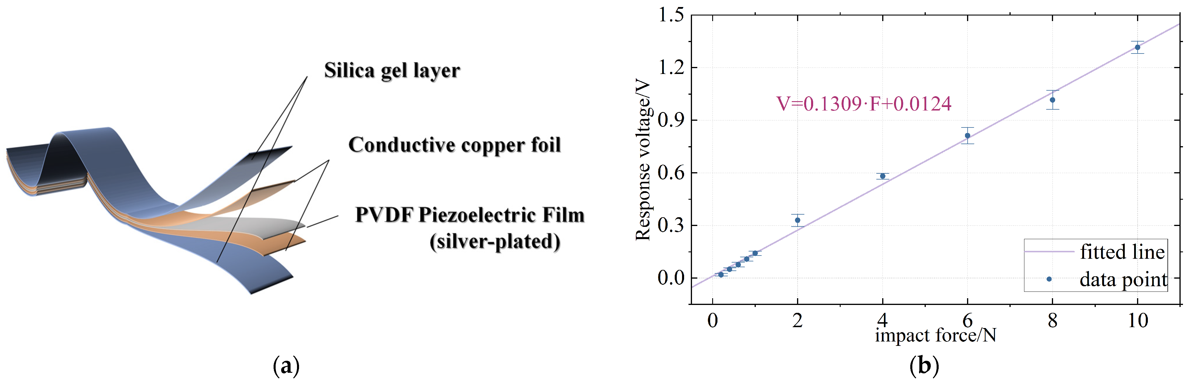
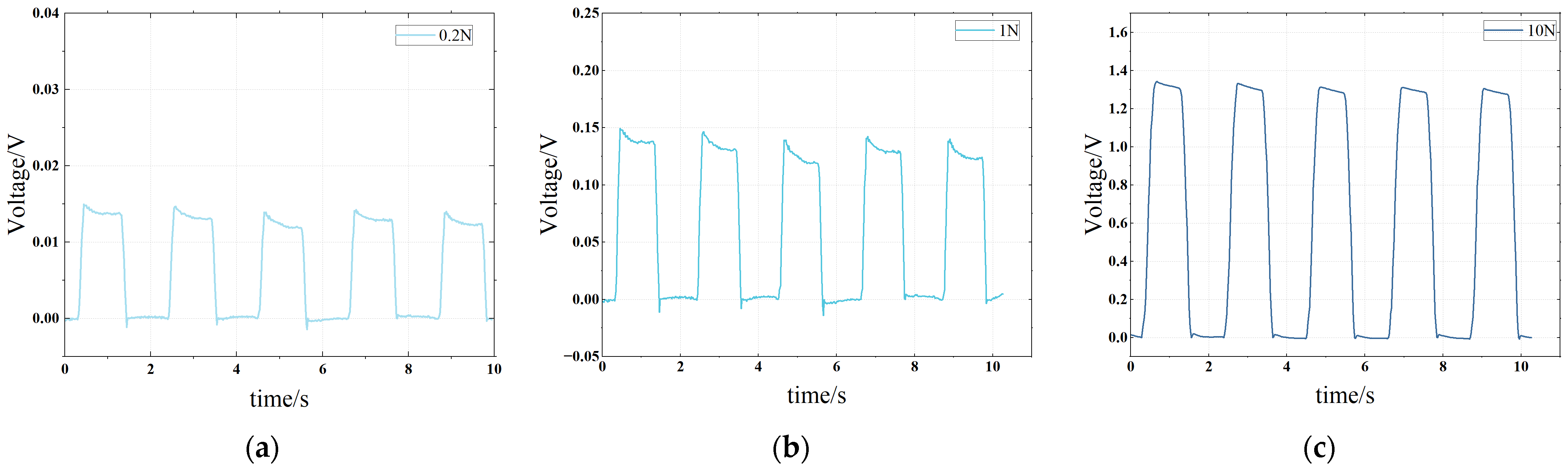
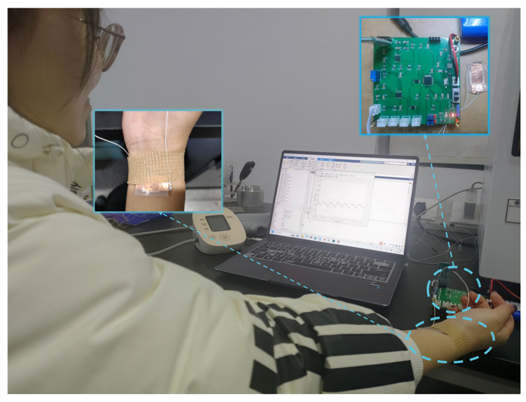
2.1. Preparation of Flexible Pressure Sensor

Pulse wave signals are weak, continuous and complex. Based on the piezoelectric effect, a piezoelectric sensor can convert the impact force and other mechanical signals into voltage signals, and it has the advantages of high sensitivity, fast response and no need for external power supply, so it is suitable for the acquisition of pressure signals with small values [23].

Piezoelectric film based on polyvinylidene fluoride (PVDF) can be used as the sensing material of piezoelectric sensors with high sensitivity and short response time, which is especially suitable for measuring weak body surface signals such as pulse waves [24]. In this paper, a flexible piezoelectric pressure sensor with an appropriate size was developed to record the pulse waveforms of human radial arteries. The specific process is as follows.

First, the PVDF film with an attached silver electrode (l280 mm × 203 mm × 28 µm, Shenzhen Zhimeicong Company, Guangdong, China) was pretreated. It was cut into 10 mm × 10 mm slices. It should be noted that due to the small thickness of the film, direct cutting will lead to the conduction of the silver electrode at the edge. It is necessary to dip a cotton swab into 70% acetone solution and wipe the edge repeatedly until the upper and lower surface resistance is greater than 1 MΩ, measured by a multimeter. At this time, 7 mm × 10 mm of conductive copper foil was cut and pasted on the upper and lower surfaces as electrode leads.

Then, the A and B parts of Ecoflex00-30 (Smooth-On Corporation, USA, for the preparation of a silica gel layer) were poured into a container according to the mass ratio of 1:1 and stirred with a glass rod for 3 min to ensure uniform mixing. At this time, the piezoelectric film was gently placed on the surface of the solution, and the vessel was pumped in a vacuum pump for 10 min to remove bubbles in the mixed liquid and then cured at room temperature for 5 h. At this point, one side of the sensor was packaged. The above steps were repeated to encapsulate the other side. Finally, the excess silica gel was cut off, and the sensor preparation was completed. Its specific structure is shown in Figure 2a.

In order to measure the performance of the flexible piezoelectric sensor, a linear displacement platform (LTS300/M) with an ergometer (Marker 10) was used to apply a fixed value of impact force. At the same time, the piezoelectric sensor was connected to the data acquisition card (National Instruments USB-6210, Austin, TX, USA) and its corresponding response voltage was recorded on LABVIEW. The test conditions are as follows: A metal probe with a diameter of 12 mm was used to apply the impact force at an interval of 1 s. The impact force included a small range 0.2–1 N and a large range 2–10 N. In this paper, the voltage response under different impact forces was measured, and the image was drawn as shown in Figure 2b. It could be seen that the voltage response of the sensor had good linearity. In this paper, the linear relationship is fitted with the first-order function, and the relationship between the force and the corresponding voltage of the piezoelectric sensor is obtained as follows:

$$V=0.1309\cdot F+0.0124$$

(1)

where F is the impact force on the sensor and the unit is N. V is the voltage response of the sensor and the unit is volts. The effect of linear fitting can be evaluated using the determination coefficient $R^2$, which is calculated as follows:

$$R^2=1-{\displaystyle \frac{{\displaystyle \sum _{i=1}^n{\left(y_i-{\widehat{y}}_i\right)}^2}}{{\displaystyle \sum _{i=1}^n{\left(y_i-{\overline{y}}_i\right)}^2}}}$$

(2)

where $y_i$ is the measured value, ${\overline{y}}_i$ is the average value of the measured value, ${\widehat{y}}_i$ is the fitting value and n is the number of data points. The closer $R^2$ is to 1, the better the fit. The piezoelectric sensor $R^2$ of this paper is 0.996, indicating that the voltage response of the sensor has good linearity. In the following measurements, this method is used to calibrate the sensor and convert the measured voltage value to the force value. Since then, this paper generally uses pressure as the unit of pulse signal value, and the corresponding relationship between pressure and force is as follows:

$$p={\displaystyle \frac{F}{S}}$$

(3)

where $F$ is the force on the sensor (unit N), $p$ is the pressure (unit mmHg) and $S$ is the area of the sensor.

Figure 3a–c shows the voltage response of the sensor under three different conditions of 0.2 N, 1 N and 10 N during the experiment. It can be found that the sensor has good consistency in voltage response under forces, which ensures the stable measurement of a pulse wave.

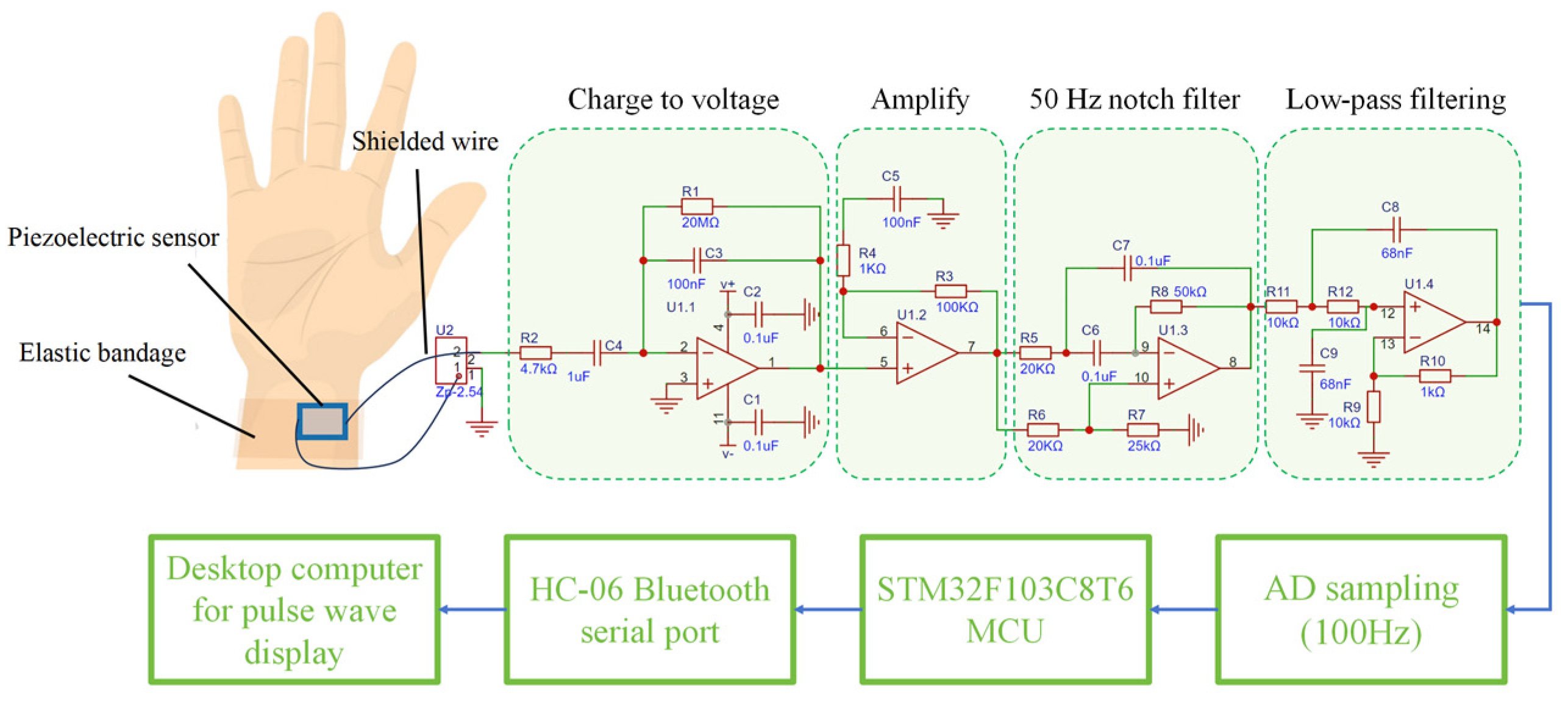
2.2. Measurement System Design

The pulse signal is weak and easy to be disturbed by internal and external noise and the external environment. In addition, the high sensitivity of PVDF piezoelectric film also leads to the poor anti-electromagnetic interference ability of the sensor [25]. Therefore, the signal-conditioning circuit and the corresponding signal acquisition circuit are presented in this paper to collect the pulse signal.

The signal conditioning circuit includes the charge to voltage, voltage amplification, 50 Hz industrial frequency notch and low-pass filtering. The circuit can amplify weaker pulse signals while suppressing 50 Hz industrial frequency noise and other high-frequency interference signals in space. The signal acquisition circuit mainly includes the AD conversion circuit (based on the ADS1115 chip), the STM32F103C8T6 main control chip and the HC-06 Bluetooth module. The signal acquisition circuit can sample the pulse signal at a sampling rate of 100 Hz and transmit it to a computer in the form of a Bluetooth serial port. The structure block diagram of the system is shown in Figure 4.

2.3. Data Acquisition

The pulse wave signal acquisition process mainly involved 45 volunteers in the laboratory team. Of them, 34 were men and 16 were women. All of the study subjects were in good health, did not have cardiovascular disease and had not recently taken medications that affected heart rate or blood vessel tone. All study subjects understood and agreed to participate in this study and signed their informed consent.

Table 1. Basic physiological parameters of the subjects.

Characteristic (Unit)	Mean ± Standard Deviation
Systolic blood pressure (mmHg)	108.4 ± 10.23
Diastolic blood pressure (mmHg)	67.9 ± 10.98
Heart rate (times/minute)	68.8 ± 11.3
Body mass index (kg/m2)	22.6 ± 5.3
Body surface temperature (°C)	35.9 ± 0.53
Age (year)	22.3 ± 5.7

shows the basic physiological parameters and measurement environment of the subjects. The stability of pulse-taking pressure was ensured using medical elastic bandages. The program of the upper computer was written in MATLAB 2020a. The actual measurement scenario is shown in Figure 5.

3. Pulse Signal Processing and Feature Extraction

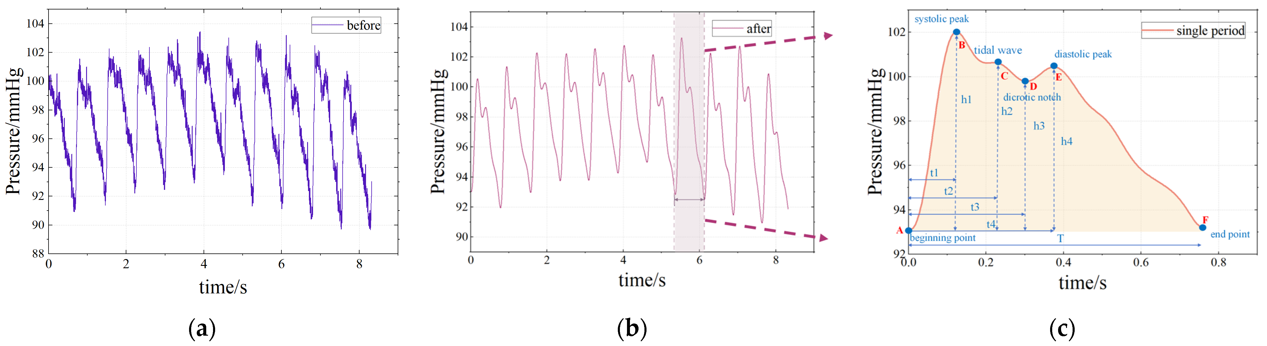
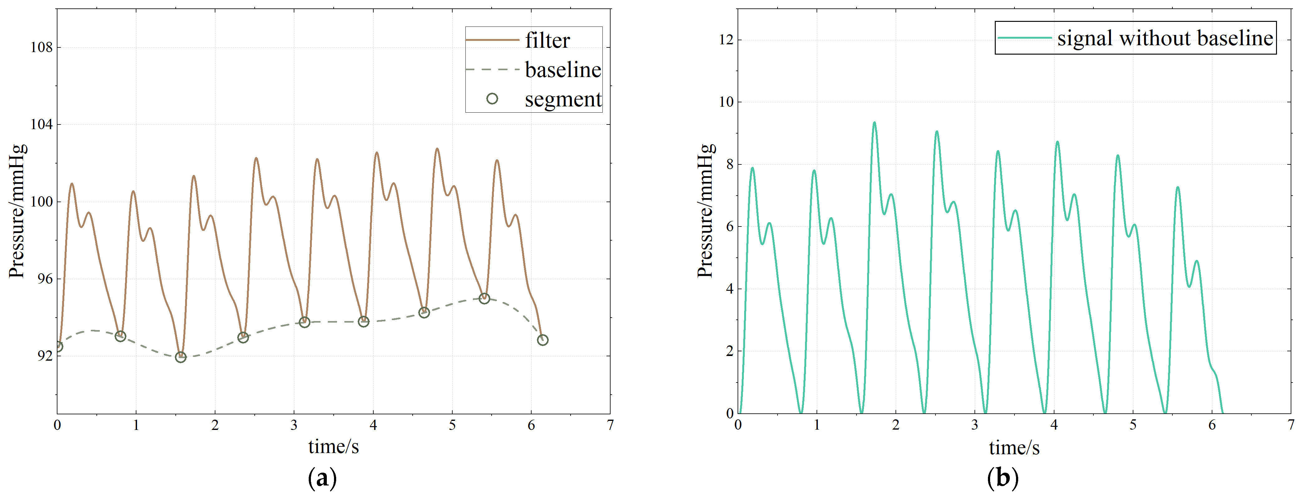
3.1. Signal Preprocessing

A pulse wave is a quasi-periodic low-frequency continuous signal. With changes in the human physiological state and surrounding environment, its waveform also produces subtle changes, so pulse waves have important medical diagnostic significance [26]. The pulse wave signal comes from the beating of the heart, and because the signal source is untouchable, the signal amplitude is small and more susceptible to interference. The pulse wave signal measured with a piezoelectric sensor is mainly subject to interferences including baseline drift, 50 Hz industrial frequency interference and high-frequency interference. Among them, industrial frequency interference, as shown in Section 2.2, was limited by a notch circuit.

The main energy distribution of a pulse wave is in the frequency range of 0–15 Hz [27]. To remove high-frequency interference, the pulse signal is filtered by a 6-order Butterworth filter with a cutoff frequency of 15 Hz. The Butterworth filter has the maximum flat amplitude/frequency response within the passband, that is, there is no ripple in the passband, and it can maintain the original amplitude and shape of the pulse information. In the transition zone, its smooth rolling characteristics make it suitable for the difference in pulse signal frequency distribution of different individuals, and it can better avoid signal distortion. The signal before filtering (the original signal) is shown in Figure 6a, and the signal after filtering is shown in Figure 6b.

In order to explain the formation mechanism and physiological significance of pulse waves, a single period typical pulse wave was intercepted from the continuous pulse wave signal shown in Figure 6b and enlarged to show details, as shown in Figure 6c. The main characteristic points of the waveform mainly include the beginning point A, the systolic peak B, the tidal wave C, the dicrotic notch D, the diastolic peak E and the end point F [27]. The AB segment represents the rapid contractile ejection phase of the ventricle, where arterial pressure rises rapidly. The BD segment represents that the ventricle enters the late systolic period, the ventricular contraction intensity decreases and the dicrotic notch is formed. The DE segment represents the beginning of the ventricular diastole phase when arterial blood volume increases briefly and pressure increases slightly due to valve obstruction. The EF stage means that the left ventricle has fully entered the diastolic phase, the blood in the arterial blood tube flows outwardly, the pressure in the artery decreases and the vessel wall slowly retreats to the initial state. Tidal point C is mainly formed by the characteristics of pulse wave reflection, which is greatly affected by age and individual differences (especially young individuals who are not easy to detect), and is generally not included in the scope of research.

After denoising, a continuous pulse waveform is obtained, as shown in Figure 6b. In order to analyze the characteristics of the pulse wave, it is necessary to perform periodic segmentation, that is, to determine the period segmentation point (A or F) between each single-period pulse waveform. In this paper, a sliding window method is proposed to complete the period segmentation:

First, find the relative minimum points of the continuous pulse signal S1, S2, S3…Sn. Set the signal value of Sn point to S_val. Then, go through each Sn point and determine whether it meets the following two conditions:

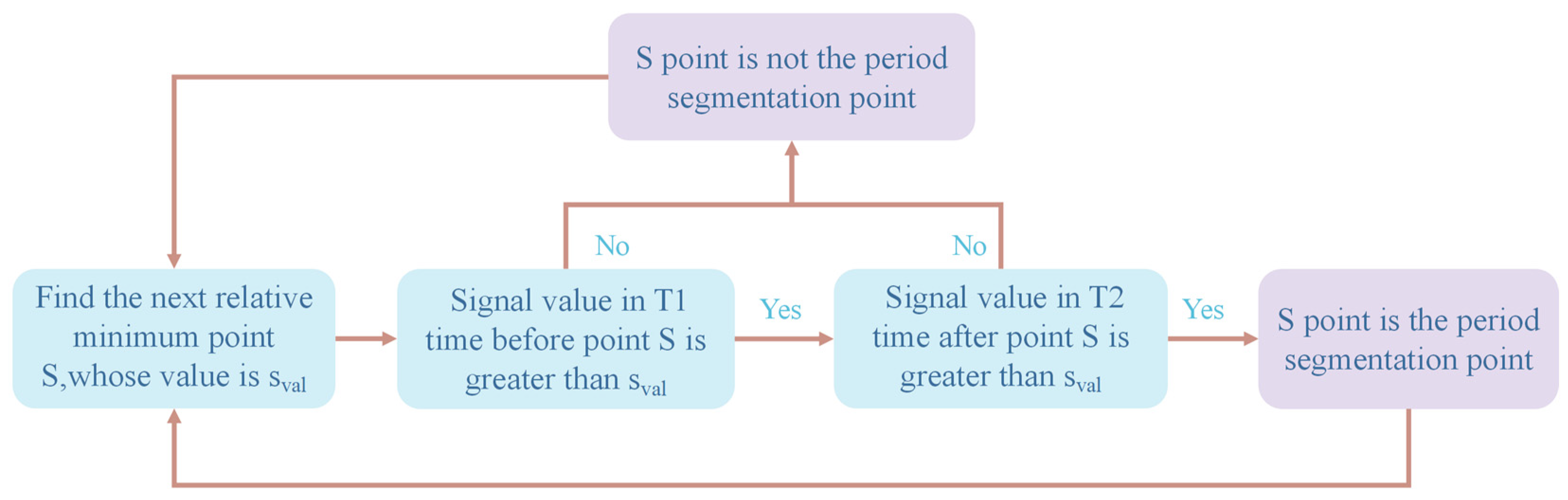
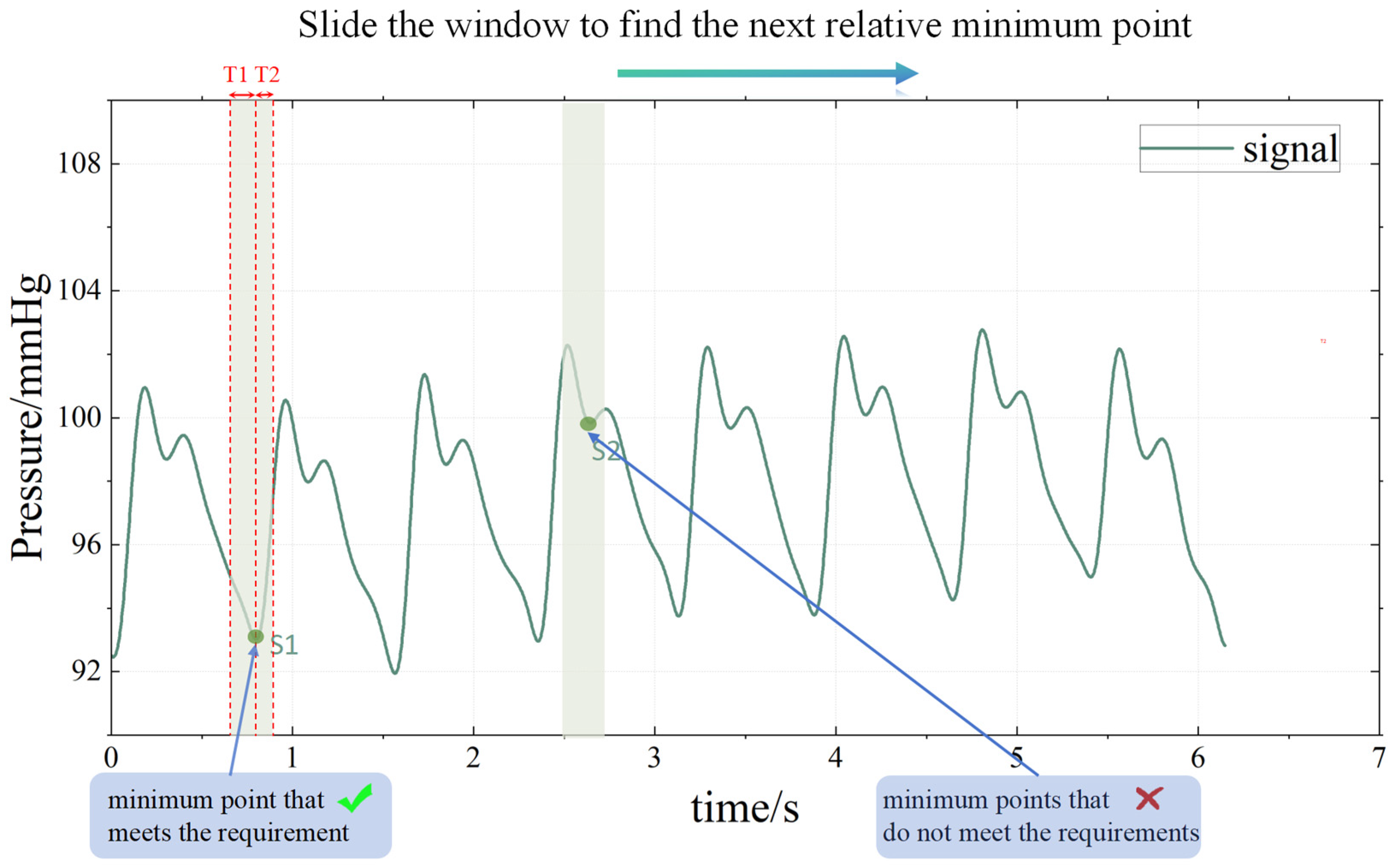
• The signal value of T1 time on the left side of Sn is greater than S_val.
• The signal value of T2 time on the right side of Sn is greater than S_val.

If the above two conditions are met, it means that the Sn point is the periodic segmentation point; otherwise, it is not. This process can be imagined as a time window of length T1 + T2 sliding along the T-axis. Generally, T1 = 0.15 s and T2 = 0.1 s.

The flow chart of this method is shown in Figure 7 and illustrated in Figure 8. This method works well, and the period segmentation points are accurately identified, as shown in the green circle in Figure 9a.

After the period segmentation is completed, the baseline drift problem can be solved. Baseline drift refers to the slow upward or downward movement of the continuous pulse waveform signal in the measurement process, which is mainly caused by human breathing and body displacement in the pulse signal acquisition process, as shown in Figure 9a. The frequency of baseline drift interference caused by human physiological activities generally ranges from 0.05 to 1.5 Hz, and the pulse signal is mainly distributed in the range of 0.7 to 2 Hz. The frequency ranges of the two overlap to a certain extent, so it is difficult to deal with the traditional FIR filter and wavelet transform denoising methods [11,28]. In this paper, spline interpolation is used to deal with the baseline drift. Spline interpolation is a classical curve-fitting method. Here, it fits the periodic segmentation point of the pulse wave as the baseline, obtains the lower envelope of the waveform, and then subtracts the baseline from the original pulse waveform to remove the baseline drift. This method works well in eliminating baseline drift, and the waveform is almost distortion-free, as shown in Figure 9b.

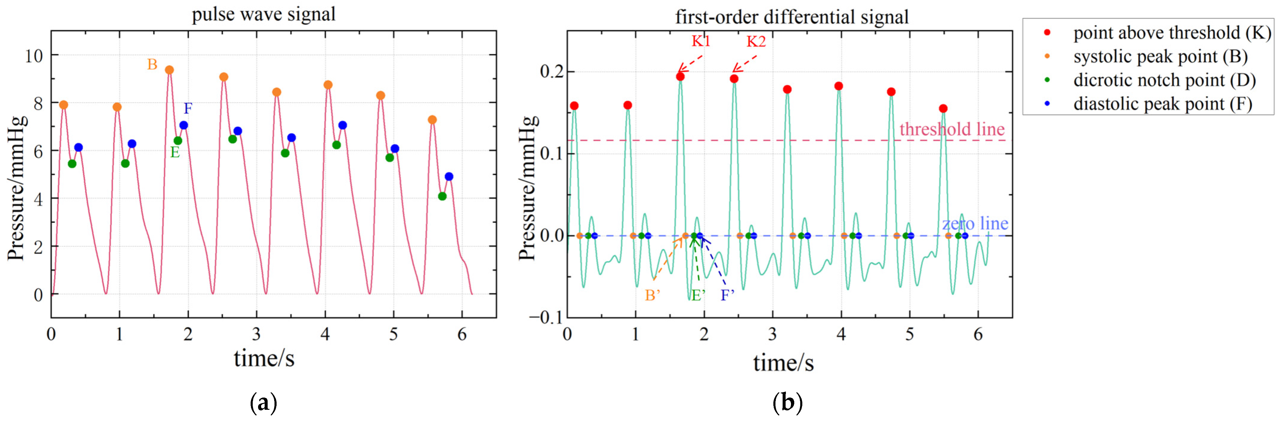
3.2. Pulse Wave Feature Point Calibration

In Section 3.1, segmentation points A and F have been defined. Other feature points B, D and E are identified using the difference threshold method. Set the pulse wave signal as $x\left(n\right)$ and calculate its first-order difference $x_1\left(n\right)$.

The original signal $x\left(n\right)$ is shown in Figure 10a, and the first-order differential signal is shown in Figure 10b. Figure 11 shows the original and first-order differential signals for a pulse period. The meaning of A-F can be seen in Figure 6c.

Finding feature points B, D and E mainly involves the following steps:

Step1. On a first-order differential signal, a threshold line is set that is 0.6 times the global maximum of $x_1\left(n\right)$. This threshold line is shown by the red line in Figure 10.

Step2. Find all the relative maximum points above this threshold line (red dots, e.g., K1, K2).

Step3. Find the zero point between two adjacent relative maximum points (orange dots B’, green dots D’ and blue dots E’ in Figure 10b). These points correspond to points B, D and E on the original signal $x\left(n\right)$, as shown in Figure 10a.

So far, the systolic peak point B, the dicrotic notch point D and the diastolic peak point E have been calibrated.

3.3. Pulse Wave Multi-Domain Feature Extraction

3.3.1. Time Domain Features

After the pulse wave’s feature point is calibrated, its characteristics can be described by t₁, t₃, t₄, T, h₁, h₃, h₄, etc. (tidal wave is not included in the analysis due to its particularity). Definitions of t₁, t₃, t₄, T, h₁, h₃ and h₄ can be seen in Figure 6c. These parameters are the average values of the subjects’ pulse signals within 30 s. Since the pulse wave shape is affected by the pulse-taking pressure and individual differences, the proportional relationship between the parameters can better reflect the physiological condition of the subjects than the absolute amplitude of the wave shape [29]. With reference to Zhang’s research [30], we select the following construction parameters with more physiological significance, as shown in

Table 2. Common construction parameters and physiological significance of pulse waves.

Construction Parameter	Physiological Significance
h3/h1	Reflect the peripheral resistance of aortic wall
h4/h1	Reflect ventricular valve function and aortic compliance
t1/T	Reflect cardiac ejection
t3/t4	Correlate with cardiac fluctuation frequency
Pav	Mean value of arterial pressure (pulse wave)

.

In addition, the pulse area is closely related to the shape of the pulse wave, and the relative area (S_r) and absolute area (S_a) of the waveform are also included in the time domain characteristics. Its calculation formula is as follows:

$$S_r={\displaystyle \frac{{\displaystyle {\int }_0^{\Delta t}x\left(t\right)dt}}{\left[x{\left(t\right)}_{\max }-x{\left(t\right)}_{\min }\right]\cdot \Delta t}}$$

(4)

$$S_a={\displaystyle {\int }_0^{\Delta t}x\left(t\right)dt}-x{\left(t\right)}_{\min }\cdot \Delta t$$

(5)

where $x\left(t\right)$ refers to the pulse signal, $\Delta t$ refers to the duration of the single-period pulse wave and $S_a$ is the yellow part of Figure 6c.

The above 14 features constitute the time domain features of pulse waves.

3.3.2. Frequency Domain Features

The extraction of pulse wave frequency domain features is mainly based on discrete Fourier transform (DFT):

$$X\left(k\right)={\displaystyle \sum _{n=0}^{N-1}x\left(n\right)\cdot e^{-j2\pi kn/N}\hspace{0.33em}\hspace{0.33em}k=0,1\cdots N-1}$$

(6)

where $x\left(n\right)$ is the pulse signal, N is the signal length and $k$ is the frequency. The relationship between pulse wave frequency domain characteristics and human health mainly lies in the distribution of its energy at different frequencies. According to the definition of signal energy, the energy value of the signal at the $k$ frequency component $W\left(k\right)$ is:

$$W\left(k\right)=X^2\left(k\right)$$

(7)

Guo’s related research pointed out that more than 99% of the energy of healthy people’s pulse is distributed within 0–15 Hz. For the unhealthy pulses, such as string pulse and slippery pulse, the pulse energy distribution is more dispersed. For example, in the 0–5 Hz frequency band, the spectral energy of the normal pulse is 90.2%, the spectral energy of the string pulse is 60.9% and the spectral energy of the smooth pulse is 83.7% [27].

Therefore, this paper defines the signal spectral energy ratio SER to describe the cumulative distribution of pulse wave signal energy. SERn represents the proportion of the energy of the signal in the frequency range of 0–n Hz to the total energy of the signal. Its calculation formula is as follows:

$$SERn={\displaystyle \frac{{\displaystyle \sum _{k=0}^{n}W\left(k\right)}}{W_{all}}}$$

(8)

where $W_{all}$ is the total energy of the signal and n is the frequency. For example, SER5 represents the ratio of the signal energy in the frequency range 0–5 Hz to the total energy of the signal. This paper measured SER5, SER10 and SER15 of the volunteers to describe the cumulative energy distribution of the pulse signal at 0–5 Hz, 0–10 Hz and 0–15 Hz, respectively.

In order to describe the distribution characteristics of signal energy, energy entropy (EE) is an important index, reflecting the uniform distribution degree of signal energy in different subintervals. Let the proportion of the energy of frequency $k$ to the total energy be $p_k$, and the energy entropy be:

$$EE=-{\displaystyle \sum _{i=1}^N{p}_i\log p_i}$$

(9)

In addition, the average frequency (F_av) and frequency standard deviation (F_std) of the pulse signal of the person to be measured are also included in the frequency domain features.

The above six features constitute the frequency domain features of pulse waves.

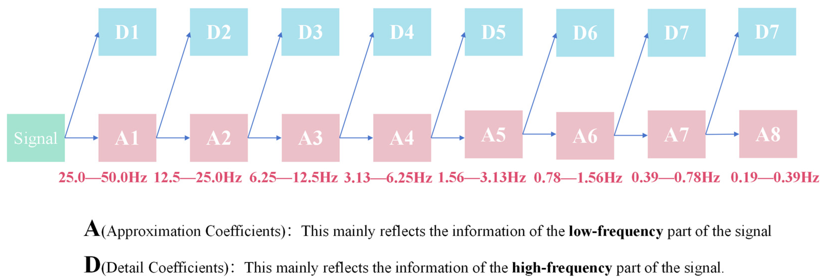
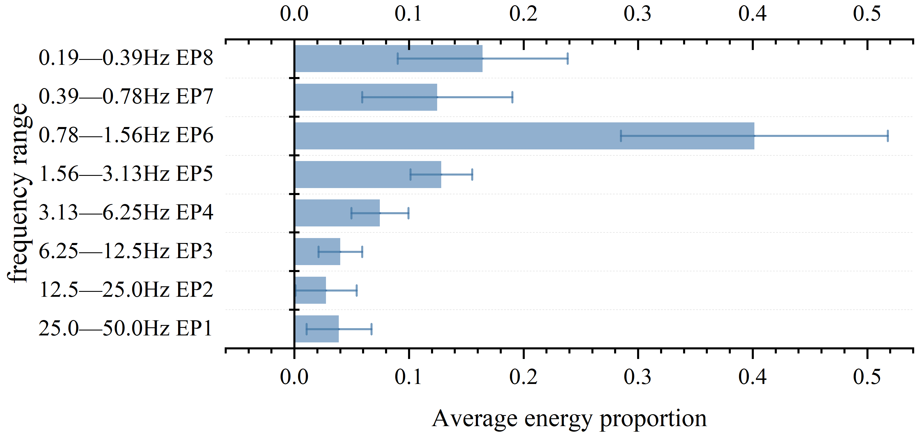
3.3.3. Wavelet Domain Features

The frequency domain feature based on discrete Fourier transform can describe the cumulative distribution of signal energy but its frequency resolution is constant and it is difficult to describe the specific distribution details of the main frequency components of the pulse wave.

Wavelet decomposition is a mathematical tool to decompose a signal into different frequency components, using a wavelet transform to decompose the signal into low-frequency (approximation coefficient) and high-frequency (detail coefficient) parts. Wavelet analysis has the characteristics of multi-resolution, with high time resolution in the high-frequency range and high-frequency resolution in the low-frequency range [31]. Wavelet transform can better display the frequency characteristics of the signal in the low-frequency part, especially suitable for pulse waves with such low-frequency signals.

Because wavelet transform has the advantage of high-frequency resolution in the low-frequency part, sym6 wavelet base pair is used for eight-layer wavelet decomposition. According to the Nyquist sampling theorem and the property of the step-by-step partition of wavelet transform, we divide the signal layer-by-layer from 50 Hz and calculate the sum of squares of the detail coefficients of each layer as the energy of the corresponding frequency band. The idea is shown in Figure 12. Finally, the energy proportion (EP) of each layer after wavelet transformation is selected as the wavelet domain feature of the signal. The EP data for measuring pulse waves in different subjects is shown in Figure 13. It can be found that in the wavelet domain, the pulse signal is mainly distributed in the frequency band of 0.78–1.56 Hz.

It is worth noting that according to the results shown in Figure 13, the values of EP4-EP8 measured in the experiment were 7.5%, 12.8%, 40.1%, 12.5% and 16.4%, respectively. In other words, the energy of the pulse wave in the frequency range of 0.19 Hz to 6.25 Hz accounts for 89.3% of the total energy. This is consistent with the reference value of 90.2% SER5 (0–5 Hz) in healthy people mentioned in the literature [27]. This all proves that the pulse signal of healthy people is mainly concentrated in the low-frequency part. Compared with SERn, which describes the cumulative frequency and energy distribution of 0–n Hz signals, EP obtained with wavelet transform can reflect the specific distribution of pulse signals in different frequency bands, which has positive significance for the construction of the model.

EP1–EP8 are the eight wavelet domain characteristics of pulse waves.

4. Machine Learning Regression

4.1. Model Training and Testing

After completing the above work, we extracted a total of 32 features of pulse waves in the time domain, frequency domain and wavelet domain, as well as the physiological characteristics of the subjects, and recorded them as follows:

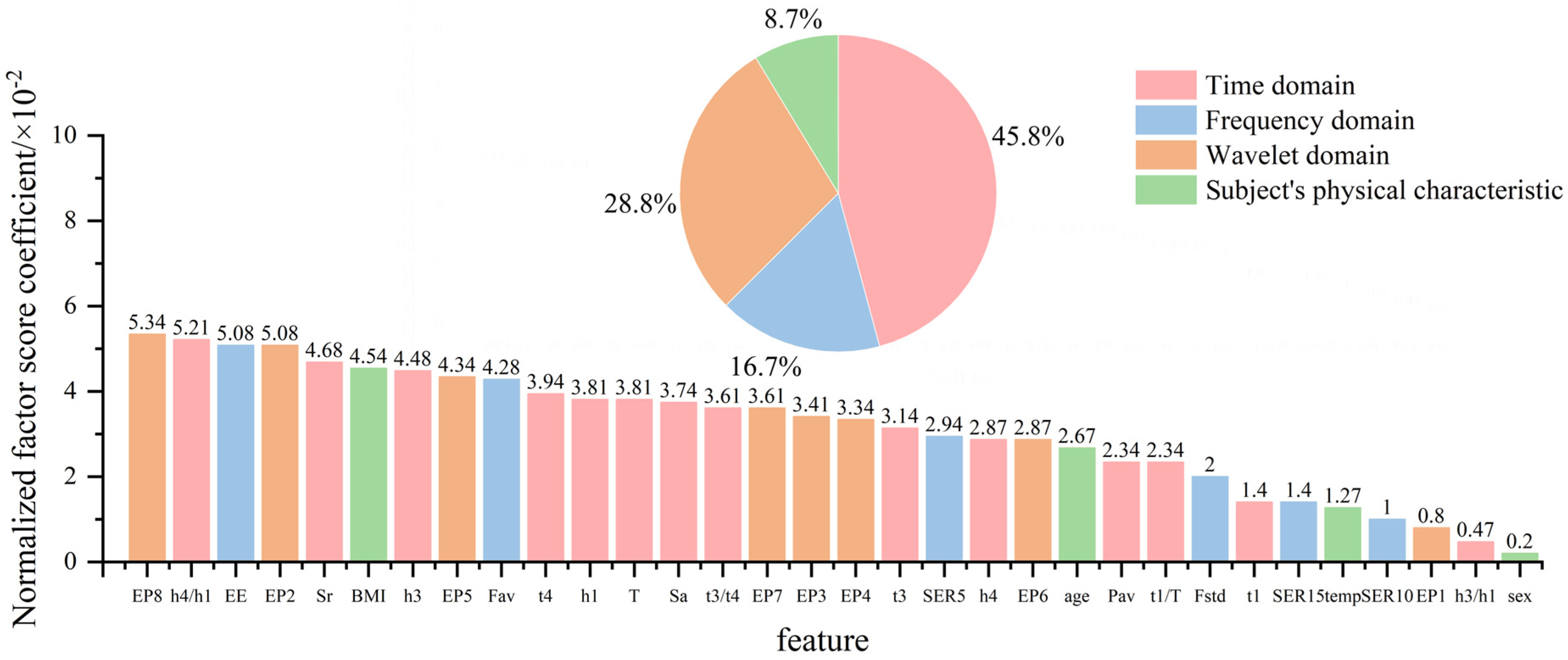
• Time domain features: t₁, t₃, t₄, T, h₁, h₃, h₄, t₁/T, t₃/t₄, h₃/h₁, h₄/h₁, P_av, S_a, S_r.
• Frequency domain features: SER5, SER10, SER15, EE, F_av, F_std.
• Wavelet domain features: EP1–EP8.
• Subjects’ physical characteristics: BMI, body temperature, sex, age.

In order to avoid the difference in feature data dimensions affecting the machine learning regression, we standardized all the data. Where $x$ is the original data, $z$ is the transformed data, $\mu$ is the mean value of the original data and $\sigma$ is the standard deviation of the original data.

$$z={\displaystyle \frac{x-\mu }{\sigma }}$$

(10)

A pulse wave signal is complex and has many features. If these features are mapped to systolic and diastolic blood pressure using a traditional regression model, such as linear regression, it can lead to overfitting because the model tends to remember the noise rather than the true pattern of the extracted data. In order to deal with such problems effectively, it is necessary to adopt regression models that can handle high-dimensional data and have regularization ability. Supervised learning is a method in machine learning that refers to the use of labeled (known inputs and corresponding outputs) training data to train a model so that it can learn the mapping between inputs and outputs and make predictions when it encounters new inputs [32]. Supervised learning methods are widely used in regression tasks. In this paper, the 30 features mentioned above are used as labels to train the supervised learning model and map the 30 features of pulse waves to the two indexes of systolic blood pressure (SBP) and diastolic blood pressure (DBP).

In terms of model selection, we focused on models that can handle high-dimensional complex data, and selected five supervised learning models with different characteristics: typical neural network model multi-layer perceptron, non-parametric model K-nearest neighbor network regression (KNN), integrated model random forest regression, improved linear model elastic network regression and statistical model Bayesian regression. When building the machine learning model, 45 subjects were randomly divided into a training set of 27 and a test set of 18. Random division ensures the balance of data distribution and improves the generalization ability of the model.

In this paper, the systolic and diastolic blood pressures measured using Omron sphygmomanometer were used as the standard reference values. The relationship between the estimated value and the reference value is plotted as shown in Figure 14. The distribution of scatter points in the figure represents the relationship between the estimated value and the reference value. The closer the scatter point is to the y = x line, the more the estimated value and reference value tend to be consistent, indicating that the model has a better estimation effect.

In order to visually compare the regression effects of each model, RMSE (mean square error), MAE (mean absolute error), MAPE (mean absolute percentage error) and R² (determination coefficient) between the estimate and the reference value were calculated to evaluate the performance of the regression model. RMSE gives more weight to large errors, MAE gives equal weight to all errors and MAPE indicates the percentage of error relative to the actual value. R² is used to measure the degree to which the regression model explains the dependent variable. The closer to 1, the better the regression effect. The calculation formula is as follows:

$$RMSE=\sqrt{{\displaystyle \frac{1}{n}}{\displaystyle \sum _{i=1}^n{\left(y_i-{\widehat{y}}_i\right)}^2}}$$

(11)

$$MAE={\displaystyle \frac{1}{n}}{\displaystyle \sum _{i=1}^n\left|y_i-{\widehat{y}}_i\right|}$$

(12)

$$MAPE={\displaystyle \frac{1}{n}}{\displaystyle \sum _{i=1}^n\left|\frac{y_i-{\widehat{y}}_i}{y_i}\right|}\times 100\%$$

(13)

$$R^2=1-{\displaystyle \frac{{\displaystyle \sum _{i=1}^n{\left(y_i-{\widehat{y}}_i\right)}^2}}{{\displaystyle \sum _{i=1}^n{\left(y_i-{\overline{y}}_i\right)}^2}}}$$

(14)

where $y_i$ is the reference value (actual value), ${\widehat{y}}_i$ is the estimated value, ${\overline{y}}_i$ is the average value of estimated value and n is the number of data points. The smaller the error, the better the regression effect. The RMSE, MAE, MAPE, R² and training time estimated by the five models for systolic blood pressure (SBP) and diastolic blood pressure (DBP) are shown in

Table 3. The error and training duration of SBP and DBP were estimated by five regression models.

Machine Learning Model		RMSE	MAE	MAPE	R2	Training Duration
Multilayer perceptron	SBP	4.800	3.960	3.58%	0.741	0.109 s
	DBP	2.739	2.073	2.99%	0.855	0.109 s
K-nearest neighbor network regression	SBP	7.582	6.122	5.50%	0.208	0.002 s
	DBP	5.222	4.357	5.73%	0.161	0.002 s
Random forest regression	SBP	3.077	2.719	2.49%	0.881	0.057 s
	DBP	2.058	1.628	2.10%	0.896	0.055 s
Elastic network regression	SBP	3.357	2.981	2.67%	0.847	0.102 s
	DBP	2.477	1.823	2.37%	0.879	0.100 s
Bayesian regression	SBP	7.589	5.926	5.20%	0.294	0.027 s
	DBP	5.670	4.596	5.97%	0.273	0.016 s

. Numerical visualization is shown in Figure 15.

The multi-layer perceptron model (MLP) has good nonlinear modeling ability and is good at dealing with nonlinear mapping, which is suitable for complex regression tasks. As can be seen from Figure 14 and Figure 15, the mean percentage error (MAPE) of MLP regression in estimating systolic and diastolic blood pressure was 3.58% and 2.99%, respectively. The regression effect is not very ideal. This may be due to the sensitivity of the MLP model to data size and data distribution. When the data scale is not large enough and contains some abnormal data, it is difficult for the model to learn a stable mapping relationship. MLP regression is particularly sensitive to model parameters and is prone to overfitting or inadequate generalization.

K-nearest neighbor network model (KNN) is a lazy learning algorithm that does not perform explicit training but calculates the similarity between samples when making predictions. The MAPE of KNN regression in estimating systolic and diastolic blood pressure was 5.50% and 5.73%, respectively, with poor results. This is mainly due to the instability of thee KNN algorithm on high-dimensional data. Pulse wave data have 32 characteristics, which is typical of high-dimensional data. As a result, the distance between samples tends to be similar, and KNN can hardly find effective adjacent samples, which affects the prediction accuracy.

The elastic net model (EN) is an improved linear regression model that can automatically select features and has good robustness. EN regression estimated the MAPE of systolic and diastolic blood pressure to be 2.67% and 2.37%, respectively. This shows the applicability of elastic network regression to high-dimensional data, and that it performs better on data with a much larger number of features than the number of samples and can avoid the overfitting problem of ordinary linear regression. However, the elastic network model is a linear model in nature, the regression result process is difficult to explain and the training time is long.

The Bayesian model (BYS) is a probabilistic modeling model that uses probabilistic operations to make predictions. BYS regression estimated the MAPE of systolic and diastolic blood pressure to be 5.20% and 5.97%, respectively, with poor results. Bayesian regression usually assumes that the error follows a normal distribution, and a complex signal such as a pulse wave does not conform to the general probability relationship, which may affect the fitting effect.

The random forest model (RF) is an ensemble learning method that builds multiple decision trees and averages them to obtain a final prediction. The model has good nonlinear modeling ability, is robust to outliers and noise and has low requirements on a data scale. RF regression estimated the MAPE of systolic and diastolic blood pressure to be 2.49% and 2.10%, respectively. According to the Association for the Advancement of Medical Instrumentation (AAMI) criteria, the mean absolute error (MAE) of measuring (or estimating) blood pressure should not exceed ±5 mmHg. The MAEs of random forest regression on systolic blood pressure and diastolic blood pressure were 2.72 mmHg and 1.63 mmHg, respectively, showing good robustness and fewer errors than other models. The regression results show that the random forest model can capture the relationship between the complex pulse wave signal and systolic/diastolic blood pressure, and effectively deal with the nonlinear mapping relationship. Therefore, we chose the random forest regression model for further optimization.

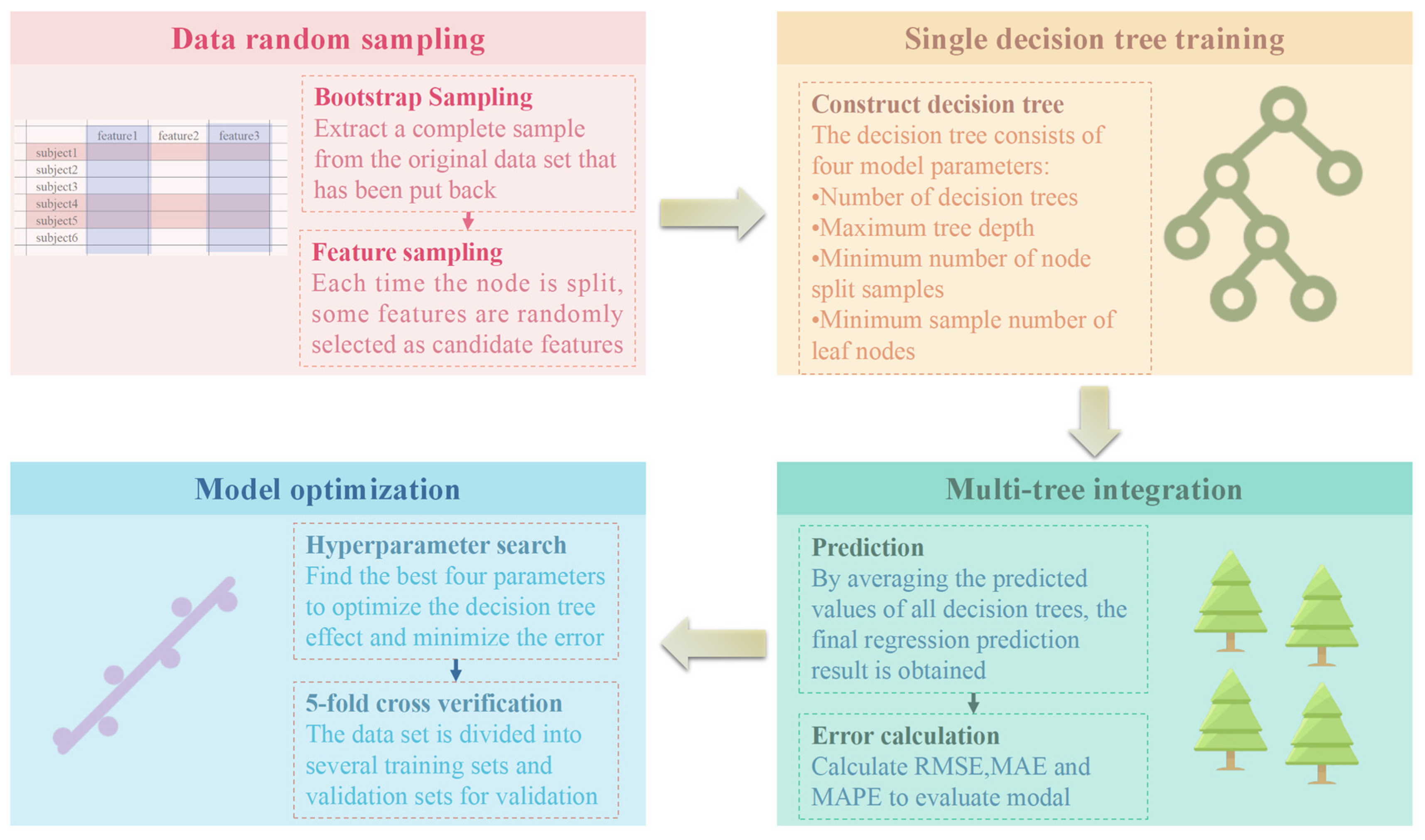
4.2. Model Optimization

The random forest algorithm is a powerful machine learning technique that can effectively model nonlinear relationships and handle small samples. Some studies have emphasized that the random following forest algorithm can model complex relationships in data with limited observational data [33]. It has been noted that random forests “can easily accommodate missing values, nonlinear relationships, interactions, and a large number of covariables” [34]. This makes random forest regression more suitable for non-invasive blood pressure estimation using pulse waves to obtain this nonlinear relationship.

Random forest (RF) is an integrated learning method based on decision trees. By constructing multiple independent decision trees and averaging the final regression results, the generalization ability and stability of the model are improved. The construction of a random forest consists of the following key steps [35]:

1. Bootstrap sampling: random sampling with return is performed from the original training data set to generate multiple sub-data sets, and each data set is used to train a decision tree.

2. Random selection of features: In the node-splitting process of each decision tree, not all features are divided, but some features are randomly selected for the best division. This increases the diversity between trees and reduces the risk of overfitting.

3. Multi-tree integration: The final model combines the prediction results of all decision trees. For regression tasks, the mean value of all decision tree output values is usually used as the final regression value. This can reduce the variance of a single decision tree and improve the stability of the model.

In this study, the process of random forest model construction is shown in Figure 16.

In machine learning, a hyperparameter is a parameter that can be set to define any configurable part of the model learning process. A hyperparameter search is a method to select an optimal set of hyperparameters for a learning algorithm [36,37]. In order to improve the accuracy of blood pressure estimation, this paper optimized the following four hyperparameters of the random following forest model:

• Number of decision trees: a reasonable choice of this parameter can strike a balance between model complexity and computational efficiency.
• Maximum tree depth: reasonable parameters can avoid underfitting and overfitting.
• Minimum number of node split samples: a smaller value will make the tree grow deeper, while a larger value will limit the tree’s growth and reduce the risk of overfitting.
• Minimum sample number of leaf nodes: a small value may lead to an increase in the number of leaf nodes, making the model more flexible but easy to overfit, while a larger value will enhance the regularization ability of the model and improve the generalization performance [38].

In this paper, a model was constructed based on PYTHON’s RandomForestRegressor library, and the optimal hyperparameters for the model were determined by means of a grid search and then cross-validated 5-fold. It was necessary to find the best balance between model complexity and generalization ability to improve the accuracy of systolic/diastolic blood pressure estimation with pulse wave features. Finally, the number of decision trees of the model was determined to be 130, the maximum depth is 10, the minimum number of node split samples is 2 and the minimum number of leaf nodes is 1. After optimization, the MAE of systolic blood pressure estimation is 1.72 mmHg and the MAPE is 1.55%; the MAE of diastolic blood pressure estimation is 1.40 mmHg and the MAPE is 1.8%. The visualization of the specific results is shown in Figure 17.

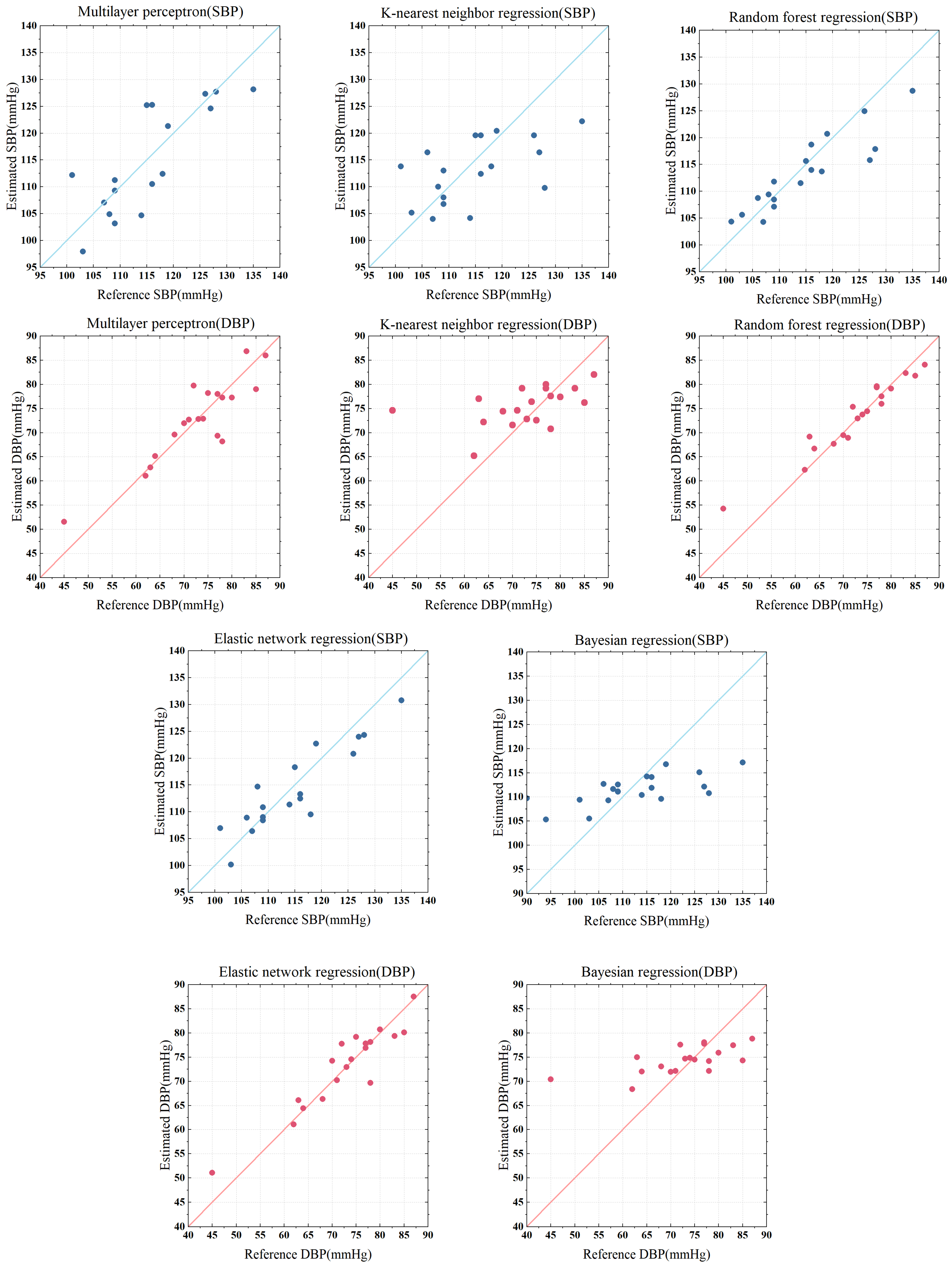
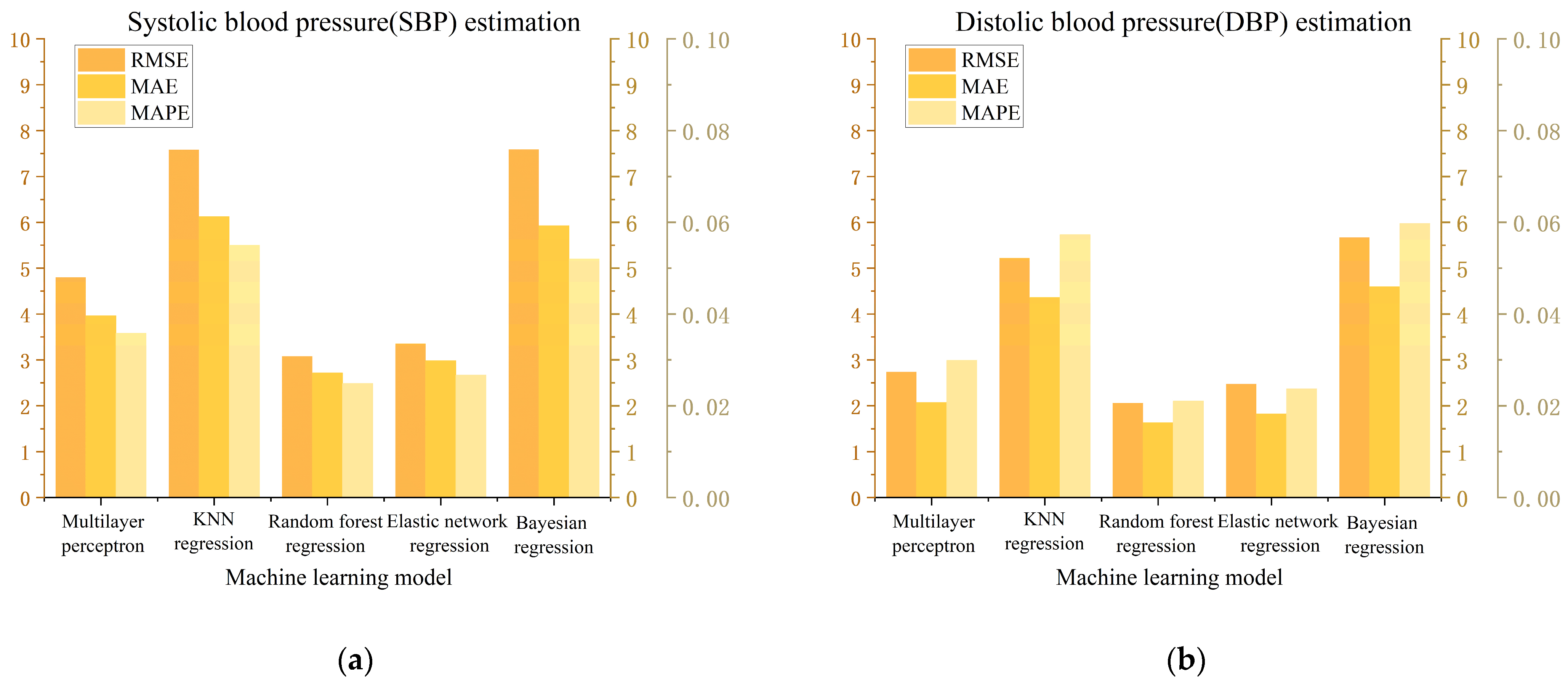
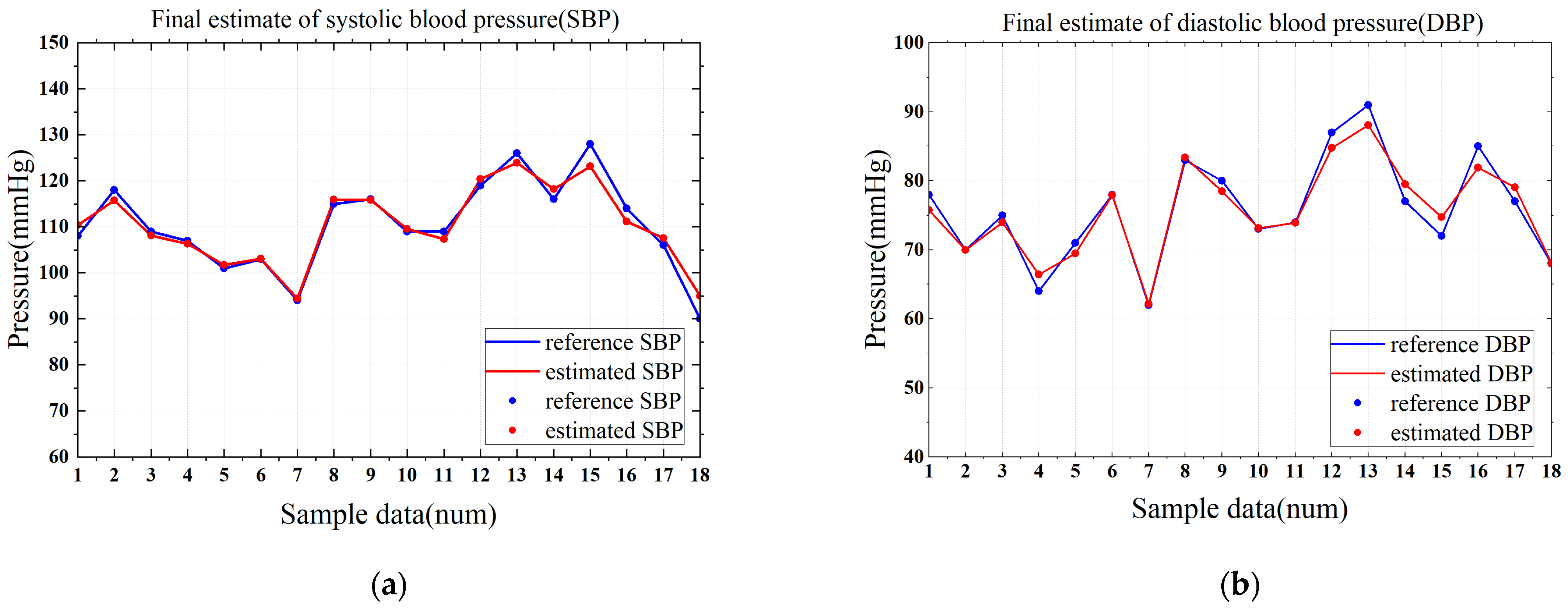
4.3. Result Analysis

After the random forest model completes the regression, it can also obtain the importance degree for each feature. Random forests assess the importance of features by calculating how much the features affect the model estimates. During the construction of the decision tree, each feature is used to split the data to reduce impurity (such as information entropy or mean square error).

The sum of the impurity reduction of each feature on all trees is calculated to obtain the normalized feature importance. The importance of features can help us judge the correlation between different pulse wave signs and blood pressure and can reflect the contribution of features in blood pressure estimation. The importance of the 32 features is shown in Figure 18.

As can be seen from Figure 18, time domain features contribute the most to the estimation of blood pressure. In particular, the representative features of the diastolic branch of a pulse wave, such as h₄/h₁, h₃, t₃/t₄, t₃, t₄, etc., accounted for 6.1%, 5.56%, 4.71%, 4.1% and 4.07%, respectively, indicating that the diastolic period of a pulse wave is closely related to the blood pressure value. From the frequency domain, pulse energy entropy (EE) makes the largest contribution to the estimation of blood pressure, accounting for 8.6%, while SERn, which describes the cumulative distribution of pulse energy in the frequency domain, makes little contribution. This highlights that in the frequency domain, the distribution of pulse energy can better map blood pressure information, rather than cumulative conditions. In the wavelet domain, the contribution of EPn is more balanced, which highlights the complexity of pulse signals, indicating that blood pressure information is more determined by the distribution of energy in each frequency band rather than the information of a certain frequency band. The overall contribution of the subjects’ physiological status (BMI and body temperature) is only 7.5%, which indicates that the model has a good generalization ability and is not affected by individual differences. Among them, BMI affects the pulse-taking pressure, which also has a certain impact on the shape of pulse signals.

To verify the above results, principal component analysis (PCA) was used to verify the importance of each feature. PCA is a dimensionality reduction method that projects high-dimensional data into a new low-dimensional space by linear transformation while retaining variance information of the original data as much as possible. In this paper, a PCA method is used to reduce the dimensions of 32 features into a one-dimensional F1. The contribution of the feature to the principal component F1 is judged by the factor score coefficient of the feature. The calculation formula is as follows:

$$F1={\displaystyle \sum _{i=1}^{32}{w}_i\cdot X_i}$$

(15)

where $w_i$ is the factor score coefficient and $X_i$ is the feature. The greater the absolute value of the factor score coefficient, the greater the contribution of the feature to the principal component and the more important the feature. In order to measure the importance of the features, this paper takes the absolute value of the factor score coefficient.

After the factor score coefficient is standardized, it is shown in Figure 19. Comparing Figure 18 and Figure 19, it can be found that the features that contribute more to the random forest model have relatively high factor score coefficients. For example, the contribution of the time domain features is more than 40%, and the proportion of the wavelet domain features is close to 30%, indicating that they contain more physiological information. This verifies the conclusion of this paper. There is also a slight difference between Figure 18 and Figure 19, which is due to the fact that PCA does not correlate the features with blood pressure but rather in terms of how much information the features themselves contain.

5. Conclusions

A blood pressure estimation system based on pulse waves is presented in this paper that can be used for simple and reliable daily blood pressure monitoring. By designing a flexible piezoelectric sensor and its supporting circuit, we can capture pulse waveforms stably. This study also designed a complete pulse signal processing method, including filtering, baseline drift and feature point calibration. Thirty features were extracted from the time domain, frequency domain and wavelet domain of the pulse signal for training the machine learning regression model. Finally, it can be determined that the random forest model has higher accuracy and a lower training cost and can better estimate systolic/diastolic blood pressure using pulse wave signs. In addition, it can be found that the diastolic features of pulse waves and the distribution of energy in low-frequency bands may contribute significantly to the estimation of blood pressure under the random forest model. The experimental results show that the mean absolute error of systolic blood pressure and diastolic blood pressure measured by our system is 1.72 mmHg and 1.40 mmHg, which meets the requirement of the AAMI standard that the mean absolute error is less than 5 mmHg. In the future, it may be possible to complete the entire system with the integration of multiple machine learning models to improve the accuracy of estimates. Overall, this study developed a complete blood pressure estimation system based on the pulse wave method. The measurement method is intuitive and simple, with qualified accuracy, and is expected to be applied in long-term daily blood pressure monitoring.

References

1. Thomas, B.; Gabriele, K.K.; Gaia, K.; Harsha, M.; Markus, S.; Aletta, E.; George, S.S.; Ji, G.W.; Marcos, J.M.; Rafael, H.H.; et al. May Measurement Month 2022: Results from the global blood pressure screening campaign. BMJ Glob. Health 2024, 9, e016557. [Google Scholar]
2. Sliwa, K.; Ojji, D.; Bachelier, K.; Böhm, M.; Damasceno, A.; Stewart, S. Hypertension and hypertensive heart disease in African women. Clin. Res. Cardiol. 2014, 103, 515–523. [Google Scholar] [PubMed]
3. Stantliff, T.M.; Salindri, A.D.; Egoavil, E.R. Abnormal blood pressure among individuals evaluated for tuberculosis infection in a U.S. public health tuberculosis clinic. Epidemiol. Infect. 2024, 152, 133. [Google Scholar]
4. Kang, W.; Pineda Hernández, S. Understanding Cognitive Deficits in People with High Blood Pressure. J. Pers. Med. 2023, 13, 1592. [Google Scholar] [CrossRef]
5. Lurbe, E.; Mancia, G.; Calpe, J. Joint statement for assessing and managing high blood pressure in children and adolescents: Chapter 1. How to correctly measure blood pressure in children and adolescents. Front. Pediatr. 2023, 11, 40–57. [Google Scholar]
6. Jiang, Z.; Li, S.; Wang, L. A comparison of invasive arterial blood pressure measurement with oscillometric non-invasive blood pressure measurement in patients with sepsis. J. Anesth. 2024, 38, 222–231. [Google Scholar]
7. Diaz, A.; Zócalo, Y.; Salazar, F.; Bia, D. Non-invasive central aortic pressure measurement: What limits its application in clinical practice? Front. Cardiovasc. Med. 2023, 10, 43–59. [Google Scholar]
8. Bogatu, L.I.; Turco, S.; Mischi, M.; Muehlsteff, J.; Woerlee, P. An Experimental Study on the Blood Pressure Cuff as a Transducer for Oscillometric Blood Pressure Measurements. IEEE Trans. Instrum. Meas. 2021, 70, 1–11. [Google Scholar]
9. Marks, L.A.; Groch, A. Optimizing cuff width for noninvasive measurement of blood pressure. Blood Press. Monit. 2000, 5, 153–158. [Google Scholar]
10. Celler, B.G.; Yong, A.; Rubenis, I.; Butlin, M.; Argha, A.; Rehan, R.; Avolio, A. Evaluation of the oscillometric method for noninvasive blood pressure measurement during cuff deflation and cuff inflation with reference to intra-arterial blood pressure. J. Hypertens. 2024, 42, 1235–1247. [Google Scholar]
11. Zhang, Y.F. Research on Pulse Signal Acquisition and Analysis Based on Piezoelectric Sensing. Master’s Thesis, South China University of Technology, Guangzhou, China, 2023. [Google Scholar]
12. Yuan, B. Design of blood pressure measurement system based on pulse wave conduction time. Digit. Technol. Appl. 2016, 10, 159. [Google Scholar]
13. Yao, Y.; Zhou, S.; Alastruey, J.; Hao, L.; Greenwald, S.E.; Zhang, Y.; Xu, L.; Xu, L.; Yao, Y. Estimation of central pulse wave velocity from radial pulse wave analysis. Comput. Methods Programs Biomed. 2022, 219, 17. [Google Scholar]
14. Yi, Z.; Liu, Z.; Li, W.; Ruan, T.; Chen, X.; Liu, J.; Yang, B.; Zhang, W. Piezoelectric Dynamics of Arterial Pulse for Wearable Continuous Blood Pressure Monitoring. Adv. Mater. 2022, 34, 16–27. [Google Scholar]
15. Andreozzi, E.; Sabbadini, R.; Centracchio, J.; Bifulco, P.; Irace, A.; Breglio, G.; Riccio, M. Multimodal Finger Pulse Wave Sensing: Comparison of Forcecardiography and Photoplethysmography Sensors. Sensors 2022, 22, 7566. [Google Scholar] [CrossRef] [PubMed]
16. Lin, S.-T.; Chen, W.-H.; Lin, Y.-H. A Pulse Rate Detection Method for Mouse Application Based on Multi-PPG. Sensors. Sensors 2017, 17, 1628. [Google Scholar] [CrossRef]
17. Li, Q.L. Research on Tactile Type Recognition Based on Piezoelectric Film Sensor. Master’s Thesis, Jilin University, Changchun, China, 2024. [Google Scholar]
18. Li, H.B. Performance Optimization and Embedded Design Development of PVDF Flexible Piezoelectric Films. Master’s Thesis, Henan University, Zhengzhou, China, 2023. [Google Scholar]
19. Zhu, Z.M. Research on Multi-Frequency Domain Multi-Feature Identity Recognition Method and System Based on PPG and ECG Signals. Master’s Thesis, Nanjing University of Posts and Telecommunications, Nanjing, China, 2023. [Google Scholar]
20. Tian, S.; Wang, L.; Zhu, R. A flexible multimodal pulse sensor for wearable continuous blood pressure monitoring. Mater. Horiz. 2024, 11, 2428–2437. [Google Scholar] [PubMed]
21. Wang, X.; Wu, G.; Zhang, Z. Traditional Chinese Medicine (TCM)-Inspired Fully Printed Soft Pressure Sensor Array with Self-Adaptive Pressurization for Highly Reliable Individualized Long-Term Pulse Diagnostics. Adv. Mater. 2024, 10, 241–254. [Google Scholar]
22. Mou, H.; Yu, J. CNN-LSTM Prediction Method for Blood Pressure Based on Pulse Wave. Electronics 2021, 10, 1664. [Google Scholar] [CrossRef]
23. Gu, J.; Xu, S.D.; Lu, X.L. Study on the membrane formation mechanism of PVDF/PVDF-CTFE blends. J. Taiwan Inst. Chem. Eng. 2023, 142, 1070–1076. [Google Scholar]
24. Zou, D.; Xia, L.B.; Luo, P.; Guan, K.C.; Hideto, M.; Zhong, Z.X. Fabrication of hydrophobic bi-layer fiber-aligned PVDF/PVDF-PSF membranes using green solvent for membrane distillation. Desalination 2023, 565, 64–81. [Google Scholar]
25. Cao, C.J.; Lai, K.X.; Wang, X.S. Design of wearable pulse sensor based on flexible piezoelectric film. J. Electron. Meas. Instrum. 2012, 38, 35–47. [Google Scholar]
26. Wang, T.W.; Lin, S.F. Wearable Piezoelectric-Based System for Continuous Beat-to-Beat Blood Pressure Measurement. Sensors 2020, 20, 851. [Google Scholar] [CrossRef] [PubMed]
27. Guo, B. Pulse Detection System Based on Flexible Pressure Sensor. Master’s Thesis, Nanjing University, Nanjing, China, 2021. [Google Scholar]
28. Wang, R.; Li, J.; Wang, H.; Deng, S.; He, C.; Miljevic, B.; Ristovski, Z.; Wang, B. Development and Validation of the Particle into Nitroxide Quencher System with BPEAnit Probe for High-Sensitivity Reactive Oxygen Species Detection in Atmospheric Monitoring. Sensors 2025, 25, 1129. [Google Scholar] [CrossRef]
29. Dong, X.H. Study on the Influence Mechanism of Controlled Contact Pressure on Pulse Wave Signal of Photoelectric Volume. Master’s Thesis, Guilin University of Electronic Technology, Guilin, China, 2023. [Google Scholar]
30. Zhang, Y.L. Research on Flexible Pressure Sensor Array for Pulse Detection. Master’s Thesis, Soochow University, Suzhou, China, 2020. [Google Scholar]
31. Tian, C.W.; Zheng, M.H.; Zuo, W.M.; Zhang, B.; Zhang, Y.N.; Zhang, D. Multi-stage image denoising with the wavelet transform. Pattern Recognit. 2023, 134, 109050. [Google Scholar] [CrossRef]
32. Van Engelen, J.E.; Hoos, H.H. A survey on semi-supervised learning. Mach. Learn. 2020, 109, 373–440. [Google Scholar]
33. McAlexander, R.J.; Mentch, L. Predictive inference with random forests: A new perspective on classical analyses. Res. Politics 2020, 7, 20–56. [Google Scholar] [CrossRef]
34. Tudor, C.; Sova, R.; Stamatiou, P.; Vlachos, V.; Polychronidou, P. Future-Proofing EU-27 Energy Policies with AI: Analyzing and Forecasting Fossil Fuel Trends. Electronics 2025, 14, 631. [Google Scholar] [CrossRef]
35. Daniel, B.; Bent, J.C.; Nicolaj, S.M.; Mikkel, S.N. Targeting predictors in random forest regression. Int. J. Forecast. 2023, 39, 841–868. [Google Scholar]
36. Mizumoto, A. Calculating the relative importance of multiple regression predictor variables using dominance analysis and random forests. Lang. Learn. 2022, 73, 161–196. [Google Scholar] [CrossRef]
37. Yi, L.; Zou, C.; Berecibar, M.; Nanini-Maury, E.; Chan, J.C.; Van den Bossche, P.; Van Mierlo, J.; Omar, N. Random Forest regression for online capacity estimation of lithium-ion batteries. Appl. Energy 2018, 232, 197–210. [Google Scholar]
38. Ali, N.; Chen, J.; Fu, X.; Ali, R.; Hussain, M.A.; Daud, H.; Hussain, J.; Altalbe, A. Integrating Machine Learning Ensembles for Landslide Susceptibility Mapping in Northern Pakistan. Remote Sens. 2024, 16, 988. [Google Scholar] [CrossRef]
Figure 1. Overall study flow chart of the proposed non-invasive blood pressure estimation.
Electronics 14 01409 g001
Figure 2. Structure and characteristics of piezoelectric sensors. (a) Structure of piezoelectric sensor. (b) The response voltage of piezoelectric sensor varies with force.
Electronics 14 01409 g002
Figure 3. Voltage response of piezoelectric sensor under different impact forces. (a) The impact force is 0.2 N, and the interval is 1 s. (b) The impact force is 1 N, and the interval is 1 s. (c) The impact force is 10 N, and the interval is 1 s.
Electronics 14 01409 g003
Figure 4. Measurement circuit structure diagram.
Electronics 14 01409 g004
Figure 5. Photograph of the pulse signal measurement setup.
Electronics 14 01409 g005
Figure 6. Continuous pulse wave and single-period pulse wave: (a) signal before filtering (the original signal); (b) signal after filtering; (c) single-period pulse wave.
Electronics 14 01409 g006
Figure 7. Flow chart of the period segmentation method.
Electronics 14 01409 g007
Figure 8. Sliding window method realizes the period segmentation.
Electronics 14 01409 g008
Figure 9. Baseline drift processing. (a) Processing process. (b) Baseline drift processing result.
Electronics 14 01409 g009
Figure 10. Principle and result of feature point calibration. (a) The results of feature point calibration. (b) Detailed demonstration of feature point calibration based on first-order differential signal.
Electronics 14 01409 g010
Figure 11. Single-period pulse wave signal and its differential signals.
Electronics 14 01409 g011
Figure 12. Wavelet eight-layer decomposition flow diagram.
Electronics 14 01409 g012
Figure 13. The energy proportion of each layer obtained with wavelet decomposition.
Electronics 14 01409 g013
Figure 14. Regression results from five models: comparison of reference values and estimated values.
Electronics 14 01409 g014
Figure 15. Visual analysis of error results. (a) Estimation of the results of SBP. (b) Estimation of the results of DBP.
Electronics 14 01409 g015
Figure 16. Random forest model construction process.
Electronics 14 01409 g016
Figure 17. The final estimated result of the optimized model. (a) Estimation of the results of SBP. (b) Estimation of the results of DBP.
Electronics 14 01409 g017
Figure 18. Analysis of the importance of pulse wave features used to estimate blood pressure.
Electronics 14 01409 g018
Figure 19. The feature score coefficient after the feature standardization after principal component analysis.
Electronics 14 01409 g019