
Feasibility Research on the Auxiliary Variables in Scaling of Soil Moisture Based on the SiB2 Model: A Case Study in Daman


Abstract
1. Introduction
2. Materials
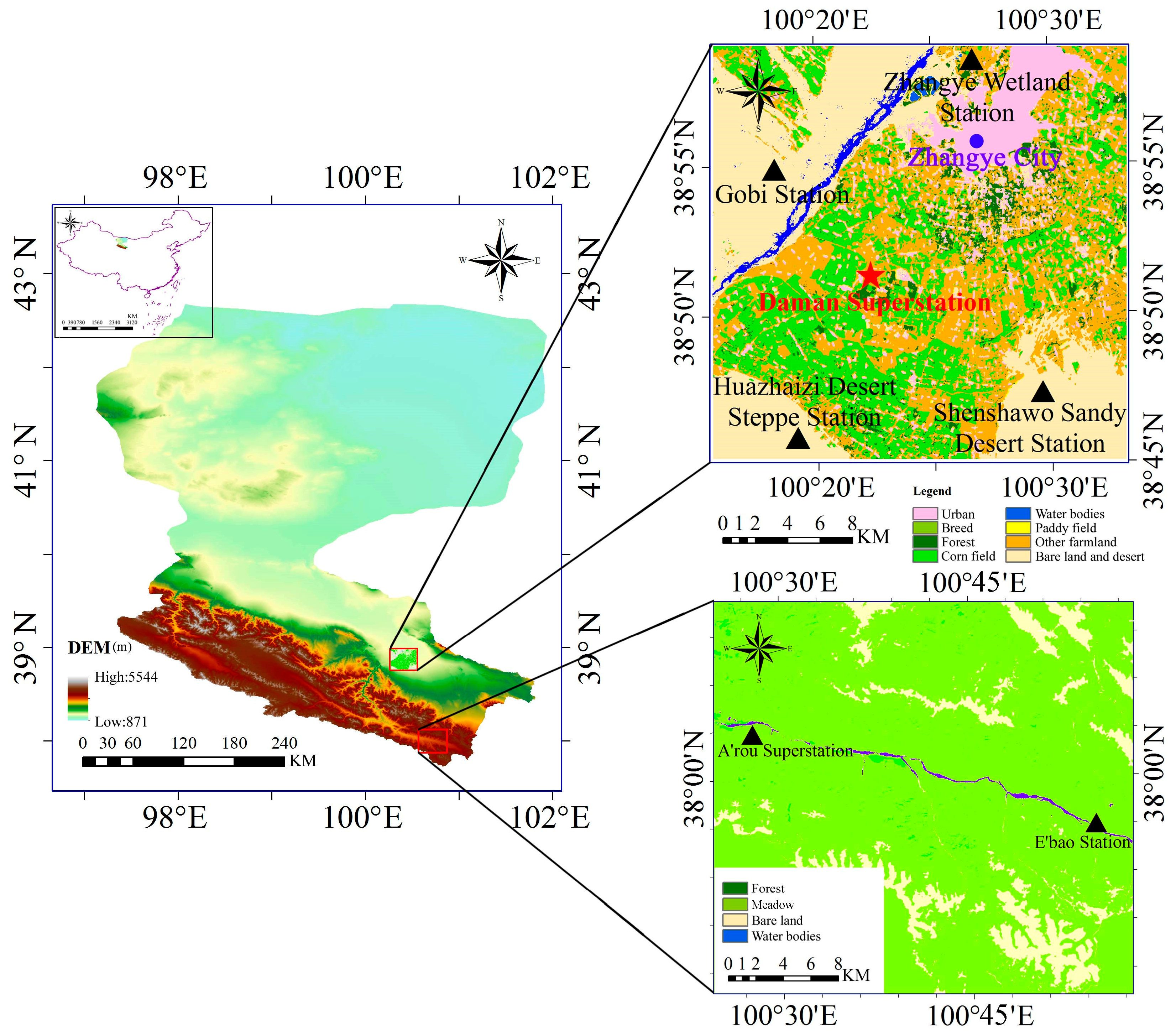
2.1. Study Area
2.2. Data
3. Methods
3.1. Auxiliary Information
3.1.1. Apparent Thermal Inertia (ATI)
3.1.2. Evaporation (E)
3.1.3. Ratio of Evaporation and Actual Evapotranspiration (E/ETa)
3.1.4. Ratio of Evaporation and Potential Evapotranspiration (E/ETp)
3.1.5. Evaporative Fraction (EF)
3.1.6. Actual Evaporative Fraction (AEF)
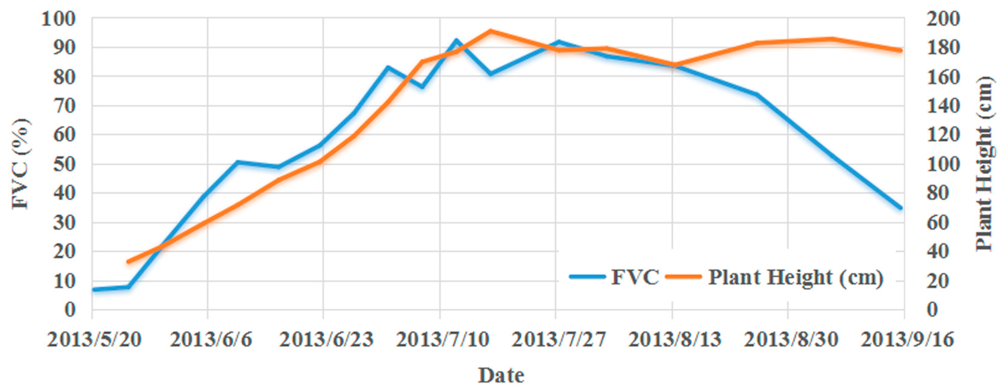
3.2. Vegetation Growth Seasons
4. Results and Discussion
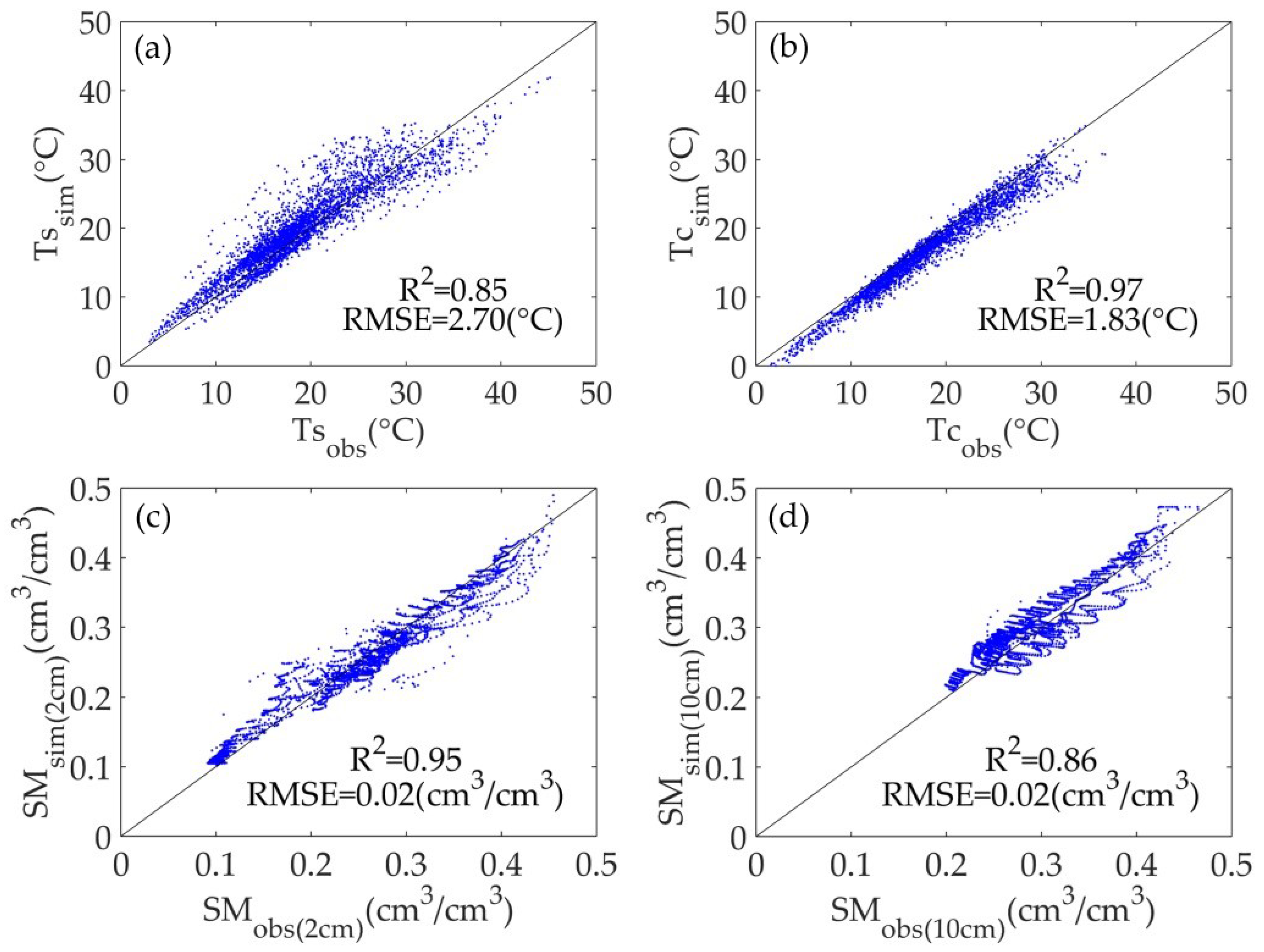
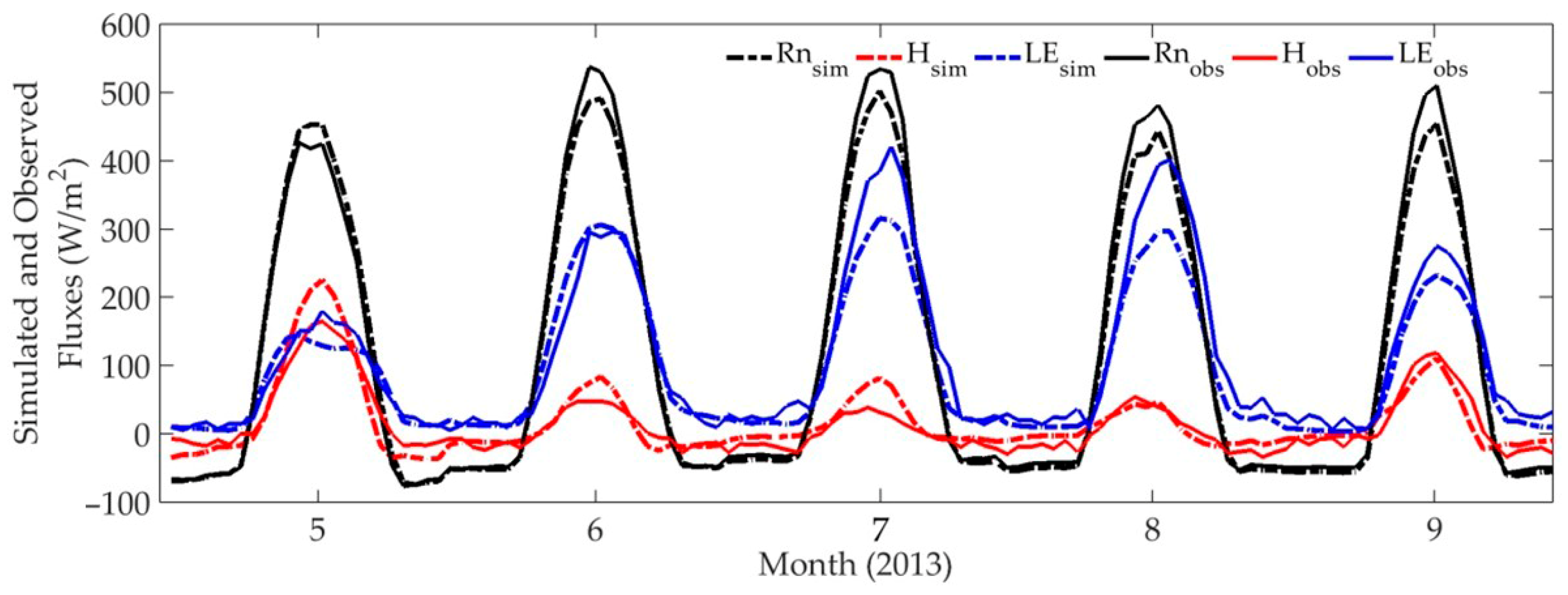
4.1. Validation of SiB2 Simulation
4.2. Correlation Analysis Between the Auxiliary Variables and Soil Moisture
4.3. Validation of Auxiliary Variables Applicability in Different Areas
4.4. Discussion
5. Conclusions
Author Contributions
Funding
Data Availability Statement
Acknowledgments
Conflicts of Interest
Appendix A

| Variables | Definition | Required Inputs | Data Source |
|---|---|---|---|
| Apparent Thermal Inertia (ATI) | A function of the difference between the LSTs in the daytime and at nighttime | Broadband albedo, daily maximum and minimum temperatures | SiB2 simulation outputs |
| Evaporation (E) | Water loss directly from the soil surface | Net radiation, ground heat flux, meteorological data | SiB2 simulation outputs |
| Actual Evapotranspiration (ETa) | Combined water loss from soil evaporation and vegetation transpiration | Energy fluxes; meteorological data | SiB2 simulation outputs |
| Potential Evapotranspiration (ETp) | Theoretical maximum evapotranspiration assuming unlimited water supply | Meteorological data; inputs for the Penman–Monteith formula | Calculated from meteorological data using the Penman–Monteith formula |
| E/ETa | The ratio of soil evaporation to actual evapotranspiration | E, ETa | SiB2 simulation outputs |
| E/ETp | The ratio of soil evaporation to potential evapotranspiration | E, ETp | SiB2 simulation outputs and the Penman–Monteith formula |
| Evaporative Fraction (EF) | The ratio of latent heat flux to the net available energy at the soil surface | Latent heat flux, net radiation, ground heat flux | SiB2 simulation outputs |
| Actual Evaporative Fraction (AEF) | The ratio of actual to potential evapotranspiration, reflecting water availability | Actual and potential evapotranspiration (ETa and ETp) | SiB2 simulation outputs and the Penman–Monteith formula |
References
- Hollmann, R.; Merchant, C.J.; Saunders, R.; Downy, C.; Buchwitz, M.; Cazenave, A.; Chuvieco, E.; Defourny, P.; de Leeuw, G.; Forsberg, R. The ESA climate change initiative: Satellite data records for essential climate variables. Bull. Am. Meteorol. Soc. 2013, 94, 1541–1552. [Google Scholar] [CrossRef]
- Ochsner, T.E.; Cosh, M.H.; Cuenca, R.H.; Dorigo, W.A.; Draper, C.S.; Hagimoto, Y.; Kerr, Y.H.; Njoku, E.G.; Small, E.E.; Zreda, M. State of the Art in Large-Scale Soil Moisture Monitoring. Soil Sci. Soc. Am. J. 2013, 77, 1888–1919. [Google Scholar]
- Wagner, W.; Bloschl, G.; Pampaloni, P.; Calvet, J.C.; Bizzarri, B.; Wigneron, J.P.; Kerr, Y. Operational readiness of microwave remote sensing of soil moisture for hydrologic applications. Water Policy 2007, 38, 1–20. [Google Scholar] [CrossRef]
- Seneviratne, S.I.; Corti, T.; Davin, E.L.; Hirschi, M.; Jaeger, E.B.; Lehner, I.; Orlowsky, B.; Teuling, A.J. Investigating soil moisture–climate interactions in a changing climate: A review. Earth-Sci. Rev. 2010, 99, 125–161. [Google Scholar] [CrossRef]
- Western, A.W.; Grayson, R.B.; Blöschl, G. Scaling of Soil Moisture: A Hydrologic Perspective. Annu. Rev. Earth Planet. Sci. 2003, 8, 149–180. [Google Scholar] [CrossRef]
- Kim, J.; Hogue, T.S. Improving Spatial Soil Moisture Representation Through Integration of AMSR-E and MODIS Products. IEEE Trans. Geosci. Remote Sens. 2012, 50, 446–460. [Google Scholar] [CrossRef]
- Vereecken, H.; Amelung, W.; Bauke, S.L.; Bogena, H.; Brüggemann, N.; Montzka, C.; Vanderborght, J.; Bechtold, M.; Blöschl, G.; Carminati, A. Soil hydrology in the Earth system. Nat. Rev. Earth Environ. 2022, 3, 573–587. [Google Scholar]
- Zhang, J.; Zhou, Z.; Yao, F.; Yang, L.; Hao, C. Validating the modified perpendicular drought index in the North China region using in situ soil moisture measurement. IEEE Geosci. Remote Sens. Lett. 2014, 12, 542–546. [Google Scholar] [CrossRef]
- Smith, K.A.; Barker, L.J.; Tanguy, M.; Parry, S.; Harrigan, S.; Legg, T.P.; Prudhomme, C.; Hannaford, J. A multi-objective ensemble approach to hydrological modelling in the UK: An application to historic drought reconstruction. Hydrol. Earth Syst. Sci. 2019, 23, 3247–3268. [Google Scholar] [CrossRef]
- Ghasemloo, N.; Matkan, A.A.; Alimohammadi, A.; Aghighi, H.; Mirbagheri, B. Estimating the agricultural farm soil moisture using spectral indices of Landsat 8, and Sentinel-1, and artificial neural networks. J. Geovisualization Spat. Anal. 2022, 6, 19. [Google Scholar] [CrossRef]
- Hunt, K.M.; Turner, A.G. The effect of soil moisture perturbations on Indian monsoon depressions in a numerical weather prediction model. J. Clim. 2017, 30, 8811–8823. [Google Scholar] [CrossRef]
- Scipal, K.; Drusch, M.; Wagner, W. Assimilation of a ERS scatterometer derived soil moisture index in the ECMWF numerical weather prediction system. Adv. Water Resour. 2008, 31, 1101–1112. [Google Scholar] [CrossRef]
- Njoku, E.G.; Chan, S.K. Vegetation and surface roughness effects on AMSR-E land observations. Remote Sens. Environ. 2006, 100, 190–199. [Google Scholar]
- Kerr, Y.H.; Waldteufel, P.; Richaume, P.; Wigneron, J.P.; Ferrazzoli, P.; Mahmoodi, A.; Bitar, A.A.; Cabot, F.; Gruhier, C.; Juglea, S.E. The SMOS Soil Moisture Retrieval Algorithm. IEEE Trans. Geosci. Remote Sens. 2012, 50, 1384–1403. [Google Scholar]
- Li, Z.-L.; Leng, P.; Zhou, C.; Chen, K.-S.; Zhou, F.-C.; Shang, G.-F. Soil moisture retrieval from remote sensing measurements: Current knowledge and directions for the future. Earth-Sci. Rev. 2021, 218, 103673. [Google Scholar]
- Kerr, Y.H.; Waldteufel, P.; Wigneron, J.P.; Martinuzzi, J.; Font, J.; Berger, M. Soil moisture retrieval from space: The Soil Moisture and Ocean Salinity (SMOS) mission. IEEE Trans. Geosci. Remote Sens. 2002, 39, 1729–1735. [Google Scholar]
- Entekhabi, D.; Njoku, E.G.; Neill, P.E.O.; Kellogg, K.H.; Crow, W.T.; Edelstein, W.N.; Entin, J.K.; Goodman, S.D.; Jackson, T.J.; Johnson, J. The Soil Moisture Active Passive (SMAP) Mission. Proc. IEEE 2010, 98, 704–716. [Google Scholar] [CrossRef]
- Chen, Y.; Yang, K.; Qin, J.; Cui, Q.; Lu, H.; Zhu, L.; Han, M.; Tang, W. Evaluation of SMAP, SMOS, and AMSR2 soil moisture retrievals against observations from two networks on the Tibetan Plateau. J. Geophys. Res. Atmos. 2017, 122, 5780–5792. [Google Scholar]
- Entekhabi, D.; Asrar, G.R.; Betts, A.K.; Beven, K.J.; Bras, R.L.; Duffy, C.J.; Dunne, T.; Koster, R.D.; Lettenmaier, D.P.; McLaughlin, D.B. An agenda for land surface hydrology research and a call for the second international hydrological decade. Bull. Am. Meteorol. Soc. 1999, 80, 2043–2058. [Google Scholar]
- Merlin, O.; Chehbouni, A.; Boulet, G.; Kerr, Y. Assimilation of disaggregated microwave soil moisture into a hydrologic model using coarse-scale meteorological data. J. Hydrometeorol. 2006, 7, 1308–1322. [Google Scholar]
- Song, C.; Hu, G.; Wang, Y.; Qu, X. Downscaling ESA CCI Soil Moisture Based on Soil and Vegetation Component Temperatures Derived From MODIS Data. IEEE J. Sel. Top. Appl. Earth Obs. Remote Sens. 2022, 15, 2175–2184. [Google Scholar]
- Peng, J.; Loew, A.; Merlin, O.; Verhoest, N.E. A review of spatial downscaling of satellite remotely sensed soil moisture. Rev. Geophys. 2017, 55, 341–366. [Google Scholar]
- Senanayake, I.P.; Pathira Arachchilage, K.R.; Yeo, I.-Y.; Khaki, M.; Han, S.-C.; Dahlhaus, P.G. Spatial downscaling of satellite-based soil moisture products using machine learning techniques: A review. Remote Sens. 2024, 16, 2067. [Google Scholar] [CrossRef]
- Liu, J.; Rahmani, F.; Lawson, K.; Shen, C. A multiscale deep learning model for soil moisture integrating satellite and in situ data. Geophys. Res. Lett. 2022, 49, e2021GL096847. [Google Scholar]
- Poehls, J.; Alonso, L.; Koirala, S.; Reichstein, M.; Carvalhais, N. Downscaling soil moisture to sub-km resolutions with simple machine learning ensembles. J. Hydrol. 2025, 652, 132624. [Google Scholar] [CrossRef]
- Qin, J.; Yang, K.; Lu, N.; Chen, Y.; Zhao, L.; Han, M. Spatial upscaling of in-situ soil moisture measurements based on MODIS-derived apparent thermal inertia. Remote Sens. Environ. 2013, 138, 1–9. [Google Scholar]
- Al Bitar, A.; Leroux, D.; Kerr, Y.H.; Merlin, O. Evaluation of SMOS Soil Moisture Products Over Continental U.S. Using the SCAN/SNOTEL Network. Geosci. Remote Sens. IEEE Trans. 2012, 50, 1572–1586. [Google Scholar]
- Jackson, T.J.; Bindlish, R.; Cosh, M.H.; Zhao, T. Validation of Soil Moisture and Ocean Salinity (SMOS) Soil Moisture Over Watershed Networks in the U.S. Geosci. Remote Sens. IEEE Trans. 2012, 50, 1530–1543. [Google Scholar]
- Sanchez, N.; Martinez-Fernandez, J.; Scaini, A.; Perez-Gutierrez, C. Validation of the SMOS L2 Soil Moisture Data in the REMEDHUS Network (Spain). IEEE Trans. Geosci. Remote Sens. 2012, 50, 1602–1611. [Google Scholar]
- Jin, R.; Li, X.; Yan, B.; Li, X.; Luo, W.; Ma, M.; Guo, J.; Kang, J.; Zhu, Z.; Zhao, S. A Nested Ecohydrological Wireless Sensor Network for Capturing the Surface Heterogeneity in the Midstream Areas of the Heihe River Basin, China. IEEE Geosci. Remote Sens. Lett. 2014, 11, 2015–2019. [Google Scholar]
- Qin, J.; Zhao, L.; Chen, Y.; Yang, K.; Yang, Y.; Chen, Z.; Lu, H. Inter-comparison of spatial upscaling methods for evaluation of satellite-based soil moisture. J. Hydrol. 2015, 523, 170–178. [Google Scholar] [CrossRef]
- Bai, X.; Wang, Z.; Wu, J.; Zhang, Z.; Zhang, P. A novel multivariate multiscale index for drought-flood abrupt alternations: Considering precipitation, evapotranspiration, and soil moisture. J. Hydrol. 2024, 643, 132039. [Google Scholar] [CrossRef]
- Carlson, T.N.; Gillies, R.R.; Perry, E.M. A Method to Make Use of Thermal Infrared Temperature and NDVI measurements to Infer Surface Soil Water Content and Fractional Vegetation Cover. Remote Sens. Rev. 1994, 9, 161–173. [Google Scholar] [CrossRef]
- Zhao, Z.; Jin, R.; Kang, J.; Ma, C.; Wang, W. Using of Remote Sensing-Based Auxiliary Variables for Soil Moisture Scaling and Mapping. Remote Sens. 2022, 14, 3373. [Google Scholar] [CrossRef]
- Price, J.C. On the analysis of thermal infrared imagery: The limited utility of apparent thermal inertia. Remote Sens. Environ. 1985, 18, 59–73. [Google Scholar] [CrossRef]
- Gao, S.; Zhu, Z.; Weng, H.; Zhang, J. Upscaling of sparse in situ soil moisture observations by integrating auxiliary information from remote sensing. Int. J. Remote Sens. 2017, 38, 4782–4803. [Google Scholar] [CrossRef]
- Knipper, K.R.; Hogue, T.S.; Franz, K.J.; Scott, R.L. Downscaling SMAP and SMOS soil moisture with moderate-resolution imaging spectroradiometer visible and infrared products over southern Arizona. J. Appl. Remote Sens. 2017, 11, 026021. [Google Scholar] [CrossRef]
- Chauhan, N.; Miller, S.; Ardanuy, P. Spaceborne soil moisture estimation at high resolution: A microwave-optical/IR synergistic approach. Int. J. Remote Sens. 2003, 24, 4599–4622. [Google Scholar] [CrossRef]
- Sánchez, N.; Gonzálezzamora, Á.; Piles, M.; Martínezfernández, J. A New Soil Moisture Agricultural Drought Index (SMADI) Integrating MODIS and SMOS Products: A Case of Study over the Iberian Peninsula. Remote Sens. 2016, 8, 287. [Google Scholar] [CrossRef]
- Amani, M.; Salehi, B.; Mahdavi, S.; Masjedi, A.; Dehnavi, S. Temperature-Vegetation-soil Moisture Dryness Index (TVMDI). Remote Sens. Environ. 2017, 197, 1–14. [Google Scholar] [CrossRef]
- Sandholt, I.; Rasmussen, K.; Andersen, J. A simple interpretation of the surface temperature/vegetation index space for assessment of surface moisture status. Remote Sens. Environ. 2002, 79, 213–224. [Google Scholar] [CrossRef]
- Kang, J.; Jin, R.; Li, X. Regression Kriging-Based Upscaling of Soil Moisture Measurements From a Wireless Sensor Network and Multiresource Remote Sensing Information Over Heterogeneous Cropland. IEEE Geosci. Remote Sens. Lett. 2015, 12, 92–96. [Google Scholar] [CrossRef]
- Kim, G.; Barros, A.P. Downscaling of remotely sensed soil moisture with a modified fractal interpolation method using contraction mapping and ancillary data. Remote Sens. Environ. 2002, 83, 400–413. [Google Scholar] [CrossRef]
- Merlin, O.; Walker, J.P.; Chehbouni, A.; Kerr, Y. Towards deterministic downscaling of SMOS soil moisture using MODIS derived soil evaporative efficiency. Remote Sens. Environ. 2008, 112, 3935–3946. [Google Scholar] [CrossRef]
- Merlin, O.; Chehbouni, A.; Walker, J.P.; Panciera, R. A Simple Method to Disaggregate Passive Microwave-Based Soil Moisture. Geosci. Remote Sens. IEEE Trans. 2008, 46, 786–796. [Google Scholar] [CrossRef]
- Gao, Q.; Zribi, M.; Escorihuela, M.; Baghdadi, N. Synergetic Use of Sentinel-1 and Sentinel-2 Data for Soil Moisture Mapping at 100 m Resolution. Sensors 2017, 17, 1966. [Google Scholar] [CrossRef]
- Bindlish, R.; Barros, A.P. Subpixel variability of remotely sensed soil moisture: An inter-comparison study of SAR and ESTAR. IEEE Trans. Geosci. Remote Sens. 2002, 40, 326–337. [Google Scholar] [CrossRef]
- Sellers, P.J. A revised land surface parameterization (SiB2) for atmospheric GCMs, Part II: The generation of global fields of terrestrial biophysical parameters from satellite data. J. Clim. 1996, 9, 706–737. [Google Scholar] [CrossRef]
- Sellers, P.J.; Randall, D.A.; Collatz, G.J.; Berry, J.A.; Field, C.B.; Dazlich, D.A.; Zhang, C.; Collelo, G.D.; Bounoua, L. A Revised Land Surface Parameterization (SiB2) for Atmospheric GCMS. Part I: Model Formulation. J. Clim. 1996, 9, 676–705. [Google Scholar] [CrossRef]
- Niu, G.Y.; Yang, Z.L.; Mitchell, K.E.; Chen, F.; Ek, M.B.; Barlage, M.; Kumar, A.; Manning, K.; Niyogi, D.; Rosero, E. The community Noah land surface model with multiparameterization options (Noah-MP): 1. Model description and evaluation with local-scale measurements. J. Geophys. Res. Atmos. 2011, 116, D12. [Google Scholar] [CrossRef]
- Dai, Y.; Zeng, X.; Dickinson, R.E.; Baker, I.; Bonan, G.B.; Bosilovich, M.G.; Denning, A.S.; Dirmeyer, P.A.; Houser, P.R.; Niu, G. The common land model. Bull. Am. Meteorol. Soc. 2003, 84, 1013–1024. [Google Scholar]
- Zhou, J.; Yang, K.; Dong, J.; Crow, W.T.; Lu, H.; Zhao, L.; Feng, H.; Tian, J.; Ma, X.; Tian, X. Mapping global soil moisture and evapotranspiration coupling strength based on a two-system method and multiple data sources. Water Resour. Res. 2025, 61, e2023WR036847. [Google Scholar] [CrossRef]
- Li, X.; Cheng, G.; Liu, S.; Xiao, Q.; Ma, M.; Jin, R.; Che, T.; Liu, Q.; Wang, W.; Qi, Y. Heihe Watershed Allied Telemetry Experimental Research (HiWATER): Scientific Objectives and Experimental Design. Bull. Am. Meteorol. Soc. 2013, 94, 1145–1160. [Google Scholar] [CrossRef]
- Li, X.; Liu, S.; Ma, M.; Xiao, Q.; Liu, Q.; Jin, R.; Che, T.; Wang, W.; Qi, Y.; Li, H. HiWATER:An Integrated Remote Sensing Experiment on Hydrological and Ecological Processes in the Heihe River Basin. Adv. Earth Sci. 2012, 27, 481–498. [Google Scholar]
- Liu, S.M.; Xu, Z.W.; Wang, W.Z.; Jia, Z.Z.; Zhu, M.J.; Bai, J.; Wang, J.M. A comparison of eddy-covariance and large aperture scintillometer measurements with respect to the energy balance closure problem. Hydrol. Earth Syst. Sci. 2011, 15, 1291–1306. [Google Scholar] [CrossRef]
- Ma, M.; Wang, X.; Wang, H.; Yu, W. HiWATER: Dataset of soil parameters in the midstream of the Heihe River Basin (2012). National Tibetan Plateau/Third Pole Environment Data Center. 2017. Available online: https://cstr.cn/18406.11.hiwater.147.2013.db (accessed on 16 February 2025). [CrossRef]
- Nishida, K.; Nemani, R.R.; Glassy, J.M.; Running, S.W. Development of an evapotranspiration index from Aqua/MODIS for monitoring surface moisture status. IEEE Trans. Geosci. Remote Sens. 2003, 41, 493–501. [Google Scholar] [CrossRef]
- Koster, R.D.; Sud, Y.; Guo, Z.; Dirmeyer, P.A.; Bonan, G.; Oleson, K.W.; Chan, E.; Verseghy, D.; Cox, P.; Davies, H. GLACE: The global land–atmosphere coupling experiment. Part I: Overview. J. Hydrometeorol. 2006, 7, 590–610. [Google Scholar]
- Shuttleworth, W.; Gurney, R.; Hsu, A.; Ormsby, J. FIFE: The variation in energy partition at surface flux sites. IAHS Publ. 1989, 186, 523–534. [Google Scholar]
- Licker, R.; Johnston, M.; Foley, J.A.; Barford, C.; Kucharik, C.J.; Monfreda, C.; Ramankutty, N. Mind the gap: How do climate and agricultural management explain the ‘yield gap’of croplands around the world? Glob. Ecol. Biogeogr. 2010, 19, 769–782. [Google Scholar]
- McVicar, T.R.; Jupp, D.L. Using covariates to spatially interpolate moisture availability in the Murray–Darling Basin: A novel use of remotely sensed data. Remote Sens. Environ. 2002, 79, 199–212. [Google Scholar]
- Van de Griend, A.; Owe, M. On the relationship between thermal emissivity and the normalized difference vegetation index for natural surfaces. Int. J. Remote Sens. 1993, 14, 1119–1131. [Google Scholar]
- Verhoef, A. Remote estimation of thermal inertia and soil heat flux for bare soil. Agric. For. Meteorol. 2004, 123, 221–236. [Google Scholar]
- Randall, D.A.; Dazlich, D.A.; Zhang, C.; Denning, A.S.; Sellers, P.J.; Tucker, C.J.; Bounoua, L.; Berry, J.A.; Collatz, G.J.; Field, C.B. A Revised Land Surface Parameterization (SiB2) for GCMS. Part III: The Greening of the Colorado State University General Circulation Model. J. Clim. 1996, 9, 738–763. [Google Scholar] [CrossRef]
- Li, Y.; Sun, R.; Liu, S. Vegetation physiological parameter setting in the Simple Biosphere model 2 (SiB2) for alpine meadows in the upper reaches of Heihe river. Sci. China Earth Sci. 2015, 58, 755–769. [Google Scholar]
- Watson, K. Regional thermal-inertia mapping from an experimental satellite. Geophysics 1982, 47, 1681–1687. [Google Scholar]
- Schlesinger, W.H.; Jasechko, S. Transpiration in the global water cycle. Agric. For. Meteorol. 2014, 189, 115–117. [Google Scholar]
- Zhao, Z.; Jin, R.; Tian, W.; Kang, J.; Su, Y. Applicability Research of Indices in Soil Moisture Downscaling based on SiB2 Simulation. Remote Sens. Technol. Appl. 2017, 32, 195–205. [Google Scholar]

| Observation Items | Instrument Installation Height (m) | Observation Instrument |
|---|---|---|
| Four components of radiation (W/m2) | 12 | PIR&PSP (Campbell) |
| Air pressure (hPa) | 2 | CS100 (Campbell) |
| Relative humidity (%) | 3, 5, 10, 15, 20, 30, 40 | AV-14TH (Avalon) |
| Horizontal wind speed (m/s) | 3, 5, 10, 15, 20, 30, 40 | Windsonic (Gill) |
| Air temperature (°C) | 3, 5, 10, 15, 20, 30, 40 | AV-14TH (Avalon) |
| Precipitation (mm) | 8, instrument height is 2.5 m | TE525MM (Texas Electronics) |
| Soil Para | Saturated Hydraulic Conductivity (mm/min) | Porosity (%) | Bulk Density (g/cm3) | Soil Texture (%) | |||
|---|---|---|---|---|---|---|---|
| Depth | Clay (<2 µm) | Silt (2–50 µm) | Sand (50–2000 µm) | ||||
| 0–5 cm | 0.300 | 0.51 | 1.312 | 5.27 | 66.01 | 28.72 | |
| 10 cm | 0.088 | 0.50 | 1.373 | 4.78 | 65.03 | 30.19 | |
| 20 cm | 0.113 | 0.49 | 1.471 | 4.46 | 67.81 | 27.73 | |
| 40 cm | 0.292 | 0.42 | 1.463 | 5.4 | 71.94 | 22.66 | |
| 60 cm | 0.135 | 0.40 | 1.530 | 5.41 | 63.57 | 31.02 | |
| 80 cm | 0.214 | 0.42 | 1.566 | 9.93 | 74.9 | 15.17 | |
| 100 cm | 0.056 | 0.41 | 1.524 | 8.48 | 73.88 | 17.64 | |
| Depth | Index | Fitting Equation at Phase I | R2 at Phase I | Fitting Equation at Phase II | R2 at Phase II |
|---|---|---|---|---|---|
| 2 cm | ATIs | ATIs = 0.0788θ0.577 | 0.45 | ATIs = 0.0822θ0.6597 | 0.59 |
| ATIc | ATIc = 0.054θ0.3839 | 0.20 | ATIc = 0.0513θ0.4054 | 0.29 | |
| E | E = 0.0997ln(θ) + 0.2184 | 0.73 | E = 0.0563ln(θ) + 0.1394 | 0.34 | |
| E/ETa | E/ETa = 19.016ln(θ) + 45.673 | 0.71 | E/ETa = 14.636ln(θ) + 36.781 | 0.56 | |
| E/ETp | E/ETp = 21.372ln(θ) + 49.243 | 0.70 | E/ETp = 16.801ln(θ) + 40.644 | 0.54 | |
| EF | EF = 48.485ln(θ) + 143.98 | 0.56 | EF = 26.175ln(θ) + 114.45 | 0.34 | |
| AEF | AEF = 60.708ln(θ) + 184.21 | 0.54 | AEF = 22.236ln(θ) + 132.85 | 0.35 | |
| 10 cm | ATIs | ATIs = 0.1155θ0.9238 | 0.50 | ATIs = 0.1213θ1.0937 | 0.51 |
| ATIc | ATIc = 0.0744θ0.6603 | 0.26 | ATIc = 0.0604θ0.609 | 0.21 | |
| E | E = 0.1443ln(θ) + 0.2616 | 0.67 | E = 0.0817ln(θ) + 0.159 | 0.22 | |
| E/ETa | E/ETa = 25.432ln(θ) + 50.876 | 0.56 | E/ETa = 23.042ln(θ) + 43.979 | 0.43 | |
| E/ETp | E/ETp = 29.805ln(θ) + 56.874 | 0.60 | E/ETp = 26.533ln(θ) + 49.004 | 0.41 | |
| EF | EF = 81.519ln(θ) + 181.72 | 0.68 | EF = 38.562ln(θ) + 124.18 | 0.23 | |
| AEF | AEF = 95.746ln(θ) + 222.25 | 0.58 | AEF = 32.407ln(θ) + 140.7 | 0.23 |
| Depth | Index | ATIs | ATIc | E | E/ETa | E/ETp | EF | AEF | |
|---|---|---|---|---|---|---|---|---|---|
| R2 | |||||||||
| 2 cm (A’rou) | R2 at Phase I | 0.43 | 0.29 | 0.41 | 0.24 | 0.53 | 0.58 | 0.68 | |
| R2 at Phase II | 0.50 | 0.31 | 0.30 | 0.51 | 0.56 | 0.28 | 0.60 | ||
| 10 cm (A’rou) | R2 at Phase I | 0.41 | 0.29 | 0.22 | 0.20 | 0.12 | 0.55 | 0.45 | |
| R2 at Phase II | 0.39 | 0.25 | 0.34 | 0.18 | 0.17 | 0.10 | 0.19 | ||
| 4 cm (E’bao) | R2 at Phase I | 0.45 | 0.23 | 0.28 | 0.18 | 0.31 | 0.22 | 0.37 | |
| R2 at Phase II | 0.31 | 0.18 | 0.30 | 0.34 | 0.33 | 0.12 | 0.26 | ||
Disclaimer/Publisher’s Note: The statements, opinions and data contained in all publications are solely those of the individual author(s) and contributor(s) and not of MDPI and/or the editor(s). MDPI and/or the editor(s) disclaim responsibility for any injury to people or property resulting from any ideas, methods, instructions or products referred to in the content. |
© 2025 by the authors. Licensee MDPI, Basel, Switzerland. This article is an open access article distributed under the terms and conditions of the Creative Commons Attribution (CC BY) license (https://creativecommons.org/licenses/by/4.0/).
Share and Cite
Zhao, Z.; Jin, R. Feasibility Research on the Auxiliary Variables in Scaling of Soil Moisture Based on the SiB2 Model: A Case Study in Daman. Electronics 2025, 14, 1392. https://doi.org/10.3390/electronics14071392
Zhao Z, Jin R. Feasibility Research on the Auxiliary Variables in Scaling of Soil Moisture Based on the SiB2 Model: A Case Study in Daman. Electronics. 2025; 14(7):1392. https://doi.org/10.3390/electronics14071392
Chicago/Turabian StyleZhao, Zebin, and Rui Jin. 2025. "Feasibility Research on the Auxiliary Variables in Scaling of Soil Moisture Based on the SiB2 Model: A Case Study in Daman" Electronics 14, no. 7: 1392. https://doi.org/10.3390/electronics14071392
APA StyleZhao, Z., & Jin, R. (2025). Feasibility Research on the Auxiliary Variables in Scaling of Soil Moisture Based on the SiB2 Model: A Case Study in Daman. Electronics, 14(7), 1392. https://doi.org/10.3390/electronics14071392