Calibration-Enhanced Multi-Awareness Network for Joint Classification of Hyperspectral and LiDAR Data

Abstract

Hyperspectral image (HSI) and light detection and ranging (LiDAR) data joint classification has been applied in the field of ground category recognition. However, existing methods still perform poorly in extracting high-dimensional features and elevation information, resulting in insufficient data classification accuracy. To address this challenge, we propose a novel and efficient Calibration-Enhanced Multi-Awareness Network (CEMA-Net), which exploits the joint spectral–spatial–elevation features in depth to realize the accurate identification of land cover categories. Specifically, we propose a novel multi-way feature retention (MFR) module that explores deep spectral–spatial–elevation semantic information in the data through multiple paths. In addition, we propose spectral–spatial-aware enhancement (SAE) and elevation-aware enhancement (EAE) modules, which effectively enhance the awareness of ground objects that are sensitive to spectral and elevation information. Furthermore, to address the significant representation disparities and spatial misalignments between multi-source features, we propose a spectral–spatial–elevation feature calibration fusion (SFCF) module to efficiently integrate complementary characteristics from heterogeneous features. It incorporates two key advantages: (1) efficient learning of discriminative features from multi-source data, and (2) adaptive calibration of spatial differences. Comparative experimental results on the MUUFL, Trento, and Augsburg datasets demonstrate that CEMA-Net outperforms existing state-of-the-art methods, achieving superior classification accuracy with better feature map precision and minimal noise.

1. Introduction

In recent years, advancements in remote sensing and imaging technologies have significantly expanded the range and detail of geomorphological data available for analysis [1,2,3,4,5]. Joint classification of hyperspectral image (HSI) and LiDAR data has become increasingly vital, with numerous studies exploring its potential [6]. Hyperspectral remote sensing provides detailed spectral information across continuous bands, often numbering in the hundreds, enabling precise surface characterization [7]. In parallel, LiDAR technology captures elevation data by using laser pulses to measure the spatial distribution of target objects on the surface [8,9]. With improved imaging and data interpretation techniques, HSI-LiDAR data fusion is playing an essential role in geological exploration [10], environmental monitoring [11], urban planning [12], and other applications.

Historically, remote sensing technology was limited in data type and accessibility, impacting the accuracy and efficiency of surface classification tasks, which depend heavily on the quality of the data source [13]. HSI data, by capturing continuous spectral variations, provides a detailed response to the material and spatial characteristics of objects [14]. However, in single-scene classifications, some objects, such as forests and agricultural areas, may exhibit similar spectral signatures, making it challenging to differentiate them based on spectral data alone, especially with HSI’s limited spatial resolution [15]. Adding LiDAR-derived elevation information to HSI data addresses this challenge by enhancing land cover classification with precise height-based distinctions [16]. Consequently, the effective integration of HSI and LiDAR data is essential for improving classification accuracy and efficiency, fostering better applications in land cover analysis and beyond.

Over recent decades, researchers have adapted various machine learning and pattern recognition models for remote sensing image classification, including support vector machines (SVM) [17], random forests (RF) [18], and extreme learning machines (ELM) [19]. These methods laid foundational advancements in image classification by leveraging spectral–spatial features effectively [20,21]. Researchers have also introduced innovative approaches to improve HSI classification. For instance, Hang et al. [22] proposed a matrix-based spectral–spatial feature representation, enhancing ground information accuracy by embedding HSI pixels into a discriminative feature subspace. Wang et al. [23] developed a multi-kernel learning framework to maximize kernel separability, which improves classification without stringent kernel restrictions. Additionally, Xing et al. [24] advanced spectral–spatial feature quality by employing low-rank learning with regularization for better feature separation. However, these methods often rely on extensive prior knowledge and complex tuning, limiting their applicability for highly non-linear and complex data scenarios [15].

More recently, Deep Neural Networks (DNNs) have significantly transformed remote sensing image analysis and classification [7,25,26]. Among these, convolutional neural networks (CNNs) are particularly notable for their ability to automatically extract deep, relevant features, enabling robust classification across diverse data types. Unlike traditional models that require manual feature extraction, CNNs and other DNNs adaptively handle complex data variations, making them suitable for various remote sensing tasks [27]. For example, Paoletti et al. [28] introduced a convolutional residual pyramid network to address the noise and redundancy issues often present in high-dimensional HSI data, providing a model with fast convergence and high accuracy. Similarly, Roy et al. [29] developed a hybrid architecture combining 3D-CNN and 2D-CNN, significantly enhancing spectral–spatial information fusion for improved classification performance. Recently, Vision Transformer (ViT)-based models have gained attention in HSI classification, pushing forward the capabilities of remote sensing models [30,31,32]. For instance, Mei et al. [33] introduced the Group-Aware Hierarchical Transformer, which enhances local and global spectral–spatial interactions through grouped pixel embeddings.

In LiDAR data classification, research primarily focuses on point cloud processing. For example, Wen et al. [34] proposed the Direction-constrained Fully Convolutional Neural Network (D-FCN), which processes raw 3D coordinates and LiDAR intensity data, offering a more efficient approach to semantic labeling of 3D point clouds. Similarly, Zorzi et al. [35] integrated CNNs and Fully Convolutional Networks (FCNs) for point cloud pixel labeling, leveraging spatial and geometric relationships for improved accuracy. Despite these advancements, single-source data classification methods remain limited in comprehensiveness, confidence, and prediction accuracy due to the unique characteristics of HSI and LiDAR data. Integrating HSI and LiDAR data, therefore, offers an important avenue to enhance classification performance by addressing these limitations.

Leveraging the powerful feature extraction and fusion capabilities of deep learning models, both CNN-based and ViT-based methods have demonstrated substantial advantages in the joint classification of HSI and LiDAR data. For instance, Hang et al. [36] proposed a coupled CNN model that not only extracts spectral–spatial features from HSI but also captures elevation information from LiDAR data. Through a parameter-sharing strategy, this model integrates these heterogeneous features, marking a shift from conventional classification approaches. Zhang et al. [37] introduced the Interleaved Perceptual Convolutional Neural Network (IP-CNN), which effectively incorporates both HSI and LiDAR constraints into the fusion of multi-source structural information, achieving notable success even with limited training data. In another study, Lu et al. [38] presented Coupled Adversarial Learning-based Classification (CALC), an adversarial framework with dual generators and a discriminator that extracts shared semantic information and modality-specific details. Zhao et al. [39] designed a two-branch architecture combining CNN and Transformer encoders in a hierarchical structure, facilitating effective joint classification of heterogeneous data. Furthermore, Sun et al. [40] proposed a multi-scale lightweight fusion network, which avoids attention mechanisms, reducing training parameters while effectively capturing depth and high-order features across scales.

Despite the significant progress of DNN-based methods in joint HSI and LiDAR classification, several challenges remain when addressing complex feature environments [41,42,43]. These challenges stem from the different imaging mechanisms of each sensor, requiring separate processing of each data type to ensure accurate representation of their specific information. Additionally, the diverse application contexts of HSI and LiDAR sensors [44] lead to variations in performance emphasis for each data type, necessitating the development of models that can adaptively address these differences while capturing both local details and global context. Moreover, the inherent variation in the features of these data types demands classification models with strong adaptive capabilities to effectively fuse and complement spectral, spatial, and elevation features, ensuring accurate scene classification.

To address these challenges, we propose a novel joint classification approach for HSI and LiDAR data called the Calibration-Enhanced Multi-Awareness Network (CEMA-Net). This method consists of two primary branches: one for processing HSI features and the other for processing LiDAR features. The key innovation in CEMA-Net is the introduction of the Multi-way Feature Retention (MFR) module, which handles HSI and LiDAR data separately to extract rich spectral–spatial and elevation features. This module is designed to adapt to the unique characteristics of each data type, effectively addressing data discretization issues. To capture semantic information at multiple scales, we also propose the Spectral–spatial Aware Enhancement (SAE) and Elevation Aware Enhancement (EAE) modules. These modules are specifically tailored to the characteristics of each data source, enabling dynamic awareness of spectral, spatial, and elevation features. Finally, to address discrepancies and misalignments between feature representations from the HSI and LiDAR branches, we introduce the Spectral–spatial–elevation Feature Calibration Fusion (SFCF) module. This module learns discriminative features from both data types, effectively bridging the gap and ensuring accurate fusion of the features from the two sources.

To summarize, the main contributions of this work are as follows:

(1)

We propose a novel joint HSI-LiDAR classification method called CEMA-Net, utilizing a hybrid two-branch CNN architecture to effectively extract 3D spectral–spatial features from HSI and 2D elevation features from LiDAR, significantly improving classification accuracy.

(2)

We introduce the Multi-way Feature Retention (MFR) module for adaptive feature extraction from HSI and LiDAR, along with the SAE and EAE modules to enhance spectral, spatial, and elevation awareness, improving feature representation.

(3)

We develop the Spectral–spatial–elevation Feature Calibration Fusion (SFCF) module to recalibrate discrepancies between HSI and LiDAR data, addressing feature differences and spatial misalignments for accurate and consistent fusion.

(4)

Our method outperforms state-of-the-art approaches, with experiments on three datasets consistently demonstrating the superior performance, effectiveness, and robustness of CEMA-Net in joint classification tasks.

The structure of this paper is organized as follows: Section 2 provides a detailed introduction to CEMA-Net, highlighting its key components and operational principles. Section 3 offers a comprehensive description of the experimental datasets, outlines the experimental setup, and presents an in-depth analysis of the classification results. Finally, Section 4 concludes the paper by summarizing the main findings and proposing potential directions for future research.

2. Methodology

Figure 1 provides a detailed visual representation of the proposed CEMA-Net, illustrating its comprehensive workflow. The framework adopts a dual-branch architecture to separately process HSI and LiDAR data. Each branch is specifically designed to address the unique characteristics of the corresponding data type, ensuring that their distinctive features are effectively captured and utilized for accurate classification.

The HSI branch focuses on extracting spectral and spatial features, utilizing modules such as the Spectral–spatial Aware Enhancement (SAE) module to enhance the network’s sensitivity to spectral variations and local spatial structures. This branch leverages convolutional layers and attention mechanisms to preserve both local and global spectral–spatial relationships. The LiDAR branch is dedicated to capturing spatial and elevation information. By incorporating the Elevation Aware Enhancement (EAE) module, this branch highlights the elevation-sensitive features that are critical for distinguishing ground objects. The two branches are integrated through the Spectral–spatial–elevation Feature Calibration Fusion (SFCF) module, which ensures effective alignment and fusion of the heterogeneous features from HSI and LiDAR data. This module not only addresses the representation disparities and spatial misalignments between the two modalities but also enhances the discriminative power of the combined features.

This refined structure allows CEMA-Net to maintain critical spectral, spatial, and elevation information throughout its processing pipeline, ultimately achieving superior classification performance compared to state-of-the-art methods.

2.1. HSI and LiDAR Data Preprocessing

For the analysis, HSI data are represented as $X_H\in {\mathbb{R}}^{m\times n\times l}$ and LiDAR data as $X_L\in {\mathbb{R}}^{m\times n}$. They include the same surface information and therefore have the same ground truth. Here, m and n correspond to the spatial dimensions, while l denotes the number of spectral bands in the HSI dataset. HSI data offer extensive spectral information, with each pixel associated with a one-hot category vector. However, the high dimensionality of spectral bands introduces significant computational challenges and can lead to redundancy, as adjacent spectral bands often carry overlapping information. To address these issues, we apply Principal Component Analysis (PCA) to reduce the dimensionality of the spectral data. PCA effectively retains the most significant spectral features by projecting the original data onto a smaller set of principal components, which not only mitigates redundancy but also enhances computational efficiency. Specifically, PCA extracts the top k principal components from the HSI data, thereby reducing the spectral band count from l to k while preserving the spatial dimensions. This results in a transformed dataset denoted as $X_H^{pca}\in {\mathbb{R}}^{m\times n\times k}$.

Subsequently, we perform patch extraction using a sliding window of size $s\times s$ on both $X_H^{pca}$ and $X_L$. This process generates 3D patches from the HSI data, denoted as $X_H^P\in {\mathbb{R}}^{s\times s\times k}$, and 2D patches from the LiDAR data, represented as $X_L^P\in {\mathbb{R}}^{s\times s}$. Each patch is identified by the label of its central pixel. For edge pixels where the window size cannot be fully accommodated, we apply a padding technique with a width of $(s-1)/2$ to ensure consistent patch sizes.

Finally, we discard any pixel blocks with a label of zero and proceed to split the remaining samples into training and testing sets for further evaluation.

2.2. Spectral–Spatial–Elevation Feature Extraction

Taking advantage of Convolutional Neural Networks (CNNs) for their exceptional capability in modeling spatial context and extracting features, CNNs are particularly adept at analyzing the spectral–spatial patterns in HSI data and efficiently retrieving elevation information from LiDAR data. To achieve this, we deploy a 3D CNN that processes high-dimensional 3D patches, capturing complex spectral and spatial features for accurate local representation. Concurrently, a 2D CNN is utilized to specifically focus on the extraction of elevation-related features from the LiDAR data.

As depicted in Figure 1, we begin with the HSI data $X_H^{pca}\in {\mathbb{R}}^{m\times n\times k}$ by applying a 3D convolution (Conv3-D) to extract meaningful spectral–spatial features. The resulting feature cube’s spatial dimensions are flattened into a 2D vector. Subsequently, a 2D convolution (Conv2-D) is applied to minimize redundancy in both the spectral and spatial information.

In contrast to the processing of HSI data, the LiDAR data $X_L\in {\mathbb{R}}^{m\times n}$ are subject to a different approach. We implement two Conv2-D layers to extract surface elevation features, using convolution kernel sizes of $16@3\times 3$ and $64@3\times 3$. To accelerate training and enhance the model’s ability to capture nonlinear relationships, we introduce layer normalization and ReLU activation functions after each convolutional layer.

2.3. Multi-Way Feature Retention Module

In HSI classification tasks, relying solely on single-scale feature extraction can lead to the omission of critical spectral and elevation details. To address this, we introduce the Multi-way Feature Retention (MFR) module, designed to thoroughly investigate the rich spectral–spatial–elevation semantic information through an advanced multi-way feature extraction framework. Additionally, we propose the Spectral–spatial Aware Enhancement (SAE) module and the Elevation Aware Enhancement (EAE) module, which aim to enhance the sensitivity of features to spectral and elevation information, distinguishing between local and global perspectives by adjusting the awareness plate size.

The key strength of the MFR module is its capability for multi-level, fine-grained feature extraction. This allows for the capture of detailed features across various scales, effectively refining the representation of spectral–spatial–elevation information. We integrate the MFR module into both the HSI and LiDAR branches of our network, further enhancing them with the SAE and EAE modules.

Specifically, the MFR module operates through three parallel pathways: local, global, and sequential convolution. For the HSI data retention structure, the features are represented as $X_H^{conv}\in {\mathbb{R}}^{h\times w\times c}$, where h and w denote the height and width, while c represents the number of spectral bands. Initially, we apply point-wise convolution to obtain $F_H^{\prime }\in {\mathbb{R}}^{h\times w\times c}$. This is then processed through both global and local pathways to yield $F_H^{global}\in {\mathbb{R}}^{h\times w\times c}$ and $F_H^{local}\in {\mathbb{R}}^{h\times w\times c}$. The SAE module is utilized here to balance and integrate global and local information. After passing through a sequential convolutional layer, we perform element-wise addition to combine the spectral–spatial features from both pathways, followed by another convolution to produce $F_H^{serial}\in {\mathbb{R}}^{h\times w\times c}$. The final output, $F_H^{out}\in {\mathbb{R}}^{h\times w\times c}$, is obtained by summing the three results.

For the retention structure of the LiDAR data, the processing flow mirrors that of the HSI data. However, the EAE module is employed to handle the global and local information specific to elevation data.

Spectral–Spatial/Elevation Aware Enhancement Module

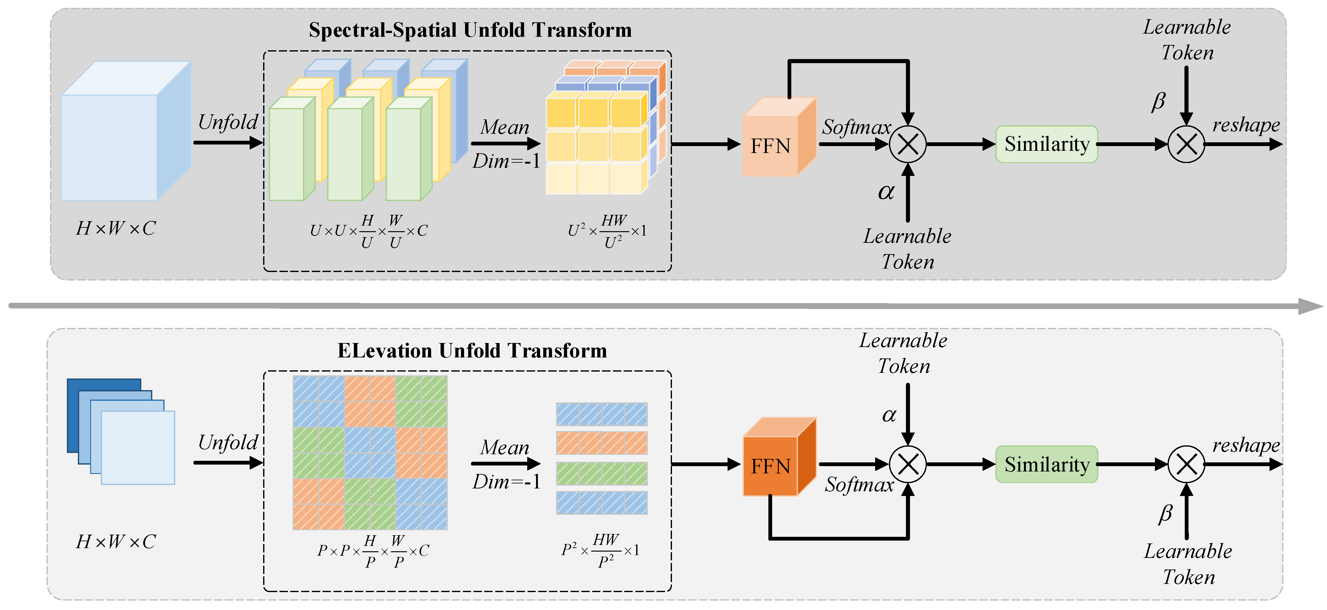
Balancing the modeling distance selection between samples is a critical challenge when dealing with large-scale, high-dimensional remote sensing images. Extracting overly localized information can distort the overall trends of spectral curves, while focusing too much on global features may overlook important texture details. To address this, we introduce the Spectral–Spatial Aware Enhancement (SAE) and Elevation Aware Enhancement (EAE) modules, which facilitate a dynamic awareness of global and local information, thereby enhancing the understanding of surface spectral changes, spatial structures, and terrain elevations.

SAE Module: As illustrated in the upper section of Figure 2, we adjust the cube parameter U to various sizes for segmenting spectral–spatial features into multiple non-overlapping blocks. Here, U can be set to $4\times 4$ for global processing or $2\times 2$ for local processing. We then employ aggregation and displacement of these non-overlapping cubes to effectively extract critical features along the spectral dimension. Additionally, we introduce a trainable parameter $\alpha$ to emphasize task-relevant tokens and perform feature selection based on the similarity matrix of the non-overlapping cubes.

Specifically, we apply an unfolding operation to flatten the spectral–spatial features into a single dimension, partitioning them into spatially adjacent, non-overlapping patches, represented as $F_H^{hsi}\in U\times U\times {\displaystyle \frac{H}{U}}\times {\displaystyle \frac{W}{U}}\times C$. To extract detailed features from these spectral–spatial data, we compress the information of each spectral band by averaging, resulting in $F_H^m\in U^2\times {\displaystyle \frac{HW}{U^2}}\times 1$. We then use a feedforward network (FFN) for linear calculations to enhance feature representation. To assess the relevance of features for remote sensing classification, we apply a sigmoid activation function to derive confidence scores in the spatial dimension, followed by element-wise multiplication to fine-tune the corresponding features.

By integrating task-specific trainable tokens into the network, we generate HSI-weighted features, defined as ${\left(f_i\right)}_{i=1}^C$, where $f_i\in {\mathbb{R}}^C$. These tokens are added to each output feature, and feature selection is performed via a similarity matrix, expressed as follows:

$$\widehat{f_i}=sim(f_i·\alpha ,f_i)·\beta$$

(1)

Here, $\alpha \in {\mathbb{R}}^{\mathbb{C}}$ represents the learnable token parameter for HSI, highlighting relevant classification features, while $\beta ={\displaystyle \frac{HW}{p^2}}$ serves as the learnable token parameter for LiDAR in the lower branch. The function $sim(·,·)$ computes cosine similarity, yielding values between 0 and 1. Each feature $f_i$ is reorganized according to its cosine similarity matrix to facilitate efficient simulated feature selection. We then execute reshaping and interpolation on each feature to produce the outputs from the global and local pathways, effectively enhancing the awareness of spectral–spatial features.

EAE Module: The awareness enhancement for elevation information, shown in the lower part of Figure 2, follows a similar processing approach as that for spectral–spatial features. Given that LiDAR elevation data are localized in the spatial dimension, we set different patch parameters P to divide it into multiple non-overlapping patches, denoted as $F_L^{patch}\in P\times P\times {\displaystyle \frac{H}{P}}\times {\displaystyle \frac{W}{P}}\times C$. Typically, P is set to 4 or 2 to represent global and local processing, respectively. We apply similar aggregation and displacement operations among the patches to extract elevation details. The similarity matrix computation for feature selection also follows this process, with a trainable parameter $\beta$ introduced as a task-specific token. The similarity matrix calculation for feature selection is given by the following:

$$\widehat{f_i}=sim(f_i·\beta ,f_i)·\alpha$$

(2)

This completes the awareness enhancement of elevation features.

2.4. Spectral–Spatial–Elevation Feature Calibration Fusion

The integration of multi-source remote sensing data is essential for improving classification performance, yet it faces significant challenges due to differences in feature representations and misalignment in spatial data. To address these issues, we introduce a novel spectral–spatial–elevation feature calibration fusion module, which effectively merges complementary features from diverse data sources, ensuring accurate and coherent integration despite inherent disparities. It incorporates two key advantages: (1) efficient learning of discriminative features from multi-source mixed data and (2) adaptive calibration of spatial differences.

Specifically, we first combine HSI and LiDAR features and dynamically learn discriminative features from the multi-source data by considering the global information importance score. To address the substantial representation differences and spatial misalignments between the multi-source features, we separately feed the features from both data types into the calibration module. There, each sub-feature is refined by applying a learnable offset, enabling more precise feature extraction. Subsequently, to achieve effective fusion of multi-source heterogeneous features, we execute element-wise multiplication between the discriminative features and the calibrated features. This facilitates enhanced information interaction and integration. Details of the spectral–spatial–elevation feature calibration module are shown in Figure 3.

A. 

Discriminative Feature Extraction:

In order to obtain unique discriminative features, we first sum the both source features according to the channel dimensions to initially obtain the joint features $F_J\in {\mathbb{R}}^{C\times H\times W}$. Following global average pooling (GAP), each channel is condensed into a feature map with spatial dimensions of $1\times 1$. Next, we introduce Sigmoid functions to normalize weights across 0 and 1. These weights are then utilized to adjust the joint feature to $F_J^{\prime }\in {\mathbb{R}}^{C\times H\times W}$, thereby amplifying information-enriched bands while diminishing the impact of irrelevant ones. This feature will be added at the end with the two enhanced features from the calibration operation to achieve the alignment of the multi-source data deviation.

B. 

Adaptive Calibration Difference:

As depicted in Figure 3, we divide the spectral–spatial and elevation features into multiple sub-features according to the dimension of the channel, and learn subtle differences in spectral–spatial and elevation information through multiple learnable offsets.

We achieve feature calibration by employing feature resampling. Specifically, given HSI features $F_H^{\prime }\in {\mathbb{R}}^{C\times H\times W}$, we first partition $F_H^{\prime }$ into G groups along the channel dimension. Spatial coordinates of pixel positions are defined as $\left[\right(1,1),(1,2),\dots \dots (H,W\left)\right]$. For each group, a learnable 2D offset ${\Delta }_{\kappa }\in {\mathbb{R}}^{2\times \times H\times W}$ is defined to learn spatial offsets. Our calibration function $\zeta (·)$ can be defined as follows:

$$\begin{array}{cc}\hfill {\mathcal{M}}_{h,w}& =\sum _{h^{\prime }}^H\sum _{w^{\prime }}^W{F}_H^{\prime }·max(0,1-|h+{\Delta }_{h,w}^1-h^{\prime })\hfill \\ \hfill & ·max(0,1-|w+{\Delta }_{h,w}^2-w^{\prime })\hfill \end{array}$$

(3)

where ${\mathcal{M}}_{h,w}$ represents the output obtained at pixel point $p=(h+{\Delta }_{h,w}^1,w+{\Delta }_{h,w}^2)$, where h and w are the height and width of the feature, respectively. ${\Delta }_{h,w}^1$ and ${\Delta }_{h,w}^2$ denote the displacement generated at the pixel point, $w^{\prime }$ and $h^{\prime }$ are the pixel positions after feature subsampling. For any position p, we enumerate all integral positions and use subsampling to obtain precise feature points at the sampling positions. Specifically, we perform subsampling on the current coordinates and obtain the most favorable features to replace the current pixel value for calibration.

$F_{\mathcal{H}}^{\prime }$ typically contains rich spectral–spatial features, while $F_{\mathcal{L}}^{\prime }$ contains more elevation features. Calibrating and merging offsets alone does not significantly enhance the performance of remote sensing classification missions. A main reason is that simple calibration and fusion cannot eliminate the feature differences of heterogeneous modes. Therefore, we further propose to selectively emphasize the calibrated complementary features through pixel masks to bridge the representational gap between them:

$$O=({\beta }_{\mathcal{H}}\otimes F_{\mathcal{H}}^{\prime }+{\beta }_{\mathcal{L}}\otimes F_{\mathcal{L}}^{\prime })\oplus F_J^{\prime }$$

(4)

where ${\beta }_{\mathcal{H}}$ and ${\beta }_{\mathcal{L}}$ denote the gate mask.

3. Experimental Setup and Discussion

We provide a detailed description of the experimental setup and results. Initially, we outline the specific datasets, experimental configurations, and evaluation metrics used to ensure a fair comparison. Next, we perform quantitative experiments on three representative multi-modal datasets to showcase the superior performance of our proposed CEMA-Net. Additionally, we conduct comprehensive ablation studies to analyze the contribution of each component within the model. Finally, both quantitative and visual results demonstrate that CEMA-Net outperforms existing state-of-the-art methods in remote sensing classification tasks.

3.1. Description of the Datasets Used

Consistent with prior studies [26,38], we selected three widely recognized datasets for remote sensing classification: MUUFL, Trento, and Augsburg. Each dataset contains both HSI and LiDAR data, as outlined in

Table 1. Training and test samples in MUUFL, Trento, and Augsburg.

Class	MUUFL			Trento			Augsburg
	Land Cover	Train	Test	Land Cover	Train	Test	Land Cover	Train	Test
01	Trees Mostly	465	22,781	Apple Trees	41	3993	Forest	271	13,236
02	Grass	86	4184	Buildings	30	2873	Residential Area	607	29,722
03	Mixed Ground Surface	138	6744	Ground	5	474	Industrial Area	78	3773
04	Dirt and Sand	37	1789	Woods	92	9031	Low Plants	538	26,319
05	Road	134	6553	Vineyard	106	10,395	Allotment	12	563
06	Water	10	456	Roads	32	3142	Commercial Area	33	1612
07	Buildings Shadow	45	2188				Water	31	1499
08	Buildings	125	6115
09	Sidewalk	28	1357
10	Yellow Curb	4	179
11	Cloth Panels	6	263
	Total	1078	52,609	Total	306	29,908	Total	1570	76,724

, which summarize the sample count and land cover categories of each.

It is worth noting that HSI and LiDAR data in these datasets were not captured simultaneously due to the inherent differences in sensor technologies and acquisition conditions. However, the datasets underwent rigorous pre-registration processes to ensure spatial alignment, allowing pixel-to-pixel correspondence between the modalities. This alignment enables the effective fusion of spectral, spatial, and elevation information from HSI and LiDAR data, which is critical for our proposed method.

(1) MUUFL Dataset: Collected at the University of Southern Mississippi’s Gulf Park campus, the MUUFL dataset combines HSI with LiDAR data, captured using a reflective optical spectrometer [45]. The HSI data span 72 spectral bands from 0.38 to 1.05 $\mathsf{\mu }$m, while the LiDAR data are represented by two rasters at a wavelength of 1.06 $\mathsf{\mu }$m. With a resolution of 325 × 220 pixels, this dataset covers 11 land cover categories. To reduce noise, the initial and final eight spectral bands, which are most affected by noise, are omitted during training. Figure 4 illustrates the dataset with pseudo-color composite images of the HSI data, grayscale LiDAR images, and land cover category maps.

(2) Trento Dataset:

The dataset covers rural areas around Trento in southern Italy and includes six distinct scenes [46]. It combines LiDAR data, collected using the Optech ALTM 3100EA sensor, with hyperspectral data from the AISA Eagle system [39]. Both sensors achieve a spatial resolution of 1 m, with images sized at $600\times 166$ pixels. The hyperspectral data contains 63 spectral bands spanning wavelengths from 402.89 nm to 989.09 nm, with spectral resolution ranging from 0.42 $\mathsf{\mu }$m to 0.99 $\mathsf{\mu }$m. The LiDAR data are represented as a single raster. Figure 5 displays the hyperspectral and LiDAR data, along with the ground truth land cover categories.

(3) Augsburg Dataset:

This dataset, collected from Augsburg, Germany, combines hyperspectral and LiDAR data for land cover analysis [47]. The hyperspectral data includes 180 spectral bands, covering wavelengths from 0.4 $\mathsf{\mu }$m (spanning UV and visible light) to 2.5 $\mathsf{\mu }$m (extending into the near-infrared). The LiDAR data, captured at a wavelength of 1.06 $\mathsf{\mu }$m, is represented as a single raster layer. Both data types have a spatial resolution of 30 m, with each image measuring $332\times 485$ pixels. Figure 6 shows visual representations of the data, which categorize seven types of land cover.

3.2. Experimental Configuration

(1) Evaluation Metrics:

We use four standard metrics to assess the performance of our proposed CEMA-Net: overall accuracy (OA), average accuracy (AA), kappa coefficient (k), and per-class accuracy. These metrics serve as indicators of classification accuracy, and our objective is to achieve the highest possible values in each. Specifically, overall accuracy (OA) is the ratio of correctly classified pixels to the total number of pixels in the dataset. Average accuracy (AA) is the mean value of the classification accuracies for each individual class. Kappa coefficient (k) measures the agreement between the predicted and actual class labels, accounting for the possibility of agreement occurring by chance. Per-class accuracy evaluates the classification performance for each individual class, providing a detailed measure of how well each class is recognized. To ensure a fair and consistent comparison, all experiments are carried out with separate training and testing datasets.

(2) Environment Configuration:

Our CEMA-Net model is implemented in PyTorch 2.2.0, utilizing the Adam optimizer with parameters ${\beta }_1=0.9$ and ${\beta }_2=0.999$. The training process spans 100 epochs, with a batch size of 64 and an initial learning rate set to $1\times {10}^{-3}$. It is executed on an NVIDIA Geforce RTX 4090 GPU with 24 GB of VRAM. In contrast, traditional methods for comparison are run on the MATLAB platform (https://matlab.zszlxx.cn/index.html?bd_vid=8287305137028280579, accessed on 9 November 2024).

3.3. Hyperparameter Configuration

(1) Patch Size: In the joint classification of HSI and LiDAR data, selecting the optimal patch size is crucial for balancing the ability to capture spatial distribution, spectral variations, and elevation information while keeping computational costs manageable. In the previous experiments, all parameters were fixed except for the patch size. To identify the best patch size, we evaluated the accuracy of several patch sizes from the set 7, 9, 11, 13, 15, 17. As illustrated in Figure 7, excessively large patch sizes result in more complex inputs, particularly impacting the scalar fusion module and diminishing the network’s fitting capacity, thus reducing accuracy. On the other hand, too small a patch size leads to a lack of sufficient contextual information, impairing global feature retention and accuracy. Based on these results, a patch size of 11 was found to be optimal for the classification task.

(2) Reduced Spectral Dimension: HSI offers extensive spectral information with hundreds of continuous bands, which can capture detailed features of ground objects. However, the broad spectral range and high sensitivity often result in a significant amount of redundant data, contributing to the problem of “dimensionality curse”. To address this challenge, we apply Principal Component Analysis (PCA) to extract the most critical spectral components, ensuring an optimal trade-off between spectral richness and computational efficiency. As illustrated in Figure 8, retaining too few spectral bands leads to a substantial loss of important information, while a larger number of bands introduces unnecessary redundancy and increases computational costs, thus reducing classification accuracy. In our experiments, we assessed different numbers of retained spectral bands from the set 5, 10, 15, 20, 25, 30, 35, 40. The results show that selecting 30 bands strikes the best balance, significantly enhancing the integration of HSI and LiDAR data and improving classification performance.

(3) Learning Rate: The learning rate is a crucial hyperparameter that governs the size of weight updates during model training, directly impacting the speed and stability of the learning process. A high learning rate can cause instability, leading to oscillations that prevent the model from converging effectively. Conversely, a low learning rate results in slower convergence, increasing both training time and computational cost. In hyperspectral image classification tasks, choosing an optimal learning rate is essential for maintaining training stability and enhancing final classification performance. We tested various learning rates from the set {$1\times {10}^{-5}$, $5\times {10}^{-5}$, $1\times {10}^{-4}$, $5\times {10}^{-4}$, $1\times {10}^{-3}$, $5\times {10}^{-3}$} to evaluate their impact on accuracy. As shown in Figure 9, the experiments reveal that a learning rate of $5\times {10}^{-4}$ works best for the MUUFL and Augsburg datasets, while a learning rate of $1\times {10}^{-3}$ yields the most accurate results for the Trento dataset.

3.4. Ablation Experiments

Based on the results of the ablation experiments in

Table 2. Results of ablation experiments. ✓ indicates selected, × indicates unselected. Bold indicate optimal performance.

Cases	Component				Indicators
	MFR	SAE	EAE	SFCF	OA (%)	AA (%)	$\mathbf{k}\mathbf{\ast }\mathbf{100}$
1	×	✓	✓	✓	89.67	80.87	86.65
2	✓	×	✓	✓	90.27	80.95	87.05
3	✓	✓	×	✓	90.41	81.01	87.17
4	✓	✓	✓	×	90.1	80.24	86.45
5	✓	✓	✓	✓	90.88	81.56	87.98

, we evaluate the effectiveness of each component within CEMA-Net, focusing on the MFR, SAE, EAE, and SFCF modules.

Case 1: When the MFR module is removed, the model’s OA, AA, and kappa scores decrease to 89.67%, 80.87%, and 86.65, respectively. This shows that the MFR module contributes significantly to the model’s feature extraction capabilities since its absence reduces classification accuracy across all metrics.

Case 2 and Case 3: These cases exclude the SAE and EAE modules, respectively. Without the SAE module (Case 2), the OA, AA, and kappa scores are 90.27%, 80.95%, and 87.05. Without the EAE module (Case 3), the scores slightly improve to 90.41%, 81.01%, and 87.17. This suggests that while each module independently enhances classification performance, both modules work together to better capture complex spectral–spatial–elevation information since removing either leads to reduced accuracy.

Case 4: In this configuration, the SFCF module is removed, and spectral–spatial and elevation features are directly added to the classifier. This causes the OA, AA, and kappa values to fall to 90.1%, 80.24%, and 86.45, respectively, indicating that the SFCF module is essential for effective feature fusion, mitigating spatial misalignments between HSI and LiDAR data.

Case 5: With all components included, CEMA-Net achieves its best performance, with OA, AA, and Kappa scores reaching 90.88%, 81.56%, and 87.98. This underscores the importance of each module in contributing to the overall classification accuracy, with the full model demonstrating optimal performance across all metrics.

3.5. Classification Result and Analysis

To highlight the effectiveness of our proposed CEMA-Net over other state-of-the-art methods, we selected several well-regarded classification techniques, organized into two categories. The first includes HSI-based classification methods: RF [20], SVM [21], 2D-CNN [48], HybridSN [29], and GAHT [33]. The second category comprises joint HSI and LiDAR fusion methods: CoupledCNN [36], CALC [38], HCTnet [39], and M2FNet [40]. For a fair comparison, we used each method’s default parameters as specified in the respective references, applied the same training set splits, and kept other parameters consistent with our setup. Each experiment was repeated ten times to ensure robustness, and both the mean and variance of the results were calculated to provide a comprehensive evaluation of the model’s performance and stability.

(1) 

Performance Evaluation and Analysis

Table 3. Classification accuracy of MUUFL using different methods. Bold and highlighted in red indicate optimal performance.

No.	Only HSI Input					HSI and LiDAR Input
	RF [20]	SVM [21]	2D-CNN [48]	HybridSN [29]	GAHT [33]	CoupledCNN [36]	CALC [38]	HCTnet [39]	M2FNet [40]	Ours
1	95.86 ± 0.63	94.67 ± 1.13	96.88 ± 0.55	94.42 ± 1.56	95.13 ± 1.21	95.85 ± 0.31	96.87 ± 0.4	96.78 ± 0.31	96.74 ± 0.33	96.08 ± 0.6
2	76.33 ± 4.12	82.76 ± 3.68	79.11 ± 1.26	80.39 ± 1.63	73.98 ± 3.75	78.73 ± 1.09	81.07 ± 2.06	82.19 ± 2.1	81.49 ± 1.0	80.6 ± 3.88
3	80.68 ± 7.11	85.03 ± 2.08	82.05 ± 2.37	79.59 ± 2.56	81.6 ± 2.25	86.57 ± 2.48	83.84 ± 0.88	85.95 ± 0.55	84.34 ± 2.55	87.44 ± 1.49
4	86.73 ± 3.59	90.54 ± 3.41	85.29 ± 4.67	88.64 ± 1.42	80.28 ± 4.69	88.34 ± 3.44	89.49 ± 2.39	88.06 ± 2.65	89.03 ± 2.21	95.4 ± 1.68
5	86.45 ± 1.4	88.85 ± 1.13	86.41 ± 1.14	86.56 ± 0.89	85.71 ± 3.72	92.5 ± 0.75	92.79 ± 0.43	92.5 ± 0.98	88.71 ± 4.38	88.92 ± 0.59
6	90.99 ± 0.37	91.76 ± 3.77	84.97 ± 4.63	72.57 ± 24.62	63.68 ± 3.65	86.36 ± 3.06	90.79 ± 3.34	94.34 ± 2.8	96.71 ± 2.32	98.64 ± 1.42
7	75.41 ± 1.32	79.88 ± 7.8	74.5 ± 4.88	81.62 ± 2.54	61.5 ± 9.08	78.03 ± 3.21	76.32 ± 2.32	76.35 ± 1.51	80.97 ± 6.06	87.92 ± 3.07
8	95.06 ± 0.81	94.04 ± 0.23	94.99 ± 0.66	93.11 ± 1.18	92.6 ± 1.62	96.07 ± 0.28	97.7 ± 0.51	96.58 ± 0.51	96.29 ± 1.82	96.15 ± 0.35
9	29.64 ± 10.4	33.33 ± 6.06	39.11 ± 0.98	34.71 ± 4.16	21.4 ± 7.29	33.93 ± 4.08	32.07 ± 3.86	46.96 ± 2.19	46.28 ± 5.93	41.88 ± 4.49
10	1.11 ± 0.45	4.28 ± 1.15	13.22 ± 4.31	16.76 ± 6.17	10.99 ± 4.11	4.92 ± 2.77	2.35 ± 1.47	13.52 ± 1.85	21.45 ± 5.13	30.77 ± 3.17
11	40.75 ± 1.11	61.74 ± 12.17	69.95 ± 7.28	84.97 ± 4.96	53.41 ± 6.21	61.29 ± 3.86	73.31 ± 3.69	68.97 ± 3.45	74.14 ± 12.54	93.41 ± 1.13
OA(%)	87.59 ± 0.63	88.85 ± 0.38	88.71 ± 0.27	87.50 ± 0.90	85.67 ± 0.04	89.75 ± 0.58	90.26 ± 0.31	90.80 ± 0.24	90.30 ± 0.84	90.88 ± 0.29
AA(%)	69.00 ± 1.23	73.35 ± 0.39	73.32 ± 0.52	73.94 ± 1.94	65.48 ± 1.29	72.96 ± 1.52	74.24 ± 0.81	76.56 ± 0.64	77.83 ± 1.03	81.56 ± 0.67
k × 100	83.51 ± 0.80	85.29 ± 0.48	84.97 ± 0.36	83.55 ± 1.10	80.90 ± 0.09	86.43 ± 0.78	87.08 ± 0.39	87.80 ± 0.32	87.13 ± 1.14	87.98 ± 0.40

,

Table 4. Classification accuracy of Trento using different methods. Bold and highlighted in red indicate optimal performance.

No.	Only HSI Input					HSI and LiDAR Input
	RF [20]	SVM [21]	2D-CNN [48]	HybridSN [29]	GAHT [33]	CoupledCNN [36]	CALC [38]	HCTnet [39]	M2FNet [40]	Ours
1	98.59 ± 0.4	98.67 ± 0.65	99.32 ± 0.41	96.09 ± 2.85	98.74 ± 0.59	99.85 ± 0.08	99.67 ± 0.15	99.32 ± 0.21	99.46 ± 0.52	98.97 ± 0.53
2	94.15 ± 1.58	96.62 ± 0.29	93.91 ± 2.7	85.59 ± 0.34	88.82 ± 6.34	99.22 ± 0.3	98.97 ± 0.73	94.87 ± 0.7	97.42 ± 1.32	98.26 ± 0.25
3	60.69 ± 7.75	60.54 ± 21.21	66.46 ± 4.06	52.95 ± 19.39	34.74 ± 6.76	59.32 ± 10.57	71.98 ± 11.39	90.97 ± 3.37	80.89 ± 4.5	96.12 ± 1.38
4	100.0 ± 0.0	100.0 ± 0.0	99.97 ± 0.04	99.88 ± 0.12	99.64 ± 0.48	100.0 ± 0.0	99.97 ± 0.02	99.97 ± 0.03	100.0 ± 0.0	100.0 ± 0.0
5	99.97 ± 0.02	99.98 ± 0.03	98.65 ± 0.96	97.87 ± 0.89	91.29 ± 12.32	99.98 ± 0.02	99.97 ± 0.01	99.9 ± 0.07	99.93 ± 0.04	100.0 ± 0.0
6	90.67 ± 0.44	90.53 ± 0.76	83.57 ± 2.18	86.24 ± 2.12	95.59 ± 0.73	97.13 ± 0.43	94.55 ± 0.88	95.98 ± 1.17	97.26 ± 0.15	97.91 ± 0.36
OA(%)	97.64 ± 0.28	97.87 ± 0.21	96.59 ± 0.67	95.13 ± 0.34	94.12 ± 5.07	98.95 ± 0.15	98.82 ± 0.21	98.81 ± 0.19	99.07 ± 0.12	99.41 ± 0.06
AA(%)	90.68 ± 1.51	91.06 ± 3.35	90.31 ± 0.43	86.44 ± 3.29	84.80 ± 4.19	92.58 ± 1.74	94.19 ± 1.90	96.84 ± 0.72	95.83 ± 0.73	98.54 ± 0.22
k × 100	96.84 ± 0.38	97.15 ± 0.28	95.45 ± 0.90	93.48 ± 0.46	92.31 ± 6.55	98.60 ± 0.20	98.43 ± 0.28	98.41 ± 0.25	98.75 ± 0.16	99.22 ± 0.08

and

Table 5. Classification accuracy of Augsburg using different methods. Bold and highlighted in red indicate optimal performance.

No.	Only HSI Input					HSI and LiDAR Input
	RF [20]	SVM [21]	2D-CNN [48]	HybridSN [29]	GAHT [33]	CoupledCNN [36]	CALC [38]	HCTnet [39]	M2FNet [40]	Ours
1	98.47 ± 0.14	96.73 ± 2.02	98.28 ± 0.23	98.17 ± 0.37	97.57 ± 0.61	97.12 ± 0.82	98.19 ± 0.16	98.96 ± 0.33	98.66 ± 0.45	99.08 ± 0.18
2	98.19 ± 0.19	98.33 ± 0.08	97.7 ± 0.18	97.0 ± 0.27	97.66 ± 0.8	97.85 ± 0.74	98.55 ± 0.18	97.8 ± 0.11	96.95 ± 1.51	97.49 ± 0.26
3	76.85 ± 3.58	76.54 ± 1.98	79.26 ± 2.23	71.72 ± 2.82	75.78 ± 8.07	82.67 ± 3.35	85.08 ± 1.97	76.24 ± 2.6	77.97 ± 9.27	84.21 ± 0.72
4	98.65 ± 0.27	98.82 ± 0.15	98.67 ± 0.07	98.76 ± 0.05	95.49 ± 1.33	98.53 ± 0.27	98.7 ± 0.07	98.61 ± 0.21	98.69 ± 0.3	98.1 ± 0.25
5	21.46 ± 5.78	20.63 ± 6.41	63.0 ± 3.11	61.41 ± 2.97	48.52 ± 15.67	76.13 ± 8.56	72.47 ± 3.63	60.81 ± 11.07	82.74 ± 4.53	92.27 ± 1.19
6	19.42 ± 8.6	19.7 ± 2.54	32.71 ± 5.95	39.44 ± 2.77	59.74 ± 6.35	51.81 ± 3.87	37.08 ± 4.98	35.15 ± 3.9	45.38 ± 16.65	60.4 ± 4.22
7	50.98 ± 2.06	50.13 ± 9.15	60.09 ± 2.05	62.86 ± 1.8	44.47 ± 1.4	58.81 ± 3.39	61.53 ± 2.12	55.66 ± 0.85	66.14 ± 1.62	66.76 ± 3.11
OA(%)	94.21 ± 0.16	93.98 ± 0.59	94.87 ± 0.08	94.42 ± 0.13	93.63 ± 0.59	95.32 ± 0.26	95.67 ± 0.09	94.80 ± 0.26	95.12 ± 0.51	95.91 ± 0.09
AA(%)	66.29 ± 1.67	65.84 ± 2.33	75.67 ± 0.51	75.62 ± 1.09	74.18 ± 3.20	80.42 ± 1.39	78.80 ± 0.61	74.75 ± 2.13	80.93 ± 1.61	85.47 ± 1.23
k×100	91.63 ± 0.25	91.30 ± 0.86	92.63 ± 0.11	92.01 ± 0.20	90.86 ± 0.83	93.28 ± 0.39	93.78 ± 0.12	92.52 ± 0.37	93.01 ± 0.70	94.15 ± 0.13

provide a quantitative comparison of CEMA-Net against various state-of-the-art methods across three datasets. Each experiment was repeated 10 times to ensure reliability, with averages and standard deviations calculated for fair comparison. In each case, the best-performing results are emphasized in bold red. Our method consistently achieves top scores in overall accuracy (OA), average accuracy (AA), and the kappa coefficient on all datasets.

Table 3 presents detailed results of each method alongside CEMA-Net on the MUUFL dataset. Across all metrics, our CEMA-Net outperforms other approaches. Unlike traditional models like RF and SVM, deep learning methods capture a wider range of features, significantly improving classification accuracy. While models such as 2D-CNN, HybridSN, and GAHT are effective at feature extraction from HSI data, their OA results are lower than those for our CEMA-Net, likely due to limited receptive fields that miss global features. Furthermore, our CEMA-Net excels in joint HSI and LiDAR data classification, showing competitive performance in metrics like OA, AA, and kappa, and demonstrating strong average accuracy across classes. It surpasses methods like CoupledCNN, CALC, HCTnet, and M2FNet in AA, largely due to the multiple receptive fields in the local-global branch and the efficient fusion strategy for spectral-elevation feature alignment.

The Trento dataset, characterized by a limited number of categories and an uneven sample distribution, results in high overall accuracy (OA) and kappa scores across all methods, yet leaves substantial room for improvement in average accuracy (AA). Table 4 shows that joint classification approaches combining HSI and LiDAR data perform well, with methods like HCTnet and M2FNet achieving solid results. HCTnet’s dual Transformer encoder effectively integrates the unique features of these two remote sensing data types; however, its complex fusion process may lead to underfitting, particularly given Trento’s limited sample size. Our proposed CEMA-Net addresses this challenge effectively. The model’s MFR module is tailored to preserve detailed data, even with fewer samples, enabling our method to surpass HCTnet in both OA and kappa. Similarly, while M2FNet leverages multi-scale feature extraction to capture spectral–spatial–elevation information, our CEMA-Net’s SAE and EAE modules, which strengthen global–local feature awareness, provide a decisive edge, outperforming M2FNet in OA, AA, and kappa metrics.

The Augsburg dataset presents distinct challenges, with its high spatial resolution and complex object information, requiring models to balance local and global information effectively. The integration of LiDAR data further enhances the value of joint classification methods over single-source approaches. As Table 5 indicates, CALC’s use of dual adversarial networks for adversarial training in the object space yields high OA, benefiting from an adversarial strategy that merges spatial and elevation data efficiently. Nonetheless, our CEMA-Net’s SFCF module enhances spatial–elevation coupling by introducing additional offsets, leading to superior data fusion. This refinement allows our CEMA-Net to outperform CALC in key metrics such as OA, AA, and kappa, while the offset correction further improves fusion stability. Across all three datasets, our extensive comparisons emphasize that our CEMA-Net marks a significant improvement in joint classification, consistently achieving top results across metrics.

(2) 

Visual Assessment and Analysis

To further highlight the generalizability of our model under different conditions, we evaluated its performance across the MUUFL, Trento, and Augsburg datasets, which differ in environmental conditions, imaging methods, and spectral characteristics. On all datasets, our model demonstrated superior performance compared to others. For example, on the Trento dataset, which includes complex landscapes, CEMA-Net was able to differentiate between small and large objects with much greater clarity, while traditional methods showed blurred boundaries. On the Augsburg dataset, where the terrain features are more varied and the spectral data are more challenging, our method still maintained high classification accuracy, further proving its robustness under varying conditions.

The comparison across these datasets demonstrates the versatility of CEMA-Net, as it consistently produces high-quality results regardless of environmental or data acquisition challenges. Our model shows excellent performance in handling diverse conditions, showcasing its effectiveness in real-world applications where datasets may vary in scale, spectral information, and terrain complexity.

Figure 10, Figure 11 and Figure 12 illustrate the visualization results for various methods, enabling a qualitative comparison of their classification performance. The differences in classification accuracy between the methods are clearly visible. Notably, our proposed CEMA-Net produces cleaner, more accurate feature maps with minimal noise.

In detail, classification methods relying solely on HSI data tend to produce results with indistinct boundaries and substantial noise. While joint classification methods using multi-source data mitigate these issues to some extent, they still underperform in accurately classifying certain ground regions. In contrast, our approach yields results with sharp boundaries and high classification accuracy. For instance, Figure 10 displays the visualization results on the MUUFL dataset, highlighting that most methods struggle with blurriness and noise, especially in differentiating densely packed small areas across multiple classes. The classification map generated by our CEMA-Net, however, aligns more closely with the actual ground truth.

Figure 11 presents the visualization results of the comparison methods on the Trento dataset. This dataset, with larger ground objects and fewer categories compared to the MUUFL dataset, is relatively easier to classify. However, we can still observe that most of the comparison methods introduce significant noise, while our method consistently achieves high-precision classification. Additionally, Figure 12 shows the classification results on the Augsburg dataset, which has a higher resolution and more complex scenes. Even in these denser areas with more categories, our CEMA-Net continues to deliver superior classification performance, demonstrating its robustness across diverse datasets.

3.6. Exploration of Results for Various Data Modalities

The results of the ablation experiments for various data modalities are shown in

Table 6. Results of ablation experiments for various data modalities. Bold indicate optimal performance.

Cases	MUUFL			Trento			Augsburg
	OA (%)	AA (%)	$\mathbf{k}\mathbf{\times }\mathbf{100}$	OA (%)	AA (%)	$\mathbf{k}\mathbf{\times }\mathbf{100}$	OA (%)	AA (%)	$\mathbf{k}\mathbf{\times }\mathbf{100}$
Only HSI	86.53	71.65	81.33	94.53	92.28	93.56	92.86	77.41	88.39
Only LiDAR	69.26	57.82	66.42	73.25	71.73	73.32	65.82	57.62	62.42
HSI + LiDAR	90.88	81.56	87.98	99.41	98.54	99.22	95.91	85.47	94.15

, which evaluates the performance of the proposed method under different data configurations on three datasets: MUUFL, Trento, and Augsburg.

Only HSI: When using only HSI data, the classification performance varied across the datasets. The OA for MUUFL was 86.53%, for Trento it was 94.53%, and for Augsburg it was 92.86%. The AA and kappa coefficient (k) were also reported, with the highest AA of 92.28% for Trento. Although HSI data provide rich spectral information, it may not fully capture the spatial and elevation features needed for accurate classification, leading to lower performance in some cases.

Only LiDAR: When using only LiDAR data, the performance dropped significantly, with the OA of 69.26% for MUUFL, 73.25% for Trento, and 65.82% for Augsburg. LiDAR data alone lack the spectral information provided by HSI, and as a result, their ability to accurately classify land cover types is limited, especially in complex or similar terrain.

HSI + LiDAR: The combination of HSI and LiDAR data yielded the best performance across all datasets. For MUUFL, the OA reached 90.88%, for Trento it was 99.41%, and for Augsburg it was 95.91%. In terms of AA and the kappa coefficient, the joint modality significantly outperformed the individual modalities, achieving the highest AA (98.54% for Trento) and kappa score (99.22 for Trento). This demonstrates the complementary nature of HSI and LiDAR data, where the fusion of spectral, spatial, and elevation features allows for more precise land cover classification.

These results highlight the importance of integrating multi-modal data, especially when leveraging both HSI and LiDAR data to enhance classification accuracy in remote sensing applications. The proposed method shows clear improvements over using individual data types, confirming the effectiveness of joint spectral–spatial–elevation feature fusion.

3.7. Model Complexity Analysis

To validate the effectiveness of the proposed model, we conducted computational complexity experiments on the MUUFL dataset, as shown in

Table 7. Compute complexity results on several models on the MUUFL dataset.

Metrics	CoupledCNN	CALC	HTCnet	M2FNet	Ours
Parameters (M)	1.98	1.75	1.85	1.67	1.34
Flops (G)	0.98	1.56	1.37	1.21	1.34
Testing Time (s)	0.76	1.15	1.37	1.05	0.92
OA (%)	89.75	90.26	90.80	90.30	90.88

. Compared to other state-of-the-art models, our method demonstrates the smallest parameter count (1.34 M), indicating a lightweight network architecture. Although the computational cost (1.34 G FLOPs) is comparable to some methods, the testing time of our model is only 0.92 s, making it the most efficient. Additionally, our model achieves the highest overall accuracy (OA) of 90.88%, slightly outperforming HTCnet (90.80%) and CALC (90.26%). These results highlight that the proposed method achieves a good balance between computational efficiency and classification performance, making it well-suited for resource-constrained scenarios, such as vehicle-based remote sensing or large-scale, real-time applications.

4. Conclusions

This paper presents CEMA-Net, a novel and highly efficient Calibration-Enhanced Multi-Awareness Network, aimed at achieving the effective fusion of spectral–spatial and elevation features to substantially boost accuracy in remote sensing classification tasks. At the core of our approach is the Multi-way Feature Retention (MFR) module, which leverages a multi-branch design to capture deep semantic information across spectral, spatial, and elevation domains, facilitating the comprehensive integration of global and local characteristics. Additionally, we introduce the Spectral–spatial Aware Enhancement (SAE) and Elevation Aware Enhancement (EAE) modules to emphasize features of ground objects that are especially responsive to spectral and elevation cues. To overcome representation discrepancies and spatial misalignments between multi-source features, we propose the Spectral–spatial–elevation Feature Calibration Fusion (SFCF) module, which effectively learns distinctive features from heterogeneous data and adaptively aligns spatial differences. Comprehensive experiments validate the advancement and resilience of our proposed method. As a future direction, we aim to adapt CEMA-Net for real-time remote sensing applications, such as autonomous vehicle navigation and drone-based land cover monitoring, where the timely and accurate classification of large-scale datasets is essential.