Analysis of Maritime Wireless Communication Connectivity Based on CNN-BiLSTM-AM

Abstract

The marine environment’s complexity poses considerable difficulties for the stability and reliability of communication links. The restricted coverage of onshore base stations in marine areas makes relay technology a critical solution for extending the communication coverage. Here, connectivity analyses help nodes select the optimal forwarding links, reducing transmission failures and improving the network performance. However, the rapid changes in marine wireless channels and the complexity of hydrological conditions make it challenging to acquire precise channel state information (CSI). In particular, dynamic environmental factors like tides, waves, and wind speed lead to substantial variations in the channel parameters over time. In response to these challenges, this paper puts forward a ship-to-shore communication system using relay ships to extend the coverage of terrestrial base stations. A novel channel modeling method is designed to capture the characteristics of marine wireless channels accurately. Additionally, a machine learning (ML)-based approach is introduced to predict the dual-hop link connection probability at future time points by analyzing historical time-series data on oceanic environmental and ship movement parameters. The proposed model consists of a convolutional-layer-based feature extractor and a bidirectional long short-term memory (BiLSTM) estimator. The CNN module extracts effective high-level features from the input data, while the BiLSTM module further explores the dependencies and dynamic patterns along the temporal dimension. The attention mechanism is introduced to distinguish the importance of the information through a weighted approach. The experimental results show that compared to traditional methods and other deep learning approaches, the proposed CNN-BiLSTM-AM model performs better in terms of its prediction accuracy and fitting ability. The model’s mean squared error (MSE) is as low as 0.0126.

1. Introduction

1.1. Background

Over the past two decades, significant advancements have been made in terrestrial wireless communication, supporting a range of high-speed, low-latency applications. In recent years, the rapid increase in maritime activities, such as oil exploration, ocean aquaculture, scientific expeditions, and tourism, has driven greater attention to providing broadband communication services for naval users.

Currently, the main approach to achieving maritime broadband communication is through accessing terrestrial base stations (BSs) and utilizing ground-based cellular networks [1]. To extend the coverage of terrestrial networks, relay technology has been introduced, allowing vessels to access base stations via multi-hop wireless communication. However, marine communication link systems face numerous challenges, such as complex geographical environments, varying climatic conditions, and a sparse user distribution, all of which can lead to frequent link disconnections and consequently affect the quality of communication [2]. In this context, predicting link availability has become an important tool for optimizing the network performance. This assists in providing intelligent routing choices for relay access schemes, reducing redundant transmissions, and improving the communication stability.

1.2. Related Work

Several studies have explored link prediction techniques. Specifically, Dhivvya et al. [3] proposed a wireless backhaul network formed by shipborne adaptive backhaul devices that connected to terrestrial base stations. It also introduced a controller for static nodes within the base station network, which analyzed the connections based on signal strength, background noise, and link quality. In [4], a software-defined maritime communication framework was proposed that incorporated an improved deep Q-learning algorithm (softmax deep Q-network, S-DQN). This framework used a Markov Decision Process (MDP) to optimize the network resource scheduling, and through self-learning from large datasets, it efficiently selected the optimal strategies. The work in [5] tackled the challenge of predicting the network quality in mmWave and sub-terahertz systems for 5G and 6G networks, which experience rapid fluctuations in their signal quality due to obstructions and changes in a device’s orientation. This study proposed the use of a Liquid Time-Constant (LTC) network for more accurate multi-directional quality predictions, demonstrating a superior performance. Furthermore, Sun et al. [6] addressed the challenge of unreliable wireless links in smart grids due to interference and stochastic behavior. They proposed a method for predicting the lower boundary of the link quality’s confidence interval. Using wavelet denoising and decomposing the signal, this approach ensures reliable transmissions by evaluating the worst-case link quality. Liu et al. [7] solved the problem of selecting reliable communication links in wireless sensor networks by proposing an improved link quality estimator (LQE-IWELM). It utilized Pearson’s correlation to evaluate the link quality parameters and optimize them with a Particle Swarm Optimization (PSO) algorithm, thereby enhancing the network stability and link selection. Xu et al. [8] proposed a three-stage joint channel decomposition and prediction framework with low latency and low pilot overhead for acquiring channel state information in a Reconfigurable Intelligent Surface (RIS)-assisted system. Firstly, by utilizing the quasi-static characteristics of the base station (BS)–RIS channel and the quickly time-varying characteristics of the RIS–User Equipment (UE) channel, the first stage accurately estimated the channel using full-duplex technology, effectively solving the scale ambiguity problem. In the subsequent two stages, a novel Sparse Connected Long Short-Term Memory Network (SCLSTM) was adopted. And an algorithm was developed which was capable of decomposing the channel and capturing its temporal correlation to predict the CSI more accurately, robustly, and effectively. Okdem and Shi [9] proposed a novel link connnectivity estimation method based on IoT and WSN devices. The purpose was to estimate the link quality in noisy environments with low complexity. In addition, the effect of the SNR on link quality was investigated. The symbol error rates were extracted from simulations, and a relationship model was established through curve fitting.

In the analysis of link communication connectivity, deep learning has emerged as a promising solution due to its ability to extract implicit features from large amounts of historical data. Recurrent Neural Networks (RNNs) and their improved version, LSTM, have demonstrated exceptional performance in handling time-series data [10]. Particularly in communication systems, they have shown remarkable applications in tasks such as channel estimation, channel state prediction, and modeling dynamic changes in the network topology, highlighting their broad application potential. Currently, numerous other deep learning methods have also been applied in this field. The scholars in [11] explored incorporating and made an attempt to incorporate machine learning (ML) into maritime communications, addressing challenges such as the channel selection, coding, synchronization, and positioning. El-Banna et al. [12] employed a deep learning approach with a deep convolutional encoder–decoder model based on SegNet (PPNet) to predict the path loss (PL) in wireless communication. The model was trained on outdoor propagation data to generate a path loss heatmap, which could predict the distribution of the path loss. Furthermore, the model effectively generalized to previously unseen outdoor environments. Rasheed et al. [13] introduced a 5G maritime UAV (Unmanned Aerial Vehicle) air-to-ground link channel model based on LSTM-DCGAN, using millimeter-wave (mmWave) technology to obtain the channel state information. This model leveraged LSTM and a Distributed Conditional Generative Adversarial Network (DCGAN) to enhance the channel estimation and training. Additionally, ref. [14] proposed a machine-learning-based interference suppression relay selection technique (ITRS), which combined DF coding and network coding to optimize the relay selection, reduce interference, and improve the reliability. In [15], UAV relay strategies were investigated by employing two adversarial neural network structures, further enhancing the communication performance. Ge et al. [16] proposed a deep learning solution that leveraged channel information and cruise data to predict the link availability, highlighting the advantages of deep learning for link prediction.

1.3. Contributions

However, the existing solutions have often relied on instantaneous and precise channel state information (CSI) and have primarily focused on relatively simple and small terrestrial wireless networks. However, there are fundamental differences between terrestrial and maritime environments: the channel characteristics are influenced by the coupling of multidimensional dynamic hydrometeorological factors, such as wind speed, wave height, and air humidity, resulting in highly time-varying and uncertain channel conditions. Existing channel models have not adequately considered the inherent dynamics of the maritime environment, making it difficult to accurately simulate real-world oceanic conditions. Although LSTM networks have shown potential in time-series prediction [17], a single LSTM model lacks the ability to capture the multi-scale characteristics of maritime channels, leading to poor prediction accuracy.

In response to these challenges, this paper puts forward a dual-hop communication connectivity prediction framework for dynamic oceanic environments, and its main contributions are as follows:

• A relay-assisted terrestrial–maritime collaborative network coverage enhancement scheme is proposed, which characterizes the dynamic characteristics of the maritime wireless environment by permitting the channel parameters to vary randomly in the channel modeling.
• In the analysis of maritime communication connectivity, the selection of the input features incorporates the ship navigation trajectories and real-time hydrometeorological parameters, fully considering the complexity and time variability of the maritime environment.
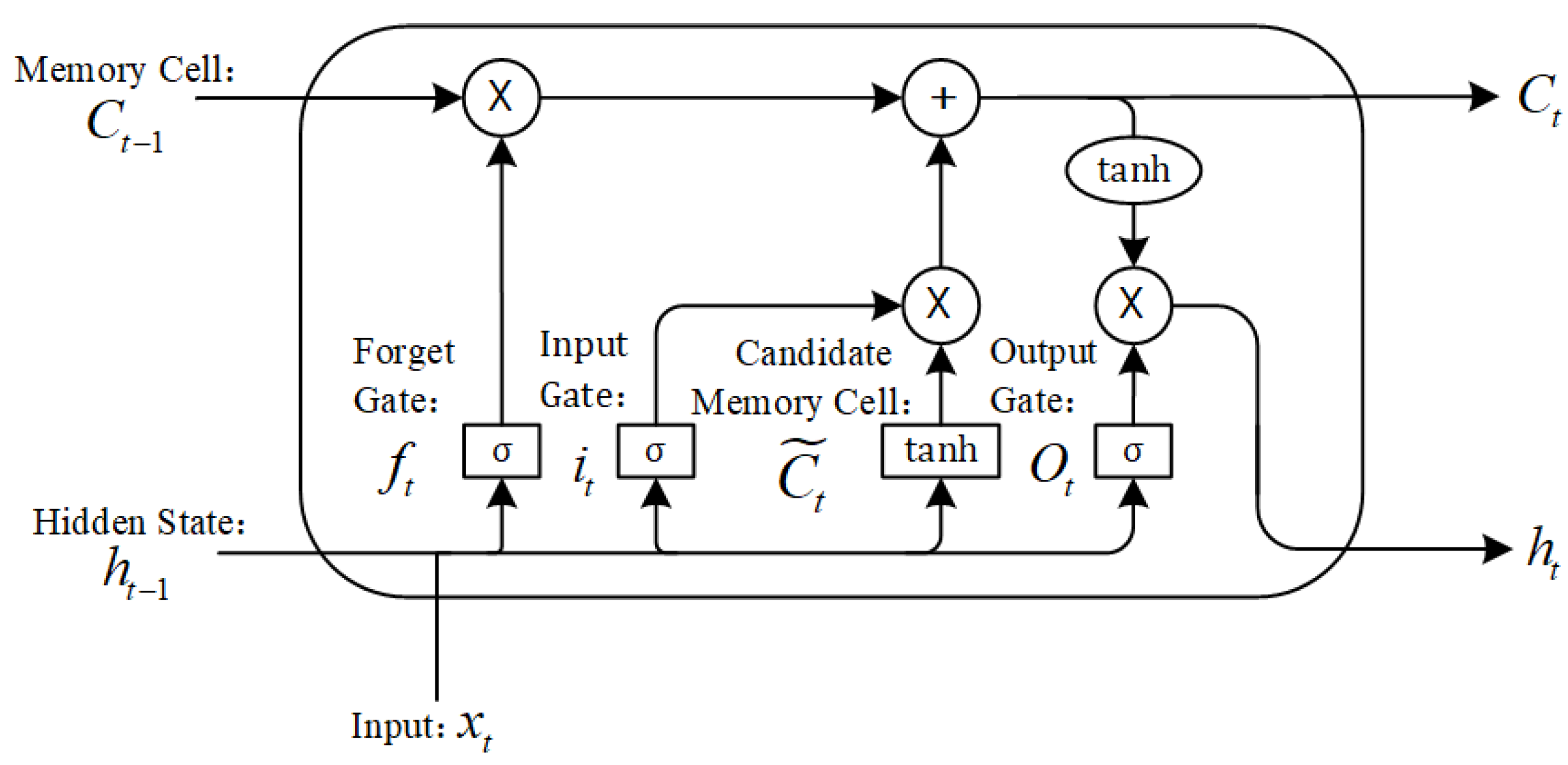
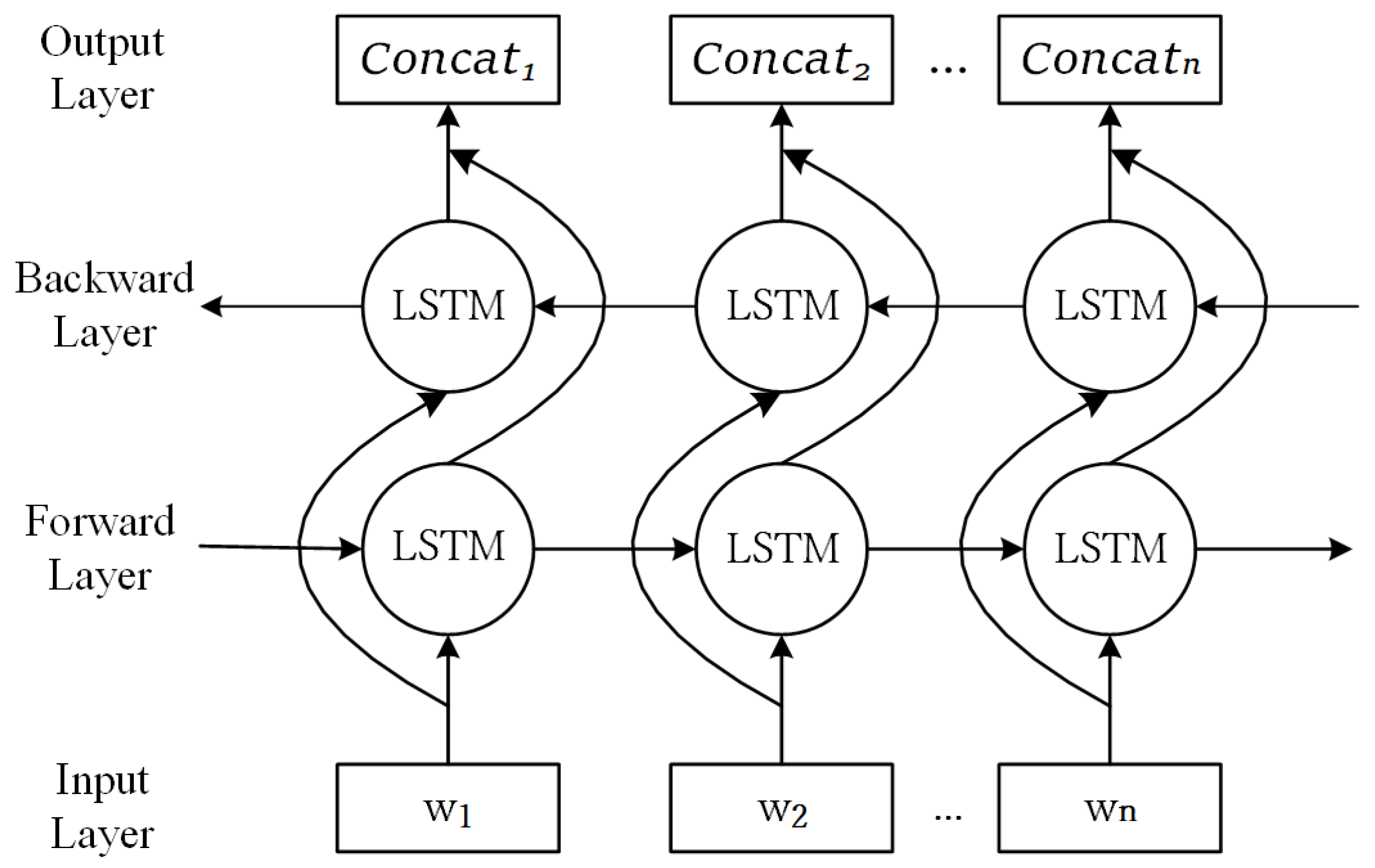
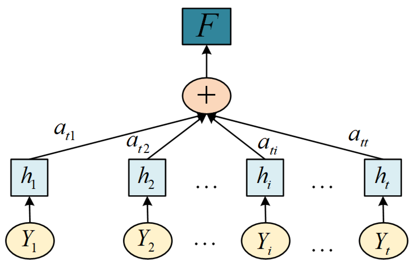
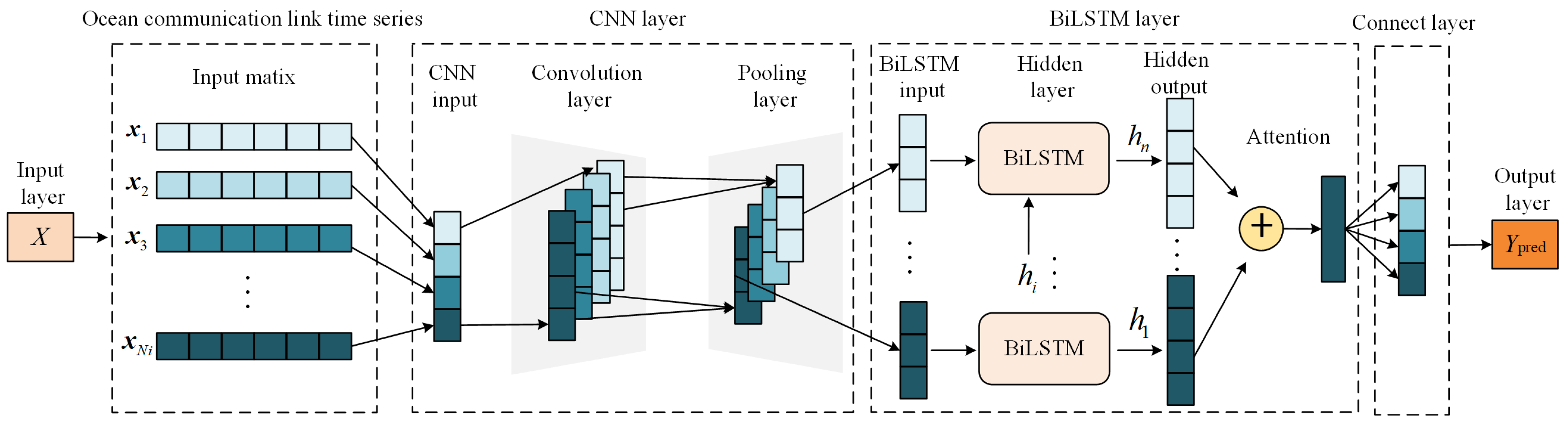
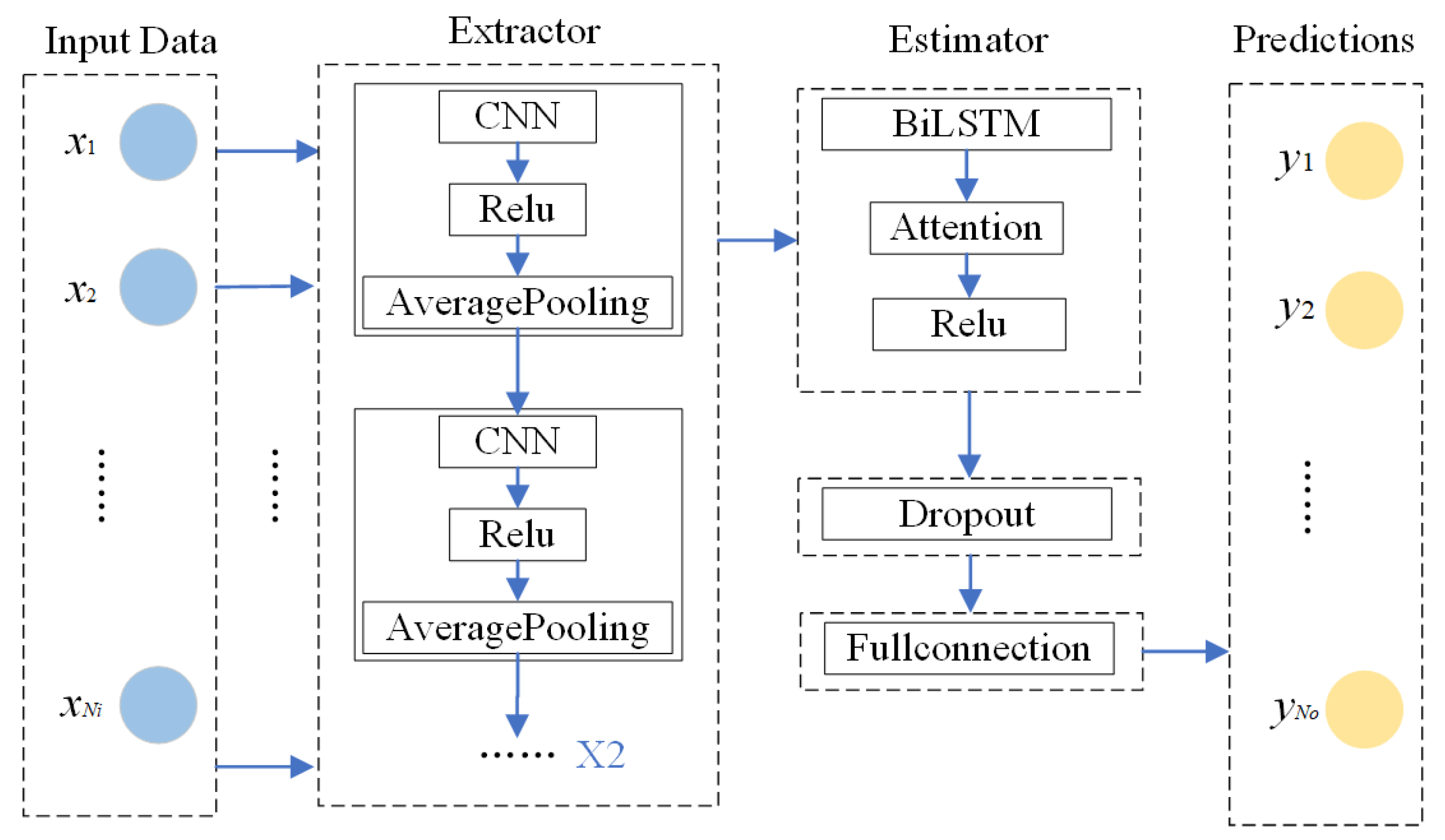
• A CNN-BiLSTM-AM cascade scheme is designed, where a CNN is used to extract the local features, BiLSTM is employed to model the long-term dependencies of the channel states, and an attention mechanism (AM) is introduced to adaptively focus on key node information. This approach achieves a high prediction accuracy.

2. The System Model

In the system model, a ship sailing near the shore is connected to an onshore base station through a relay ship, with both ships traveling at different speeds (v) along their respective routes, thereby forming a dynamic network environment. At two separate time instants $t_1$ and $t_2$, the positions of the ships and their communication connections change. This change mirrors the instability caused by the movement of ships in maritime communication networks. It is assumed that the decode-and-forward (DF) protocol is employed during this process. The link connection probability from the nearshore ship to the base station is calculated using the channel state information and marine environment parameters collected over the past $N_i$ time slots. A brief illustration of the system model is shown in Figure 1.

2.1. Wireless Channels

Wireless channels between any two nodes experience both large-scale path loss and small-scale fading. It is assumed that small-scale fading follows either a Rayleigh distribution or a Rician distribution, resulting in the received signal-to-noise ratio (SNR) following an exponential distribution. However, due to the ocean’s movement and weather variations, the channel model and its parameters are not stable, making the accurate estimation and collection of channel state information difficult.

The channel parameter $\lambda$ is used to characterize specific properties of the channel, such as fading and noise, and its value undergoes dynamic variations. To approximate the maritime wireless channel, it is assumed that the parameter of the exponential distribution $\lambda$ follows a certain random distribution, a uniform distribution, for instance, i.e., $\lambda \sim U({\lambda }_1,{\lambda }_u)$. This assumption effectively simulates the stochastic and bounded variability in maritime channels. The formulation of the channel model is presented as follows:

$$Y\left(t\right)=h\left(t\right)·\beta \left(t\right),$$

(1)

where $h\left(t\right)={\displaystyle \frac{1}{D^m}}$ signifies large-scale fading, m refers to the path loss exponent, D indicates the distance, and $\beta \left(t\right)$ signifies small-scale fading.

2.2. The Oceanic Environment

The main challenge in deploying wireless networks at sea is that hydrological and meteorological factors like wind and waves add stochastic fluctuations to the navigation status. The horizontal distances at the time point i between the two ships and between the relay ship and the BS are denoted by $d_i^1$ and $d_i^2$. Meanwhile, $h_i^1$ and $h_i^2$ represent the wave heights in the areas of the sea around the two respective ships. Thus, the exact distances are given by

$$d_i^1=\sqrt{{\left(d_i^1\right)}^2+{(h_i^1-h_i^2)}^2}$$

(2)

$$d_i^2=\sqrt{{\left(d_i^2\right)}^2+{\left(h_i^2\right)}^2}$$

(3)

$v_i^1$, $v_i^2$ represent the scalar speeds of the two ships at the i-th time instant, which are expressed as follows:

$$v_i^1=V_i^1+{\Delta }_i^1$$

(4)

$$v_i^2=V_i^2+{\Delta }_i^2$$

(5)

where ${\Delta }_i^1$, ${\Delta }_i^2$ are the associated random deviations and $V_i^1$, $V_i^2$ are the velocities recorded by the ship’s log-based instruments. ${\theta }_i^1$, ${\theta }_i^2$ signify the angles by which the actual cruising directions of the two ships deviate from the pre-defined nominal direction at the i-th time step.

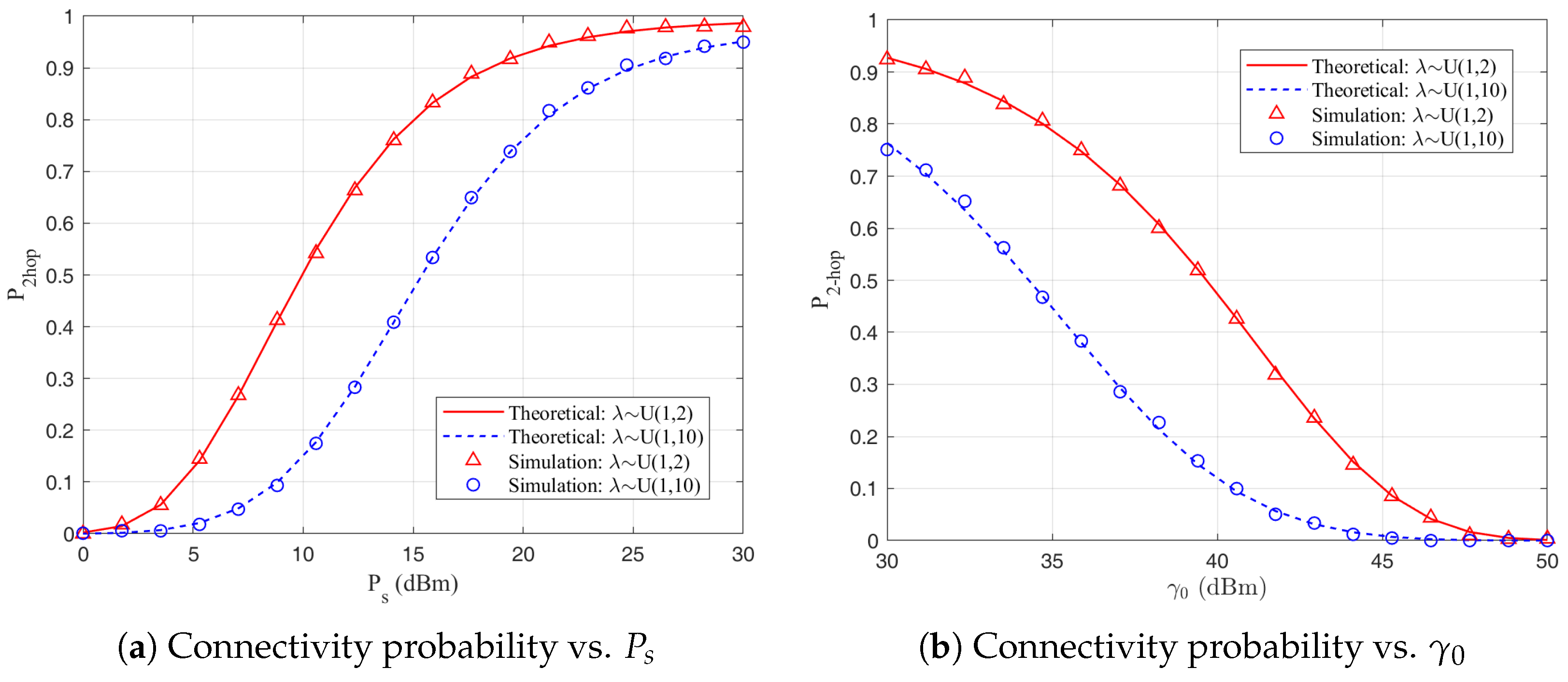
2.3. Connectivity Probability

Connectivity probability is one of the fundamental performance metrics in wireless communication systems. It is defined as the probability that the receiver successfully receives a signal with a signal-to-noise ratio (SNR) exceeding a specific threshold during signal transmission. Based on the wireless fading channel model described in Section 2.1, this paper primarily analyzes the distribution of the SNR and the connection probability under different path conditions, particularly in the case of Rayleigh fading. It is postulated that the channel gain ${\left|h\right|}^2\sim \exp \left(\lambda \right)$ at the receiver follows an exponential distribution. Therefore, its expression is given by

$${f\left(\right|h|}^2)=\lambda e^{-{\lambda \left|h\right|}^2},{\left|h\right|}^2\ge 0$$

(6)

where $\lambda$ is the parameter of the exponential distribution. In this case, the SNR of the signal transmission from the source to the relay node can be expressed as follows:

$${\mathrm{SNR}}_1={\displaystyle \frac{P_s{C}_1{d}_1^{-\alpha }{\left|h_{sr}\right|}^2}{n_0}}$$

(7)

The connection probability conditioned on ${\mathrm{SNR}}_1>{\gamma }_0$ is expressed as

$$P_y({\mathrm{SNR}}_1>{\gamma }_0)=P_y\left\{C_1{d}_1^{-\alpha }{\displaystyle \frac{P_s{\left|h_{sr}\right|}^2}{n_0}}>{\gamma }_0\right\}$$

(8)

where $P_s$ is the transmission power of the shore-based source, $C_1$ is the path loss factor from the source to the relay node, $d_1$ is the distance between the source and the relay node, $\alpha$ is the path loss exponent, ${\gamma }_0$ is the target SNR threshold, and $n_0$ is the noise power.

Assuming that the parameter $\lambda$ is uniformly distributed within the interval $[a,b]$ to simulate offshore channel conditions under different scenarios, its distribution is given by

$$f\left(\lambda \right)={\displaystyle \frac{1}{b-a}},\lambda \in [a,b]$$

(9)

Substituting the above expression, the conditional probability expression can be obtained as follows:

$$P_y({\mathrm{SNR}}_1>{\gamma }_0)={\int }_a^b{\int }_{{\displaystyle \frac{{\gamma }_0{n}_0}{P_s{C}_1{d}_1^{-\alpha }}}}^{\infty }{\displaystyle \frac{\lambda e^{-\lambda x}}{b-a}}dxd\lambda$$

(10)

By integrating with respect to ${\left|h\right|}^2$ and $\lambda$, the expression can be further simplified as

$$\begin{gathered} P_y={\int }_a^b{\displaystyle \frac{1-F\left(x\right)}{b-a}}d\lambda ={\int }_a^b{\displaystyle \frac{e^{-\lambda \frac{{\gamma }_0{n}_0}{P_s{C}_1{d}_1^{-\alpha }}}}{b-a}}dxd\lambda \\ ={\displaystyle \frac{1}{b-a}}{\displaystyle \frac{P_s{C}_1{d}_1^{-\alpha }}{{\gamma }_0{n}_0}}\left(e^{-a{\displaystyle \frac{{\gamma }_0{n}_0}{P_s{C}_1{d}_1^{-\alpha }}}}-e^{-b{\displaystyle \frac{{\gamma }_0{n}_0}{P_s{C}_1{d}_1^{-\alpha }}}}\right) \end{gathered}$$

(11)

where $F\left(x\right)$ is the cumulative distribution function (CDF) of the received signal and is expressed as an exponential distribution: $F\left(x\right)=1-e^{-\lambda x},(x>0)$.

Similarly, the probability expression for the second hop, where ${\mathrm{SNR}}_2>{\gamma }_0$, can be derived as

$$\begin{gathered} P_y({\mathrm{SNR}}_2>{\gamma }_0)={\int }_a^b{\int }_{{\displaystyle \frac{{\gamma }_0{n}_0}{P_r{C}_2{d}_2^{-\alpha }}}}^{\infty }{\displaystyle \frac{\lambda e^{-\lambda x}}{b-a}}dxd\lambda \\ ={\displaystyle \frac{1}{b-a}}{\displaystyle \frac{P_r{C}_2{d}_2^{-\alpha }}{{\gamma }_0{n}_0}}\left(e^{-a{\displaystyle \frac{{\gamma }_0{n}_0}{P_r{C}_2{d}_2^{-\alpha }}}}-e^{-b{\displaystyle \frac{{\gamma }_0{n}_0}{P_r{C}_2{d}_2^{-\alpha }}}}\right) \end{gathered}$$

(12)

where $P_r$ is the transmission power at the relay node, $C_2$ is the path loss factor from the relay node to the receiving end, and $d_2$ is the distance from the relay node to the target node.

Relay cooperative communication techniques are primarily categorized into amplify-and-forward (AF) and decode-and-forward (DF) schemes based on their signal processing methods. In the AF mode, the relay nodes directly amplify and forward the noisy source signal without performing demodulation or decoding. Conversely, the DF mode involves the relay nodes demodulating and decoding the received signal first, followed by re-encoding and modulating it before its transmission to the destination node [18]. In a harsh noise environment, since the DF mode can remove noise through decoding, compared with the AF mode, it performs better in ensuring the signal quality and transmission reliability and can effectively reduce the bit error rate of wireless communication. Based on this, the decode-and-forward mechanism is adopted in this work. For a two-hop communication system, the system’s connection probability depends on the channel conditions of each hop. The signal-to-noise ratio of the entire system is determined by the minimum SNR of the two hops. Thus, the overall system SNR is expressed using the following formula:

$$SN{R}_{e2e}=min\left[{\displaystyle \frac{P_s{\left|h_{sr}\right|}^2}{P_n}},{\displaystyle \frac{P_r{\left|h_{rd}\right|}^2}{P_n}}\right]$$

(13)

Therefore, the connection probability of the two-hop communication system can be expressed as

$$P_{2hop}=P(min[SN{R}_1,SN{R}_2]>{\gamma }_0)=P(SN{R}_1>{\gamma }_0)·P(SN{R}_2>{\gamma }_0)$$

(14)

Further derivations can be made:

$$\begin{gathered} P_{2\mathrm{hop}}={\left({\displaystyle \frac{1}{b-a}}\right)}^2\left\{{\displaystyle \frac{P_s{C}_1{d}_1^{-\alpha }}{{\gamma }_0{n}_0}}\left(e^{-a{\displaystyle \frac{{\gamma }_0{n}_0}{P_s{C}_1{d}_1^{-\alpha }}}}-e^{-b{\displaystyle \frac{{\gamma }_0{n}_0}{P_s{C}_1{d}_1^{-\alpha }}}}\right)\right\} \\ ·\left\{{\displaystyle \frac{P_r{C}_2{d}_2^{-\alpha }}{{\gamma }_0{n}_0}}\left(e^{-a{\displaystyle \frac{{\gamma }_0{n}_0}{P_r{C}_2{d}_2^{-\alpha }}}}-e^{-b{\displaystyle \frac{{\gamma }_0{n}_0}{P_r{C}_2{d}_2^{-\alpha }}}}\right)\right\} \end{gathered}$$

(15)

The connection probability of a two-hop system, as indicated in (15), is determined by various parameters. These include the distribution trend in the received channel gain, the path loss for each hop, distance, transmission power, forwarding power, noise power, and the signal-to-noise ratio threshold.

However, in real-world maritime wireless communication networks, various dynamic environmental conditions can significantly affect the accuracy of the connection probability calculations. The impact of factors such as the ship’s speed, surface wave fluctuations, and weather conditions on the system performance remains unclear. As a result, the validity of existing models requires further evaluation and refinement. To tackle this challenge, it is essential to develop a novel data-driven framework tailored to wireless networks operating in complex maritime environments.

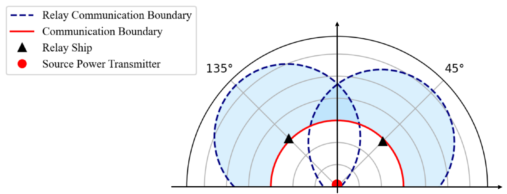
2.4. The Coverage Area

By introducing relay ships to forward the signals, the coverage range between remote ships and shore stations can be significantly expanded, thus improving the reach and stability of communication. Based on the assumption in Section 2.3, the probability of (SNR > ${\gamma }_0$) in traditional single-hop networks is given by

$$P_y=P\left\{{\left|h\right|}^2>{\displaystyle \frac{n_0{\gamma }_0}{P_s{C}_0{d}_0^{-\alpha }}}\right\}=e^{-\lambda {\displaystyle \frac{n_0{\gamma }_0}{P_s{C}_0{d}_0^{-\alpha }}}}$$

(16)

Comparing the performance of traditional single-hop and dual-hop schemes, the following condition is obtained:

$$P_{2hop}>P_y\to e^{-n_0{\gamma }_0}\left({\displaystyle \frac{{\lambda }_1}{P_s{C}_1{d}_1^{-\alpha }}}+{\displaystyle \frac{{\lambda }_2}{P_r{C}_2{d}_2^{-\alpha }}}\right)>e^{-n_0{\gamma }_0{\displaystyle \frac{{\lambda }_0}{P_s{C}_0{d}_0^{-\alpha }}}}$$

(17)

Simplifying the equation leads to

$${\displaystyle \frac{{\lambda }_1}{P_s{C}_1{d}_1^{-\alpha }}}+{\displaystyle \frac{{\lambda }_2}{P_r{C}_2{d}_2^{-\alpha }}}<{\displaystyle \frac{{\lambda }_0}{P_s{C}_0{d}_0^{-\alpha }}}$$

(18)

The above formula demonstrates a condition under which the dual-hop channel outperforms the traditional single-hop channel, considering changes in the channel conditions and relay configuration parameters.

Based on the derived formula, this paper uses Figure 2 to show the coverage area of a dual-hop communication system in polar coordinates compared to that of a traditional single-hop communication system. The red dot in the figure marks the position of the source transmitter, typically the shore station. The triangle symbol represents the relay ship’s position, acting as an intermediate node in the signal transmission path. The solid line area represents the maximum coverage area directly connected to the source transmitter. The light blue-shaded region indicates the extended range achievable through relay transmission. This illustrates that compared to traditional single-hop communication, the dual-hop system can extend its coverage and achieve more stable communication.

3. Principles of the Deep Learning Models

3.1. The CNN-BiLSTM Model

Lu et al. [19] proposed the CNN-LSTM hybrid model, where a convolutional neural network (CNN) is a multi-layer neural network structure with a deep supervised learning architecture capable of handling time-series and image data. The role of the CNN is to extract the signal features from the received signals and then integrate these extracted features into a two-dimensional array, which is subsequently passed as input to the LSTM layer to analyze the feature information in the time series of the received signals. Unlike the single CNN model, which can only extract local features, the CNN-LSTM fusion model offers more comprehensive feature extraction capabilities and demonstrates a significant improvement in time-series modeling thanks to LSTM’s effective modeling of the temporal dependencies. Compared to the standalone LSTM model, CNN-LSTM shows greater applicability and higher computational efficiency when handling high-dimensional time-series data. In this architecture, the CNN first performs dimensionality reduction on the data and extracts key features, significantly reducing the input data dimensions that need to be processed by the subsequent LSTM step. This approach not only accelerates the model training process but also effectively reduces the overall computational complexity.

Long short-term memory (LSTM) networks effectively regulate the flow of information by introducing three unique gating mechanisms, the forget gate, the input gate, and the output gate, which improve the network’s ability to handle long-term dependencies. The specific network structure of the LSTM model is shown in Figure 3.

Here, the input at each time step is represented by $x_t$, and the core component $C_t$ (the memory unit) plays a crucial role in LSTM, responsible for maintaining the state information across time steps. The dynamics of the LSTM unit can be described by the following equations:

$$i_t=\sigma (W_{xi}{x}_t+W_{hi}{h}_{t-1}+b_i)$$

(19)

$$f_t=\sigma (W_{xf}{x}_t+W_{hf}{h}_{t-1}+b_f)$$

(20)

$$o_t=\sigma (W_{xo}{x}_t+W_{ho}{h}_{t-1}+b_o)$$

(21)

$${\tilde{c}}_t=tanh(W_{xc}{x}_t+W_{hc}{h}_{t-1}+b_c)$$

(22)

$$c_t=f_{t}e{c}_{t-1}+i_{t}e{\tilde{c}}_t$$

(23)

$$h_t=o_{t}etanh\left(c_t\right)$$

(24)

Here, $\sigma$ represents the sigmoid activation function; tanh represents the hyperbolic tangent activation function, as shown in Equations (25) and (26). The input gate controls the input of new information, and the forget gate determines which information in the memory unit should be forgotten, while the output gate controls the output to the next state of the LSTM unit. Other variants of recurrent neural networks (RNNs), such as Gated Recurrent Units (GRUs), have a relatively simpler structure, consisting only of a reset gate and an update gate. However, due to the reduced state control capability of the gating mechanism, their performance is inferior to that of LSTM networks when handling long-sequence data.

$$\sigma \left(x\right)={\displaystyle \frac{1}{1+e^{-x}}}$$

(25)

$$tanh\left(x\right)={\displaystyle \frac{e^x-e^{-x}}{e^x+e^{-x}}}$$

(26)

In comparison with the LSTM model, this paper employs the BiLSTM model, which has significant advantages in processing sequential data. The structure of the BiLSTM network is shown in Figure 4.

Here, w is the trainable weight matrix. As can be seen in Figure 3, the BiLSTM network is composed of two LSTM networks: one is the forward LSTM network, which calculates the forward hidden states (${\overrightarrow{h}}_1,\cdots ,{\overrightarrow{h}}_s$) of the sequence; the other is the backward LSTM network, which calculates the backward hidden states (${\overleftarrow{h}}_1,\cdots ,{\overleftarrow{h}}_s$). By integrating the hidden states from both directions at each time step, the network effectively combines the forward and backward feature information. Finally, these fused hidden states H are used as features and passed on to subsequent layers for further processing. In contrast, unidirectional LSTM can only retain past information, while the design of bidirectional LSTM allows the model to not only capture the impact of historical information on the current state but also to proactively consider the influence of future information.

3.2. The Attention Mechanism

The attention mechanism (AM) is inspired by the simulation of the attention characteristics of the human brain and is an important tool for addressing the issue of information overload [20]. It has been widely applied in the field of deep learning. The fundamental principle of the AM is to allocate weights based on the varying impact of the input features on the output results, thereby enhancing the model’s feature extraction capability through differentiated weights. In this paper, the AM first generates feature representations from the hidden states of the previous layer (i.e., the BiLSTM layer) and calculates the importance scores for each time step using a trainable weight matrix. Subsequently, the scores are normalized using the Softmax function to obtain the weights for each time step. These weights are then used to perform a weighted sum of the hidden states to generate the context vector, which highlights the significant temporal features. During the training process, the AM dynamically adjusts the weight distribution by optimizing the network parameters, improving the model’s ability to capture non-linear relationships while also enhancing its robustness and generalization capability. The structure of the AM unit is shown in Figure 5.

The attention state transformation process is shown in Equations (27)–(29):

$$S_{ti}=Vtanh(W{h}_t+U{h}_i+b),i=1,2,\cdots ,t-1$$

(27)

$$a_{ti}={\displaystyle \frac{exp\left(S_{ti}\right)}{{\sum }_{i=1}^{t}exp\left(S_{tk}\right)}},i=1,2,\cdots ,t-1$$

(28)

$$F=\sum _{i=1}^t{a}_{ti}\times h_i,i=1,2,\cdots ,t-1$$

(29)

In the above equations, V, W, U, and b are the network model parameters; $h_i$ is the hidden state of the corresponding input sequence $Y_i$; and $a_{ti}$ is the weight of the BiLSTM hidden state $h_i$ with respect to the current input $Y_i$. And F is the attention layer’s output. The overall workflow for CNN-BiLSTM-AM is shown in Figure 6.

4. A Connectivity Analysis Based on the CNN-BiLSTM-AM Model

The structure of the proposed method is depicted in Figure 7. The CNN module, which functions as the feature extractor, comprises a four-layer architecture. A linear rectified activation function (ReLU) is applied after each layer to enhance its ability to model non-linear relationships. Additionally, an average pooling layer is incorporated to reduce the number of parameters and mitigate the risk of overfitting. Specifically, the module can automatically capture and abstract implicit features that influence the ship–shore connectivity—for instance, the movement direction, speed, distance, signal-to-noise ratio, and other key factors, as well as the latent feature patterns among these critical variables. Consequently, the CNN is capable of extracting effective high-level features from complex input data, which are subsequently passed as input to the BiLSTM module.

Given the constantly changing conditions of the maritime environment and the movement of ships, these factors present considerable difficulties for network connectivity analyses. To address this, the proposed approach leverages historical time-series data for the analysis. By leveraging the memory mechanism and long-sequence learning capability of BiLSTM networks, the model further explores the dependencies and dynamic change patterns along the temporal dimension and computes the connectivity probability over the time series.

Subsequently, an AM is introduced to distinguish the significance of the time-related information extracted from the BiLSTM hidden layers. This weighted aggregation process enables the model to uncover deeper temporal features within the response data. Finally, a Dropout layer is applied as a regularization technique to prevent overfitting. By randomly deactivating certain neurons (including both hidden and visible layers) during training, Dropout facilitates a more robust learning environment for the multi-layer perceptron. It accelerates training, reduces the computational demands, and shortens the training time. The final fully connected layer is responsible for generating the output results.

4.1. Input–Output Data

Considering the impact of the marine environment, hydrological and meteorological parameters such as humidity and the signal-to-noise ratio can be measured by the receiver, with both historical and current data accessible. These data are used as input features, including the channel properties, marine environmental conditions, and ship navigation parameters, which are all obtained via measurements. The input data X are defined by Equation (30) as follows:

$$\mathit{X}=({\mathit{x}}_{\mathbf{1}},{\mathit{x}}_{\mathbf{2}},\cdots ,{\mathit{x}}_{{\mathit{N}}_{\mathit{i}}})$$

(30)

Each feature is a vector that includes multiple parameters collected at a specific time point.

$${\mathbf{x}}_{\mathbf{i}}=\left(v_i^1,v_i^2,{\theta }_i^1,{\theta }_i^2,d_i^1,d_i^2,{\gamma }_i^1,{\gamma }_i^2,h_i^1,h_i^2\right)$$

(31)

• Speed:
  ${\mathbf{v}}_{\mathbf{1}}=[v_1^1,v_2^1,\cdots ,v_{N_i}^1]$, ${\mathbf{v}}_{\mathbf{2}}=[v_1^2,v_2^2,\cdots ,v_{N_i}^2]$
• Direction Angles:
  ${\theta }_{\mathbf{1}}=[{\theta }_1^1,{\theta }_2^1,\cdots ,{\theta }_{N_i}^1]$, ${\theta }_{\mathbf{2}}=[{\theta }_1^2,{\theta }_2^2,\cdots ,{\theta }_{N_i}^2]$
• Distance:
  ${\mathbf{d}}_{\mathbf{1}}=[d_1^1,d_2^1,\cdots ,d_{N_i}^1]$, ${\mathbf{d}}_{\mathbf{2}}=[d_1^2,d_2^2,\cdots ,d_{N_i}^2]$
• Signal-to-Noise Ratio:
  ${\mathit{\gamma }}_{\mathbf{1}}=[{\gamma }_1^1,{\gamma }_2^1,\cdots ,{\gamma }_{N_i}^1]$, ${\mathit{\gamma }}_{\mathbf{2}}=[{\gamma }_1^2,{\gamma }_2^2,\cdots ,{\gamma }_{N_i}^2]$
• Wave Height:
  ${\mathbf{h}}_{\mathbf{1}}=[h_1^1,h_2^1,\cdots ,h_{N_i}^1]$, ${\mathbf{h}}_{\mathbf{2}}=[h_1^2,h_2^2,\cdots ,h_{N_i}^2]$

The problem of maritime wireless communication connectivity analysis is addressed by predicting the future ship-to-shore connectivity based on historical marine environmental data. The output data $\mathbf{Y}$ are represented as

$$\mathit{Y}=[{\mathit{y}}_{\mathbf{1}},{\mathit{y}}_{\mathbf{2}},\cdots ,{\mathit{y}}_{{\mathit{N}}_{\mathit{o}}}]$$

(32)

where ${\mathit{y}}_{\mathit{i}}$ indicates the estimated connection probability of the two-hop link at the i-th time slot. The total number of output data points is $N_o$, meaning that the method predicts the connection probability at $N_o$ different time instances.

4.2. The Data Generation Method

In maritime networks, vast historical datasets are generated during navigation, which can be used as samples for training. However, in this study, collecting these data within a short period is neither cost-effective nor feasible. To assess the effectiveness of the proposed algorithm and reduce the experimental costs, this paper designs a software-assisted data generation method to implement the channel model presented in Section 2 while simultaneously generating the navigation and hydrological parameters. Based on these data, the input data and output labels are generated and packaged into training and prediction sample sets. The following is a overview of Algorithm 1 in this method.

Algorithm 1 Approach to Data Generation

Step 1: Input Data Generation     0. Parameter Initialization     1.1 Generation of Received Signal-to-Noise Ratios (SNRs)        Generate an instance of $\lambda$ through the uniform distribution $U({\lambda }_l,{\lambda }_u)$. This distribution models the bounded random fluctuations in the channel conditions.        Generate the signal-to-noise ratios ${\gamma }_{\mathbf{1}}$ and ${\gamma }_{\mathbf{2}}$ using an exponential distribution with the parameter $exp\left(\lambda \right)$, aligning with the Rayleigh fading model theoretically.     1.2 Generate ${\mathit{d}}_{\mathbf{1}}$, ${\mathit{d}}_{\mathbf{2}}$ using the uniform distribution $U(d_l,d_u)$. This distribution represents the spatial randomness of the deployment of nodal ships within a pre-defined operational area.     1.3 Generate ${\mathit{h}}_{\mathbf{1}}$ and ${\mathit{h}}_{\mathbf{2}}$ using the normal distribution $N(\mu ,{\sigma }^2)$. This distribution is commonly applied in oceanography to modeling the variability in the wave heights under diverse sea conditions.     1.4 Generate ${\mathit{v}}_{\mathbf{1}}$, ${\mathit{v}}_{\mathbf{2}}$, and ${\theta }_{\mathbf{1}}$, ${\theta }_{\mathbf{2}}$ using the uniform distribution $U(v_l,v_u)$, $U({\theta }_l,{\theta }_u)$. These distributions capture the random characteristics of nodal ship movement while adhering to environmental and operational limitations.     1.5 Pack data         Repeat steps 1.1 to 1.4 for a total of 20,000 iterations.         Reorganize all the data and package them into $\mathit{X}=[{\mathit{X}}_{\mathit{t}},{\mathit{X}}_{\mathit{p}}]$, where ${\mathit{X}}_{\mathit{t}}$ is the data used for training the model, and ${\mathit{X}}_{\mathit{p}}$ is the data for prediction. Step 2: Output Data Generation      2.1 Use the Monte Carlo method to compute the connection probability for $\mathit{X}$.        The computed result is packaged into $\mathit{Y}=[{\mathit{Y}}_{\mathit{t}},{\mathit{Y}}_{\mathit{p}}]$, where ${\mathit{Y}}_{\mathit{t}}$ is the connection probability for the training data, and ${\mathit{Y}}_{\mathit{p}}$ is the connection probability for the prediction data. Step 3: Predict the Connection Probability      3.1 Package the training datasets $[{\mathit{X}}_{\mathit{t}},{\mathit{Y}}_{\mathit{t}}]$ and train the network.      3.2 Feed input ${\mathit{X}}_{\mathit{p}}$ into the network to derive the predicted output ${\mathit{Y}}^{\prime }$.      3.3 Compare ${\mathit{Y}}_{\mathit{p}}$ with ${\mathit{Y}}^{\prime }$ to calculate the error.

5. The Experimental Results and Evaluation Metrics

5.1. The Experimental Environment

The experimental environment was as follows: The operating system was Windows 10, the CPU was an AMD Ryzen7 5800H, the memory size was DDR4 16 GB, and the development tool used was MATLAB R2022b.

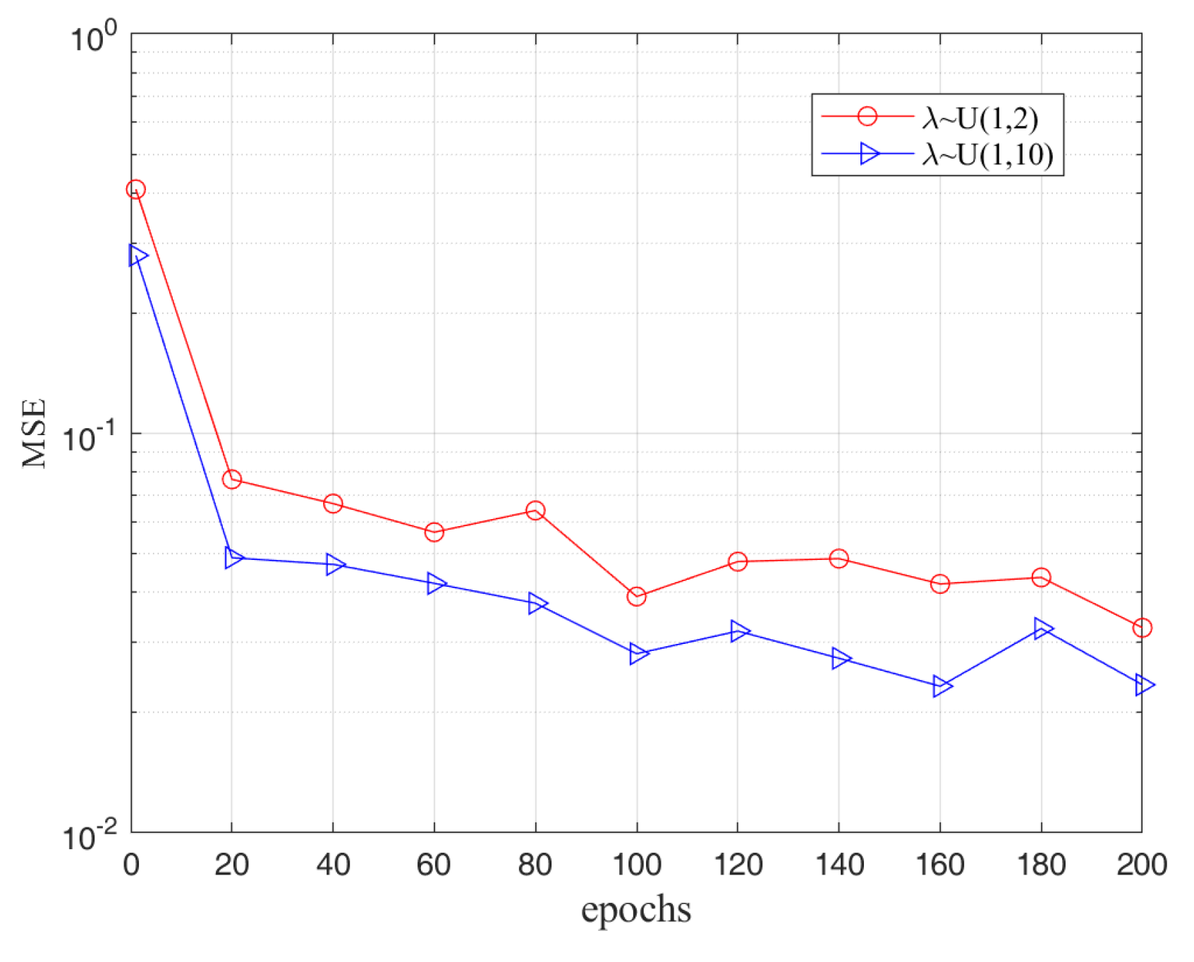
5.2. Analysis of the Results

The simulation was performed using MATLAB R2022b to generate the raw data, which were derived by modeling essential channel characteristics in the maritime communication environment, including the large-scale path loss and Rayleigh fading.

Table 1. Marine wireless communication environment and dataset parameters.

Category	Parameter	Value
Marine communication	Maximum sea wave height	2 m
	Average sea wave height	1.5 m
Transmitter and receiver	Transmission power	15–30 dBm
	Carrier frequency	5.8 GHz
	Transmit antenna height	12 m
	Receive antenna height	8 m
	Sound power	2–4 dBm
Ship movement	Sampling interval	120 s
	Distance	10–20 km
	Speed	$0\le v\left(t\right)\le 30$ km/h
	Direction	$-{\displaystyle \frac{\pi }{6}}\le \theta \left(t\right)\le {\displaystyle \frac{\pi }{6}}$

lists the configuration of the main communication parameters and dataset parameters.

Before model training, each data group must be labeled with its corresponding connection probability as the target. The complete dataset is then split into training and testing sets at an 8:2 ratio. The specific network parameters and hyperparameter settings of the CNN-BiLSTM-AM network are presented in

Table 2. CNN-BiLSTM-AM neural network parameter settings.

	Parameter	Value
Input layer	Number of nodes	20K × 10
CNN layer	Filter 1: size/number/stride	3/6/1
	Filter 2: size/number/stride	3/12/1
	Filter 3: size/number/stride	3/32/1
	Filter 4: size/number/stride	3/64/1
	Pooling type/kernel size/stride	AveragePooling/2/1
	Activation function	ReLU
BiLSTM layer	Number of LSTM units (forward)	32
	Number of LSTM units (backward)	32
	Dropout parameter	0.2
Attention layer	Activation function	Softmax
Output layer	Number of nodes	20K × 1
Hyperparameters	Optimizer	Adam
	Batch size	32
	Epochs	200
	Learning rate	0.01

. The Adam optimizer was employed to optimize the network parameters. The batch size is set to 32 to reduce the memory usage and prevent overfitting. The maximum number of training epochs is set to 200, with an initial learning rate of 0.01. A step-by-step decay strategy is adopted, halving the learning rate every 20 epochs. This strategy helps to accelerate convergence in the early stages of training, avoid gradient explosion, and stabilize the model training process by gradually decreasing the learning rate in the later stages [21].

To verify the congruence between the theoretical values and the simulation results regarding the connectivity probability, Figure 8 depicts the connectivity probability under diverse system parameters. In the two figures, the solid and dashed lines represent the theoretical values of the results obtained when the distribution parameters of the signal-to-noise ratio follow different distributions in order to simulate various channel conditions. The triangle and circle markers correspond to the simulation results obtained through the data generation method. In Figure 8a, where $\lambda$ follows a uniform distribution $U(1,2)$ and the transmission power $\lambda$ is 24 dBm, the theoretical values and the simulated results show a maximum deviation of only 1.22%. In contrast, when $\lambda$ follows a uniform distribution $U(1,10)$, the transmission power $\lambda$ is 27 dBm, and the theoretical values show a maximum deviation of 1.81% compared to the simulated results. In Figure 8b, the maximum difference between the theoretical analysis and the simulation results is only 1.65%. Overall, the high degree of consistency observed between the theoretical and simulation results attests to the precision of the formulas and the dependability of the methods.

In Figure 8a, when $\lambda$ follows a uniform distribution $U(1,2)$, as the transmission power $P_s$ increases from 5 to 15 dBm, the connection probability $P_{2hop}$ shows a rapid increase. Especially at lower transmission powers, the system’s performance improves significantly. However, when $\lambda$ follows $U(1,10)$, as the transmission power $P_s$ increases from 5 to 15 dBm, the connection probability $P_{2hop}$ shows a more gradual increase, indicating that the expansion of the channel attenuation range has a more significant negative impact on the system performance.

In Figure 8b, it can be observed that regardless of whether $\lambda$ follows $U(1,2)$ or $U(1,10)$, as the signal-to-noise ratio threshold ${\gamma }_0$ increases, the connection probability gradually decreases, indicating that the system becomes more stringent for a higher ${\gamma }_0$, and the power cost required to meet the requirements also increases. It is noteworthy that when the signal-to-noise ratio threshold ${\gamma }_0$ exceeds 45 dBm, the decline in the connection probability tends to stabilize, suggesting that the system performance becomes stable after this point.

The model’s accuracy is assessed by comparing the predicted labels of the test set with the actual outputs, using the mean squared error (MSE) as the evaluation metric. For time-series prediction tasks, the error can be calculated to evaluate the final model’s effectiveness. The definition of the MSE is as follows:

$$M_{\mathrm{MSE}}(y,\widehat{y})={\displaystyle \frac{1}{n}}\sum _{i=1}^n{(y_i-{\widehat{y}}_i)}^2$$

(33)

where y represents the true values; $\widehat{y}$ represents the predicted results of the sample; and n represents the number of samples.

Three sets of experiments were designed, each with different parameter configurations, to evaluate the predictive performance of the model. The following presents a detailed analysis and the experimental results.

Figure 9 illustrates the MSE of the proposed scheme under the Rayleigh fading assumption, when the channel gain coefficients follow different distributions. It can be observed that the curve reaches its minimum value at the 200th iteration, and the MSE value gradually converges at 0.05 and 0.03, respectively. When $\lambda$ follows a uniform distribution $U(1,2)$, the MSE is relatively higher, which is due to the small range of fluctuations limiting the diversity of the sample, thus affecting the model’s ability to generalize, leading to a reduction in the performance.

Figure 10 demonstrates the trend in the variation in the MSE with respect to the output sequence’s length $N_o$, where $N_o$ is set to 1, 4, and 8. It can be observed that when $N_o=1$, the MSE is minimized. The curves gradually converge at 0.05, 0.03, and 0.01, respectively. This indicates that a larger $N_o$ value results in relatively higher MSE. The reason for this lies in the extension of the prediction time span, which increases the difficulty of calculating the connection probabilities. To select the most appropriate $N_o$ value, it is necessary to balance the MSE performance and maintain the prediction accuracy.

In contrast to terrestrial systems, maritime communication systems are substantially more influenced by the environmental conditions. Among these, wave height stands out as one of the crucial factors that has an impact. Figure 11 shows the change in the MSE with varying wave heights. Under Rayleigh fading, the difference in the MSEs for different wave heights reaches 0.06. It can be inferred that the Rayleigh fading channel exhibits strong sensitivity to wave height. Moreover, when the region is affected by larger ocean waves, that is, greater wave heights result in more signal fluctuation and instability due to the harsher transmission conditions, thereby increasing the MSE. On the other hand, lower wave heights create a more stable transmission environment, enhancing the signal quality and reducing the MSE. When compared to the influence of the $\lambda$ parameters on the MSE, wave height mainly impacts the physical stability of the signals. In contrast, Rayleigh fading brings about statistical variations in the channel conditions. Evidently, both factors exert a notable influence on the system performance, underscoring the importance of accounting for environmental variability in designing robust maritime communication systems.

The experimental results demonstrate that the model proposed in this paper can automatically capture and analyze the potential impact of environmental factors, such as ocean waves, on the characteristics of wireless communication channels. Moreover, it makes corresponding adjustments during the actual prediction process, enhancing the accuracy of the predictions and the robustness of the system. This method not only strengthens the system’s ability to cope with complex environmental changes but also highlights its application potential in dynamic maritime communication scenarios.

5.3. Model Comparison

To verify the performance of the CNN-BiLSTM-AM fusion model proposed in this study, we conducted comparative experiments between the proposed model and a single CNN model, a single BiLSTM model, the traditional machine learning method Support Vector Machine (SVM), and other deep learning models. A total of 2K samples were extracted from the test set (the marine communication link dataset) as the experimental data, and all of the models were evaluated under the same experimental conditions and parameter settings for prediction. The performance in link prediction was assessed using three metrics, the mean squared error (MSE), the mean absolute error (MAE), and the coefficient of determination (R²), while the inference time was used to evaluate the computational complexity and performance cost of the models. The calculation formulas for each error index are presented as follows:

$$MAE(y,\widehat{y})={\displaystyle \frac{1}{n}}\sum _{i=1}^n|y_i-{\widehat{y}}_i|$$

(34)

$$R^2=1-{\displaystyle \frac{{\sum }_{j=1}^N{[\widehat{y}\left(i\right)-y\left(i\right)]}^2}{{\sum }_{j=1}^N{[y\left(i\right)-\overline{y}]}^2}}$$

(35)

As shown in

Table 3. Comparison of single models with the fusion model.

Method	MSE (10−2)	MAE (10−2)	R2 (%)	Inference Time (s)
CNN	22.49	45.12	87.24	34
BiLSTM	10.13	29.78	95.13	90
CNN-BiLSTM-AM	1.26	10.23	97.98	101

, the MSE of the proposed fusion model improved by 0.2123 and 0.0887 compared to that of the single CNN and single BiLSTM models, respectively. Furthermore, the R² value of the proposed model reached 97.98%, close to 1, indicating a high level of fit. By leveraging the CNN to extract the local features of the sequence and BiLSTM for global temporal modeling, the fusion of these two complementary models resulted in a higher prediction accuracy than that of any single model.

This paper conducts a comparison not only with a single model but also traditional machine learning algorithms, such as SVM and other deep learning models. The experimental results are shown in

Table 4. Comparison of other models with the fusion model.

Method	MSE (10−2)	MAE (10−2)	R2 (%)	Inference Time (s)
SVM	41.27	62.20	78.61	15
CNN-RNN	8.39	25.97	96.95	75
CNN-GRU	6.47	23.44	97.04	83
CNN-BiLSTM-AM	1.26	10.23	97.98	101

. The MSE, MAE, and R² of the CNN-BiLSTM-AM model are 0.0126, 0.1023, and 97.98%, respectively, demonstrating the best prediction accuracy and fitting performance. Specifically, compared to the CNN-GRU and CNN-RNN models, the MSE is reduced by 0.0521 and 0.0713, respectively. The prediction performance of the CNN-RNN model is relatively poor due to the vanishing gradient problem in the RNN model, which makes it difficult to learn long-term dependency information. Although the CNN-GRU model alleviates the vanishing gradient problem to some extent, the GRU lacks the bidirectional reading capability of BiLSTM, making it unable to fully utilize the forward and backward information on the sequence, thus leading to an inferior prediction performance compared to that of bidirectional LSTM. Additionally, the MSE of the SVM model is the highest at 0.4127, with an R² of 78.61%, indicating that the prediction accuracy and fitting performance of the SVM model are relatively poor. As a traditional machine learning method, SVM has a limited generalization ability when handling high-dimensional complex data and cannot automatically learn the data features as deep learning models can. This further validates the reasonableness and effectiveness of the method proposed in this paper. Due to the higher complexity of the CNN-BiLSTM-AM model, its inference time is 101 s, which is relatively conservative compared to that of other network models. Despite this, the higher computational cost significantly enhances the accuracy of its link predictions.

6. Conclusions

In this study, ship cooperation is used for broadband maritime communication, extending the coverage of terrestrial networks. Additionally, a communication channel modeling method is designed to approximate real marine environments. Finally, a CNN-BiLSTM-AM-based approach is proposed to calculate the connection probabilities over time series in the absence of instantaneous channel state information.

The simulation results validate the accuracy of the theoretical analysis and show that reasonable parameter adjustments under different environmental conditions can improve the reliability of communication systems. Compared with the single CNN model, the single BiLSTM model, the traditional machine learning method SVM, and other deep learning models, according to our experimental evaluation, the proposed CNN-BiLSTM-AM approach achieves a lower mean squared error. Moreover, the experiment reveals how the MSE fluctuates with variations in the system parameters and hydrological factors. These results confirm that this approach demonstrates strong robustness in complex marine environments and offers the potential for reliable communication under varying maritime conditions. Equally, the effectiveness and advantages of deep learning techniques in addressing such complex problems are showcased. In future research, it would be advisable to conduct a more in-depth exploration of the impacts of the weather and hydrological conditions in a variety of harsh marine environments on the communication performance. Meanwhile, specific algorithms can be considered for hyperparameter tuning, and the architecture of deep learning models can be optimized to enhance the prediction accuracy and computational efficiency.

References

1. Brodnevs, D.; Bezdel, A. High—Reliability low—Latency cellular network communication solution for static or moving ground equipment control. In Proceedings of the 2017 IEEE 58th International Scientific Conference on Power and Electrical Engineering of Riga Technical University (RTUCON), Riga, Latvia, 12–13 October 2017; pp. 1–6. [Google Scholar]
2. Jiang, S. Marine Internet for Internetworking in Oceans: A Tutorial. Future Internet 2019, 11, 146. [Google Scholar] [CrossRef]
3. Dhivvya, J.P.; Rao, S.N.; Simi, S. Analysis of optimal backhaul link selection in a novel maritime communication network. In Proceedings of the 2017 International Conference on Wireless Communications, Signal Processing and Networking (WiSPNET), Chennai, India, 22–24 March 2017; pp. 101–106. [Google Scholar]
4. Li, J.; Yang, T.; Feng, H. Intelligent Maritime Communications Enabled by Deep Reinforcement Learning. In Proceedings of the 2019 IEEE/CIC International Conference on Communications in China (ICCC), Changchun, China, 11–13 August 2019; pp. 786–791. [Google Scholar]
5. Pendyala, V.S.; Patil, M. Multi-Link Prediction for mmWave Wireless Communication Systems Using Liquid Time-Constant Networks, Long Short-Term Memory, and Interpretation Using Symbolic Regression. Electronics 2024, 13, 2736. [Google Scholar] [CrossRef]
6. Sun, W.; Li, P.; Liu, Z.; Xue, X.; Li, Q.; Zhang, H.; Wang, J. LSTM based link quality confidence interval boundary prediction for wireless communication in smart grid. Computing 2021, 103, 251–269. [Google Scholar]
7. Liu, L.; Lv, H.; Xu, J.; Shu, J. A Link Quality Estimation Method Based on Improved Weighted Extreme Learning Machine. Qual. Control. Trans. 2021, 9, 11378–11392. [Google Scholar]
8. Xu, W.; An, J.; Xu, Y.; Huang, C.; Gan, L.; Yuen, C. Time-Varying Channel Prediction for RIS-Assisted MU-MISO Networks via Deep Learning. IEEE Trans. Cogn. Commun. Netw. 2022, 8, 1802–1815. [Google Scholar]
9. Okdem, S.; Shi, H. A Real-Time Link Quality Estimation Method for IEEE 802.15.4 Based Wireless Sensor Network and IoT Devices. In Proceedings of the 2023 International Wireless Communications and Mobile Computing (IWCMC), Marrakesh, Morocco, 19–23 June 2023; pp. 1–6. [Google Scholar]
10. Deng, Q. Applying Recurrent Neural Networks to Time-Series Analysis in Big Data for Decision Support. In Proceedings of the 2024 IEEE 4th International Conference on Data Science and Computer Application (ICDSCA), Dalian, China, 22–24 November 2024; pp. 171–175. [Google Scholar]
11. Sinha, S.; Kwon, S.Y.; Park, S.H. A Survey of Deep/Machine Learning in Maritime Communications. In Proceedings of the 2023 Fourteenth International Conference on Ubiquitous and Future Networks (ICUFN), Paris, France, 4–7 July 2023; pp. 856–860. [Google Scholar]
12. El-Banna, A.A.A.; ElHalawany, B.M.; Zaky, A.B.; Huang, J.Z.; Wu, K. Machine learning-based multi-layer multi-hop transmission scheme for dense networks. IEEE Commun. Lett. 2019, 23, 2238–2242. [Google Scholar]
13. Rasheed, I.; Asif, M.; Ihsan, A.; Khan, W.U.; Ahmed, M.; Rabie, K.M. LSTM-based distributed conditional generative adversarial network for data-driven 5G-enabled maritime UAV communications. IEEE Trans. Intell. Transp. Syst. 2023, 24, 2431–2446. [Google Scholar]
14. Rathika, M.; Sivakumar, P. Machine learning-optimized relay selection method for mitigating interference in next generation communication networks. Wirel. Netw. 2023, 29, 1969–1981. [Google Scholar] [CrossRef]
15. Liu, K.; Li, P.; Liu, C.; Xiao, L.; Jia, L. UAV-Aided Anti-Jamming Maritime Communications: A Deep Reinforcement Learning Approach. In Proceedings of the 2021 13th International Conference on Wireless Communications and Signal Processing (WCSP), Changsha, China, 20–22 October 2021; pp. 1–6. [Google Scholar]
16. Ge, L.; Jiang, S.; Wang, X.; Xu, Y.; Feng, R.; Zheng, Z. Link availability prediction based on machine learning for opportunistic networks in oceans. IEICE Trans. Fundam. Electron. Commun. Comput. Sci. 2022, E105.A, 598–602. [Google Scholar]
17. Thong, N.T.; Quyet, N.V.; Giap, C.N.; Giang, N.L.; Lan, L.T.H. A Complex Fuzzy LSTM Network for Temporal-Related Forecasting Problems. Comput. Mater. Contin. 2024, 80, 4173–4196. [Google Scholar] [CrossRef]
18. Lu, Y.; Huang, Y. Robust receive beamforming and reflection coefficients optimization in an IRS-aided decode-and-forward relay system. Electron. Lett. 2024, 60, 4. [Google Scholar]
19. Lu, X.Q.; Tian, J.; Liao, Q.; Xu, Z.W.; Gan, L. CNN-LSTM based incremental attention mechanism enabled phase-space reconstruction for chaotic time series prediction. J. Electron. Sci. Technol. 2024, 22, 77–90. [Google Scholar]
20. Chen, H.Y.; Wu, M.H.; Yang, T.W.; Huang, C.W.; Chou, C.F. Attention-Aided Autoencoder-Based Channel Prediction for Intelligent Reflecting Surface-Assisted Millimeter-Wave Communications. IEEE Trans. Green Commun. Netw. 2023, 4, 7. [Google Scholar] [CrossRef]
21. Wu, Y.; Liu, L. Selecting and Composing Learning Rate Policies for Deep Neural Networks. ACM Trans. Intell. Syst. Technol. 2023, 14, 22.1–22.25. [Google Scholar] [CrossRef]
Figure 1. Relay ship-assisted system model.
Electronics 14 01367 g001
Figure 2. Coverage range of communication system.
Electronics 14 01367 g002
Figure 3. The structure of LSTM.
Electronics 14 01367 g003
Figure 4. The structure of BiLSTM.
Electronics 14 01367 g004
Figure 5. AM unit structure.
Electronics 14 01367 g005
Figure 6. The overall workflow of CNN-BiLSTM-AM.
Electronics 14 01367 g006
Figure 7. Algorithm network structure.
Electronics 14 01367 g007
Figure 8. Connectivity probability for varying system parameters.
Electronics 14 01367 g008
Figure 9. MSE under different Rayleigh fading channel parameters.
Electronics 14 01367 g009
Figure 10. MSE versus output length in Rayleigh fading.
Electronics 14 01367 g010
Figure 11. MSE versus wave height in Rayleigh fading.
Electronics 14 01367 g011