Improving the Speech Enhancement Model with Discrete Wavelet Transform Sub-Band Features in Adaptive FullSubNet ^†

Abstract

Recent advancements in speech enhancement (SE) have leveraged deep neural networks with multi-domain features to improve noise suppression. This study introduces a wavelet-enhanced adaptive FullSubNet (WA-FSN) framework that replaces traditional short-time Fourier transform (STFT)-based complex spectrograms with discrete wavelet transform (DWT) sub-band features while retaining magnitude spectrogram inputs. Evaluated on the VoiceBank-DEMAND dataset, WA-FSN with one-level DWT features achieves a PESQ score of 2.8889 (+3.6% vs. baseline A-FSN’s 2.7885) and SI-SNR of 18.55 dB (+3% vs. 18.02 dB), while two-level DWT extensions reach 2.8937 PESQ (+3.8%) and 18.83 dB SI-SNR (+4.5%). The framework maintains computational efficiency through LSTM-based fusion models, requiring only six additional convolution operations for DWT feature extraction. Quantitative analysis reveals that low-frequency sub-bands contribute most to PESQ improvements (2.8937 for the lowest three sub-bands), while high-frequency sub-bands enhance SI-SNR (18.83 dB for the highest two sub-bands). These results demonstrate that wavelet-derived features complement STFT magnitude spectra effectively, providing richer time-frequency representations for complex ideal ratio mask estimation in challenging noise conditions.

1. Introduction

Speech enhancement (SE) focuses on reducing noise and distortions in speech signals to improve their quality and intelligibility. It plays a crucial role in various applications, including mobile communication, in-car voice control, and hearing aids, making it an essential part of daily life. Challenges such as environmental noise, signal attenuation, and audio distortion can negatively impact speech quality. SE addresses these issues by eliminating distortions and enhancing key characteristics of speech, thus improving both clarity and naturalness. This field has garnered significant attention from both academia and industry, leading to the development of numerous methods that range from traditional statistical approaches to modern machine learning and deep learning techniques. SE not only enhances speech quality but also improves related tasks such as speech recognition and synthesis.

1.1. Traditional Statistical Methods

Traditional statistical speech enhancement techniques include spectral subtraction [1], Wiener filtering [2], maximum a posteriori (MAP) adaptation [3], minimum mean square error log-spectral amplitude estimation (MMSE-LSA) [4], and stochastic vector mapping (SVM) [5]. These methods employ mathematical models to characterize speech properties under different types of distortions. However, they often struggle with non-stationary noise due to the high-dimensional and time-varying nature of the signal space.

1.2. Deep Learning-Based Methods

Deep learning has revolutionized SE by enabling models to automatically learn complex patterns from large datasets. Deep neural networks (DNNs) have demonstrated superior performance in SE tasks by mapping noisy speech signals to clean counterparts. During training, paired noisy–clean datasets allow DNNs to extract discriminative features from noisy inputs and estimate clean components. The success of DNN-based SE methods depends on factors such as model architecture, training data quality, and hyperparameter tuning.

Various DNN architectures have been applied in SE:

• Multi-layer perceptron (MLP);
• Convolutional neural networks (CNNs);
• Recurrent neural networks (RNNs);
• Generative adversarial networks (GANs);
• Attention-based models like Transformers.

For example, MLPs [6,7,8,9,10] were used in early SE research, while CNNs [11,12,13,14,15,16,17,18,19] excel at capturing local spectral features. RNNs [18,20,21,22,23] handle temporal dependencies effectively, GANs [24,25,26,27] generate realistic clean signals through adversarial training, and Transformers [28,29,30,31] leverage self-attention mechanisms for sequence-to-sequence tasks.

1.3. Training Targets for SE Methods

SE methods are categorized into two main groups based on their training targets [32]:

• Mapping-based methods: Directly map noisy speech to clean speech using paired data. Examples include target magnitude spectrum (TMS) [33], gammatone frequency target power spectrum (GF-TPS) [33], and signal approximation (SA) [33].
• Masking-based methods: Predict a mask that retains clean speech components while suppressing noise. Examples include the ideal binary mask (IBM) [34], ideal ratio mask (IRM) [35], spectral magnitude mask (SMM) [32], complex ideal ratio mask (cIRM) [36], and phase-sensitive mask (PSM) [37].

1.4. FullSubNet-Based Frameworks

Among DNN-based methods, FullSubNet [38] achieved excellent performance in the DNS Challenge at Interspeech 2020 by leveraging sub-band processing for real-time SE. However, it only used magnitude spectra as input, ignoring phase information. FullSubNet+ [39] addressed this limitation by incorporating multiple spectrogram sources and introducing a multi-scale time-sensitive channel attention (MulCA) module for frequency-specific attention. It also replaced LSTMs with temporal convolutional network (TCN) blocks to reduce computational complexity while retaining sub-band processing.

To further improve efficiency and performance, adaptive FullSubNet (A-FSN) was proposed [40]. A-FSN retains FullSubNet+’s sub-band processing approach but introduces an adaptive encoder to address computational costs associated with increasing sub-band numbers. The Conformer model [41] is employed in A-FSN to enhance computational efficiency.

1.5. Alternative Transformations for Speech Enhancement

Many SE methods rely on short-time Fourier transform (STFT) for representing time-frequency domain signals. While STFT is effective for analyzing non-stationary signals like speech, alternative transformations such as wavelet transform (WT) [42,43], Hilbert–Huang transform (HHT) [44], or trainable convolutional layers can offer advantages depending on the application. For instance:

• Conv-TasNet [13] uses CNNs in its encoder for frame-wise feature extraction.
• SincNet [45] simulates traditional band-pass filters using trainable sinc functions.

In particular, discrete wavelet transform (DWT) has shown promise for SE due to its ability to divide signals into sub-bands without losing information or adding distortion. Unlike discrete cosine transform (DCT) [43], DWT provides concentrated energy distribution and supports multi-scale analysis, making it effective for exploring frequency band differences.

This study expands on our previous work [46], offering a more comprehensive treatment of the topic. We enhanced the research motivation, elaborated on key concepts, provided deeper theoretical explanations, and presented more extensive experimental results and analyses. This extension aims to provide a more thorough understanding of our approach to speech enhancement. We chose adaptive FullSubNet (A-FSN) as our base framework for further development due to its demonstrated effectiveness in speech enhancement, particularly its ability to combine full-band and sub-band processing. This capability is essential for capturing both global spectral patterns and local spectral details, which helps distinguish speech from noise in challenging environments.

A-FSN’s modular design and use of multiple feature sources (magnitude, real, and imaginary spectrograms) make it an ideal platform for integrating alternative features. Its flexibility allows for easy modification, enabling the replacement of traditional spectrogram components with new features without disrupting the core architecture. This adaptability enables us to focus on assessing the impact of different features on speech enhancement performance.

A-FSN relies on short-time Fourier transform (STFT) features, including magnitude, real, and imaginary spectrograms, to predict the complex ideal ratio mask (cIRM). However, we aimed to explore whether integrating alternative features could further enhance its performance.

Discrete wavelet transform (DWT) features present a promising alternative for speech enhancement due to their ability to decompose signals into sub-bands without losing information. Similar to STFT complex spectrograms, DWT features can preserve both magnitude and phase information from the input signal. The multi-scale analysis capability of DWT allows for focused examination of specific frequency ranges, providing richer temporal-spectral information compared to STFT. This is particularly advantageous in distinguishing speech from noise in challenging acoustic environments. Furthermore, DWT features are generated using predefined filters, making them more interpretable and computationally efficient than learnable time-domain features commonly used in deep neural networks.

By replacing the real and imaginary spectrogram components of A-FSN with DWT features while retaining the STFT magnitude spectrogram, we create a hybrid model. This approach combines the strengths of both DWT and STFT, leveraging detailed frequency information from STFT magnitude and DWT’s multi-scale analysis capabilities. We investigate whether this hybrid model can improve speech enhancement performance compared to using STFT features alone.

When evaluated in the VoiceBank-Demand database and task, Conv-TasNet (using time-domain features) achieved a baseline PESQ = 2.45 using learnable time-domain filters, and FullSubNet+ (using frequency-domain features) significantly increased the bar with PESQ = 2.78 and STOI = 0.94. Comparatively, the adaptive variant A-FSN further optimized these metrics to PESQ = 2.79, STOI = 0.939, and SI-SNR = 18.02 dB. In particular, Our WA-FSN (using frequency- and wavelet-domain features) advances this trajectory by substituting A-FSN’s STFT components with DWT-derived features, yielding PESQ = 2.89 (+3.5% improvement) and SI-SNR = 18.55 dB (+3%) in one-level configurations. Extended two-level DWT implementations achieve PESQ = 2.89 (+3.5%) and SI-SNR = 18.83 dB (+4.5%), demonstrating DWT’s capacity to capture time-frequency patterns essential for accurate cIRM estimation in noisy conditions.

2. Adaptive FullSubNet

This section provides an overview of adaptive FullSubNet (A-FSN), a speech enhancement framework that builds upon the foundations of FullSubNet and FullSubNet+. Initially, FullSubNet was developed to harness both full-band and sub-band information, achieving significant performance in speech enhancement tasks. It combined a full-band model that extracted global spectral patterns and long-distance cross-band dependencies with a sub-band model focused on local spectral details and signal stationarity.

FullSubNet+ enhanced this framework by incorporating a lightweight multi-scale time-sensitive channel attention (MulCA) module and replacing LSTM layers with temporal convolutional network (TCN) blocks to improve efficiency. It utilized all available spectrogram components—magnitude, real, and imaginary—to better exploit phase information in noisy speech, resulting in substantial performance gains over FullSubNet.

A-FSN further refines this approach by integrating FullSubNet+’s full-band extraction capabilities with adaptive sub-band processing. It dynamically captures sub-band embeddings across a wide frequency range using an adaptive sub-band encoder and a Conformer-based structure with multi-view attention, thereby enhancing sub-band spectral information. By combining these features with a Conformer-based fusion model to predict the complex ideal ratio mask (cIRM), A-FSN offers superior performance to FullSubNet+, improving speech quality while reducing computational demands. This progression from FullSubNet to Adaptive FSN highlights ongoing efforts to optimize speech enhancement techniques by effectively leveraging both full-band and sub-band information.

The flowchart of A-FSN is shown in Figure 1. Here, we briefly explain its pipeline processing:

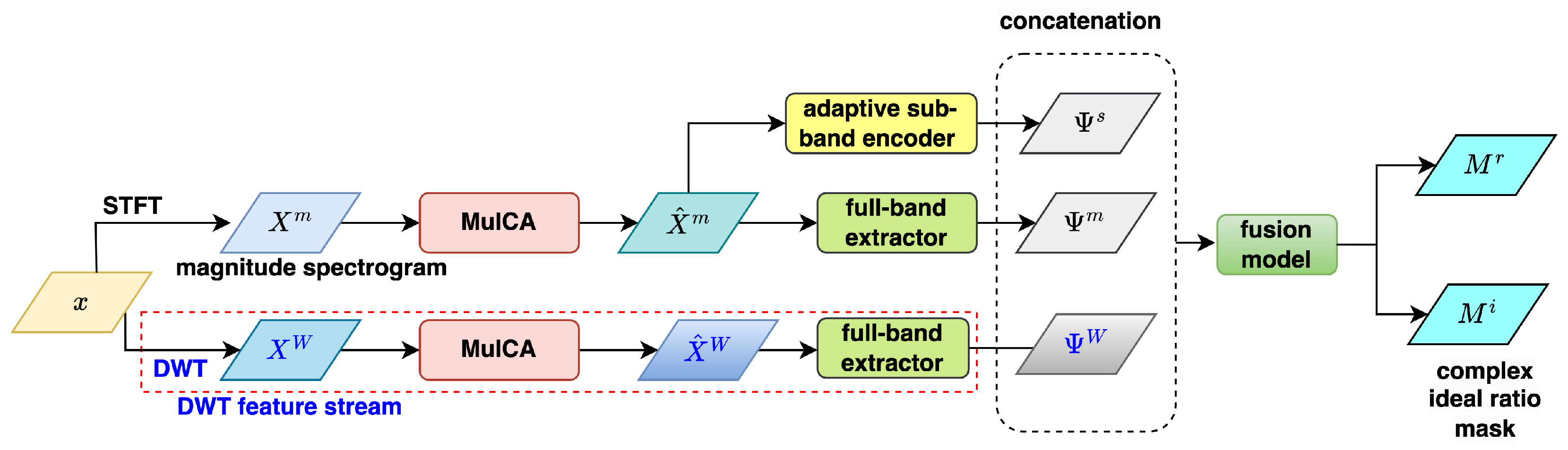
• Input stage: the input noisy speech signal x is transformed into the time-frequency domain using STFT, producing: magnitude spectrogram $X^m$, real-part spectrogram $X^r$, and imaginary-part spectrogram $X^i$.
• Full-band feature extraction: Following the FullSubNet+ architecture, A-FSN processes the input spectrograms $X^m$, $X^r$, and $X^i$ to extract global spectral information and long-distance cross-band dependencies. It includes a multi-scale time-sensitive channel attention (MulCA) module to assign weights to frequency bins. Furthermore, it utilizes temporal convolutional network (TCN) blocks to replace LSTMs for efficient modeling in the full-band extractor. In the following, we provide additional details about the MulCA module and the TCA blocks:
  • The MulCA module processes an input feature matrix (spectrogram here) through three parallel 1D depthwise convolutions with different kernel sizes along the time axis, extracting multi-scale features for each channel (frequency bin). These outputs undergo average pooling and ReLU activation, producing three time-scale features. A fully connected layer then combines these features into a single fusion feature, which is further processed by two additional fully connected layers to generate a weight vector representing the importance of each channel. Finally, this weight vector is applied to the input feature matrix via element-wise multiplication, resulting in a weighted feature matrix.
  • Each of the TCN blocks consists of a sequence of operations including input convolution, depthwise dilated convolution to capture long-range dependencies, and output convolution. The use of dilated convolutions allows TCNs to process sequences with varying dilation rates, effectively capturing both short-term and long-term temporal patterns.
• Adaptive sub-band processing: A-FSN incorporates an adaptive sub-band encoder module to process the unfolded magnitude spectrogram, drawing inspiration from the downsampling approach commonly used in time-domain speech enhancement techniques. The adaptive sub-band encoder is largely based on the encoding component of MANNER [47], a highly effective SE framework. The MANNER encoder is composed of a down-convolution layer, a residual Conformer (ResCon) block, and a multi-view attention (MA) block. By performing downsampling and feature encoding, and by stacking multiple encoder layers to form the sub-band encoder, compact and efficient sub-band features are extracted for further processing.
• Feature fusion: A fusion model combines the output of the full-band extractors (${\Psi }^m$, ${\Psi }^r$, and ${\Psi }^i$) with the adaptive sub-band encoder (${\Psi }^s$). The fusion model is built by stacking Conformer layers, similar to a TCN Block, with increasing dilation parameters. This design makes it easier to gather both long-term and short-term traits of speech. Notably, FullSubNet+ uses LSTM for the sub-band fusion model, but A-FSN replaces LSTM with Conformers to speed up implementation.
• cIRM prediction: The fused features are used to predict the complex ideal ratio mask (cIRM), $M^r$, and $M^i$, which suppress noise while preserving speech components in the time-frequency domain.
• Speech reconstruction: The enhanced complex spectrogram is converted back to the time domain using inverse STFT (iSTFT), producing the final clean speech waveform.

3. Presented Framework: DWT Features-Equipped A-FSN (WA-FSN)

In this study, we use the A-FSN as a base model and introduce some revisions to create a new SE framework. Specifically, we replace the complex-valued spectrogram input of A-FSN with discrete wavelet transform (DWT) feature sequences, while keeping most of the other components unchanged. The characteristics and potential advantages of the presented DWT features-equipped A-FSN (WA-FSN) are summarized as follows:

• The real and imaginary spectrogram inputs are replaced with frame-wise DWT feature sequences by simply adding a DWT operation module at the front end of A-FSN. Other modules, such as MulCA, the full-band extractor, the magnitude-based adaptive sub-band encoder, and the fusion model, remain unchanged. This localized revision allows us to focus specifically on the impact of DWT features on A-FSN.
• We employ one-level and two-level (extended) DWT to generate features, requiring, at most, six convolution operations. As a result, the additional computational load introduced by this approach is lightweight.
• DWT is a distortionless transformation that preserves all information from the input signal, similar to STFT’s real and imaginary spectrograms. Therefore, DWT features retain phase information, which is considered crucial for building an effective SE framework.
• DWT features can be viewed as time-domain features since they are generated by convolving input time-domain signals with predefined analysis filters. The resulting WA-FSN thus combines both time-domain and STFT-domain features to learn the cIRM, whereas the original A-FSN uses only STFT-domain features. Unlike typical learnable time-domain features in DNN-based SE models that require trainable convolution filters, DWT employs predefined filters for low-pass and high-pass operations. This makes DWT features easier to extract and more interpretable. Additionally, the importance of specific DWT sub-band features can be evaluated in WA-FSN by simply zeroing them out.

The flowchart of the newly proposed WA-FSN framework incorporating DWT features is illustrated in Figure 2. In comparison to the original A-FSN, shown in Figure 1, the only modification is the replacement of the real and imaginary spectrogram components ($X^r$ and $X^i$) with DWT features ($X^W$). WA-FSN retains the magnitude spectrogram as a feature source, along with most of the original components, such as the MulCA modules, full-band extractors, adaptive sub-band encoder, and the final fusion model. The DWT features are processed using the same modules as those for complex spectrograms in the original A-FSN. Specifically, these features pass through the MulCA module, which assigns importance weights to different frequency bins, followed by the full-band extractor, which utilizes TCN blocks. This processing pipeline is identical to how complex spectrograms are handled in A-FSN. As these components (MulCA and full-band extractor) are identical to those in the original A-FSN and have already been discussed in the previous section, we will not describe them again here. Instead, we will focus on explaining the procedures for generating various types of DWT features in the following two sub-sections.

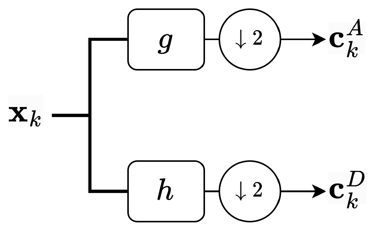
3.1. One-Level DWT Features

For an arbitrary data matrix $X\in {\mathbb{R}}^{L\times K}$, constructed by performing overlapped segmentation on an input time-domain signal x, we apply a one-level discrete wavelet transform (DWT) to each column ${\mathbf{x}}_k$ of X. Specifically, the frame signal ${\mathbf{x}}_k$ undergoes a one-level DWT, resulting in its factor-2 downsampled approximation (low-pass) and detail (high-pass) sub-band signals, denoted as ${\mathbf{c}}_k^A$ and ${\mathbf{c}}_k^D$, respectively. That is,

$$\begin{array}{cc}\hfill {\mathbf{c}}_k^A& =\sum _{n=0}^{L-1}{x}_k\left[n\right]·g[2m-n],(\mathrm{approximation}\mathrm{coefficients})\hfill \\ \hfill {\mathbf{c}}_k^D& =\sum _{n=0}^{L-1}{x}_k\left[n\right]·h[2m-n],(\mathrm{detail}\mathrm{coefficients})\hfill \end{array}$$

(1)

where $g\left[n\right]$ represents the low-pass filter coefficients, $h\left[n\right]$ denotes the high-pass filter coefficients derived from $g\left[n\right]$ via the quadrature mirror filter (QMF) relationship, $m=0,1,\dots ,\lfloor L/2\rfloor -1$ indicates the downsampled index, and $x_k\left[n\right]$ refers to the n-th sample of the frame vector ${\mathbf{x}}_k\in {\mathbb{R}}^L$.

The corresponding operations are depicted in Figure 3. Compared to the original vector ${\mathbf{x}}_k$, both ${\mathbf{c}}_k^A$ and ${\mathbf{c}}_k^D$ have reduced length and bandwidth, each being half that of ${\mathbf{x}}_k$. These sub-band signals are then organized into two feature matrices, $C^A$ and $C^D$, with dimensions ${\displaystyle \frac{L}{2}}\times K$, comprising the column vectors ${\mathbf{c}}_k^A$ and ${\mathbf{c}}_k^D$, respectively.

Using the resulting DWT sub-band matrices, $C^A$ and $C^D$, which represent the low-pass and high-pass components of the input time-domain data matrix X, we propose three arrangements to construct the DWT-based feature matrix (or matrices). This is done to investigate whether the emphasis on specific frequency ranges could impact the performance of WA-FSN.

The three proposed arrangements for constructing the DWT-based feature matrices are outlined as follows:

• Two individual branches
  In this arrangement, the two matrices $C^A$ and $C^D$ are vertically zero-padded to extend their size to $L\times K$, matching the dimensions of the original data matrix X. This is expressed as follows:

  $$X_A^W=[C^A;\mathbf{0}]\in {\mathbb{R}}^{L\times K},X_D^W=[\mathbf{0};C^D]\in {\mathbb{R}}^{L\times K},$$

  (2)

  where $\mathbf{0}$ is a zero matrix of size ${\displaystyle \frac{L}{2}}\times K$. The matrices $X_A^W$ and $X_D^W$ are then processed separately by the MulCA module and the full-band extractor to produce the final DWT feature matrices, ${\Psi }_A^W$ and ${\Psi }_D^W$. This setup mirrors the original A-FSN’s treatment of complex-valued spectrograms, where the real and imaginary components are handled as two independent feature branches.
• Single branch with concatenation
  Here, the matrices $C^A$ and $C^D$ are concatenated vertically to form a single DWT feature matrix:

  $$X^W=[C^A;C^D]=X_A^W+X_D^W\in {\mathbb{R}}^{L\times K},$$

  (3)

  which is then passed through the MulCA module and full-band extractor to generate the final DWT feature matrix, ${\Psi }^W$. This approach reduces the number of processing branches compared to the first arrangement, leading to a smaller model size and lower computational cost. Additionally, since $C^A$ and $C^D$ are combined into a single input, MulCA can simultaneously assign weights across both sub-bands, covering the entire frequency range and capturing mutual information between $C^A$ and $C^D$ more effectively.
• Single branch with dropping
  In this arrangement, one of the two branches from the first setup is discarded. Either $X_A^W$ or $X_D^W$, as defined in Equation (2), is used as the sole DWT feature input to undergo processing by the MulCA module and full-band extractor, resulting in a final DWT feature matrix of either ${\Psi }_A^W$ or ${\Psi }_D^W$. By adopting a single branch, this approach also reduces computational complexity and model size compared to the first arrangement. Additionally, it allows us to investigate which sub-band feature—approximation ($C^A$) or detail ($C^D$)—is more critical for enhancing WA-FSN’s performance in speech enhancement tasks.

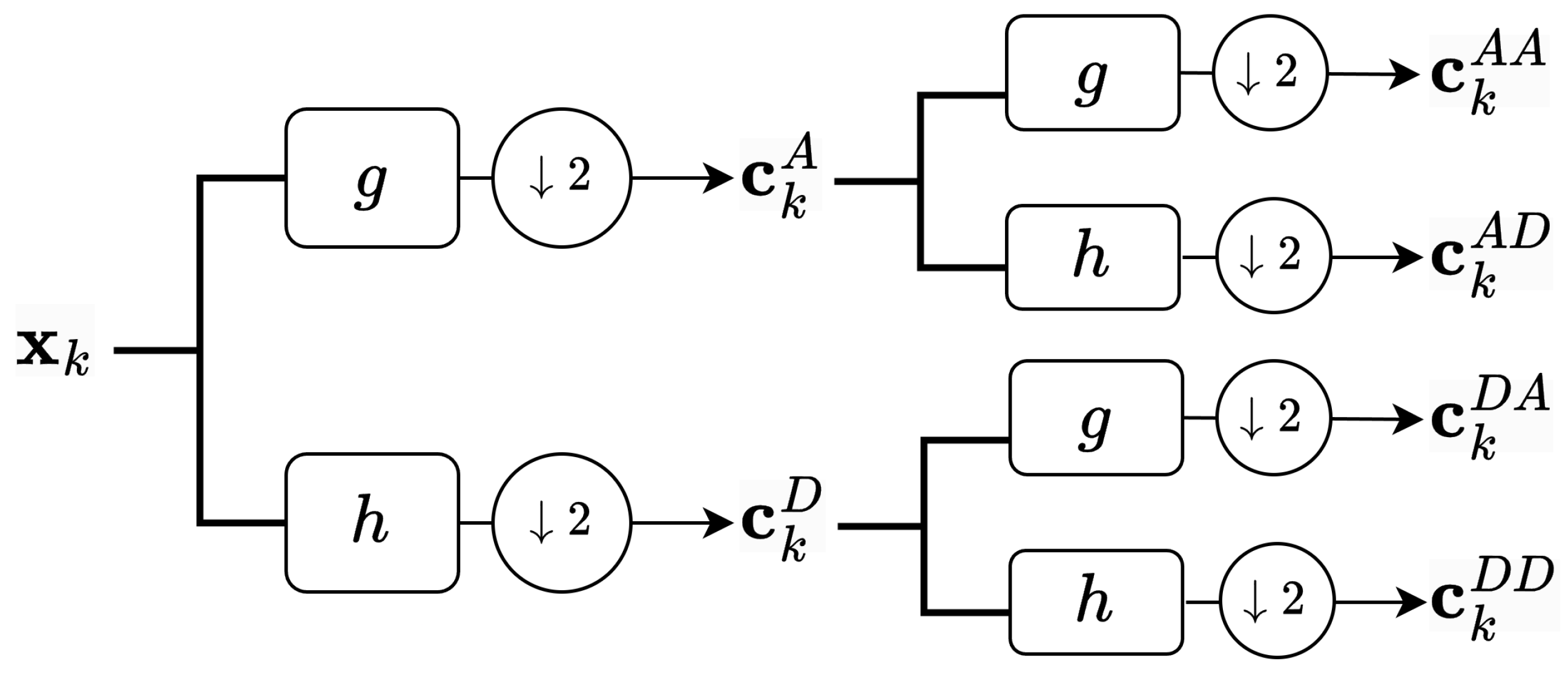
3.2. Two-Level DWT Features

A higher-level DWT can decompose the input signal into more sub-bands, focusing on the low-frequency (approximation) component and reducing the bandwidth of the sub-bands as the frequency decreases.

Here, we exploit an extension of two-level DWT, known as two-level wavelet packet decomposition (WPD) [43], to produce multiple sub-bands. This method applies low-pass/high-pass filtering and downsampling to both the approximation and detail components generated by the one-level DWT, resulting in four sub-band signals with approximately equal bandwidths. Compared to one-level DWT outputs, two-level (extended) DWT outputs have half the bandwidth. This allows us to explore whether finer frequency resolution from two-level DWT signals improves WA-FSN performance and to assess the relative importance of these sub-bands.

Using the notations from the previous subsection, each frame signal ${\mathbf{x}}_k$ undergoes a two-level DWT, producing four sub-band signals: ${\mathbf{c}}_k^{DD}$, ${\mathbf{c}}_k^{DA}$, ${\mathbf{c}}_k^{AD}$, and ${\mathbf{c}}_k^{AA}$. The corresponding flowchart is shown in Figure 4. These sub-band signals are organized into four feature matrices, $C^{DD}$, $C^{DA}$, $C^{AD}$, and $C^{AA}$, each with dimensions ${\displaystyle \frac{L}{4}}\times K$, where ${\mathbf{c}}_k^{DD}$, ${\mathbf{c}}_k^{DA}$, ${\mathbf{c}}_k^{AD}$, and ${\mathbf{c}}_k^{AA}$ form the columns of their respective matrices. These two-level DWT sub-band matrices are then merged into a single branch of DWT features, which is passed through the MulCA module and full-band extractor to produce the final feature matrix ${\Psi }^W$. Before merging and processing, we consider two arrangements for these sub-band matrices:

• Concatenation of all sub-bands
  All four sub-band feature matrices are concatenated vertically to form a single DWT feature matrix:

  $$X^W=[C^{DD};C^{DA};C^{AD};C^{AA}]\in {\mathbb{R}}^{L\times K}.$$

  (4)
• Concatenation of adjacent sub-bands
  To evaluate the relative importance of specific sub-bands, we selectively concatenate two or three adjacent sub-band matrices vertically to form a single DWT feature matrix. The possible configurations are as follows:

  (a)

  The lowest three sub-bands:

  $$X^W=[C^{DA};C^{AD};C^{AA}],$$

  (5)

  (b)

  The highest three sub-bands:

  $$X^W=[C^{DD};C^{DA};C^{AD}],$$

  (6)

  (c)

  The lowest two sub-bands:

  $$X^W=[C^{AD};C^{AA}],$$

  (7)

  (d)

  The highest two sub-bands:

  $$X^W=[C^{DD};C^{DA}].$$

  (8)

Furthermore, we employ a zero-padding technique to augment the features by filling in insufficient parts with zeros. This approach is similar to the method used for one-level DWT features. By using zero-padding, we maintain consistent dimensions for each sub-band after DWT decomposition, which facilitates more effective feature extraction and learning by the model.

To show that adding DWT features in WA-FSN does not significantly increase computational complexity compared to A-FSN (which uses DFT/STFT), we compare DWT and DFT in

Table 1. Comparison between DFT and DWT for an input signal of length N.

Transform	FLOPs	Runtime Complexity
DFT (direct computation)	$O\left(N^2\right)$	$O\left(N^2\right)$
DFT (FFT algorithm)	$O(NlogN)$	$O(NlogN)$
One-level DWT (filter length M)	$O\left(MN\right)$	$O\left(N\right)$
Two-level DWT (filter length M)	$O\left(MN\right)$	$O\left(N\right)$

. The comparison reveals DWT adds minimal computational overhead, maintaining WA-FSN’s efficiency. FLOPs (Floating Point Operations) measure arithmetic operations independently of hardware, while runtime is the actual execution time, varying with implementation. Higher FLOPs often correlate with longer runtimes, but not always linearly due to factors like parallelization.

From this table, we can make some key observations:

• The DWT maintains a computational efficiency advantage over DFT/FFT for large N while providing more detailed frequency analysis. This makes it particularly useful for applications requiring multi-resolution analysis.
• The two-level DWT still requires $O\left(MN\right)$ floating-point operations because:

  –

  First level processes N samples: $O(MN/2)$

  –

  Second level processes N/2 samples: $O(MN/4)$

  –

  Total: $O(MN/2+MN/4)=O(3MN/4)=O\left(MN\right)$

• Runtime complexity for both one-level and two-level DWT remains $O\left(N\right)$, as the algorithm still processes the signal linearly.
• Two-level DWT provides finer frequency resolution in lower frequency bands without significantly increasing computational complexity compared to one-level DWT.
• Two-level DWT requires slightly more memory to store intermediate results, but the order of magnitude remains the same as one-level DWT.

4. Experimental Setup

Our evaluation utilizes the VoiceBank-DEMAND task, combining the VoiceBank speech dataset [48] with noise from the DEMAND database [49]. The training set comprises 11,572 utterances from 28 speakers, while the test set contains 824 utterances from 2 speakers. Training data are corrupted with ten DEMAND noise types at 0, 5, 10, and 15 dB SNRs, whereas test data use five DEMAND noises at 2.5, 7.5, 12.5, and 17.5 dB SNRs. Approximately 200 utterances are set aside for validation.

For feature transformation, the input signal is segmented into frames using a Hanning window with a length of 32 ms (512 points) and a shift of 16 ms (256 points). Each frame is converted into STFT spectrograms using a 512-point DFT, and various DWT features are generated as described in the proposed method. The db2 wavelet function is employed for DWT. This four-point wavelet enables simple convolution filtering and is widely used for its effective feature isolation, as noted in [50].

On the model side, the MulCA module uses 257 channels with parallel 1D depthwise convolutions having kernel sizes of 3, 5, and 10. Each full-band extractor employs two groups of TCN blocks, with each group consisting of four TCN blocks featuring a kernel size of 3 and dilation rates of 1, 2, 5, and 9. The sub-band encoder starts with 64 initial frequency bins, resulting in 129 adjacent bins for sub-band features. It includes two layers with down-convolutions using a kernel size of (4, 2) and a stride of (8, 4). The fusion model stacks three Conformer layers with dilation parameters set to 1, 2, and 5, expanding features four times with a kernel size of 31. The training follows the original A-FSN setup, using the Adam optimizer with a learning rate of 0.001, an input sequence length of 192 frames, and 2 look-ahead frames for processing each frame.

To evaluate the effectiveness of speech enhancement (SE) approaches, we employ three objective indicators:

• Perceptual estimation of speech quality (PESQ) [51]: This metric assesses the perceived speech quality, ranging from −0.5 to 4.5, with higher scores indicating better quality. PESQ objectively quantifies speech quality by comparing processed speech to the original clean speech. The computation involves time alignment, level alignment, time-frequency mapping, frequency warping, and compressive loudness scaling.
• Short-time objective intelligibility (STOI) [52]: This metric evaluates the objective intelligibility of short-time, time-frequency areas in an utterance using the discrete-time Fourier transform. STOI scores range from 0 to 1, with higher values indicating better intelligibility. The calculation involves applying STFT to processed and clean signals, conducting one-third octave band analysis, normalizing and clipping energy, and computing linear correlation coefficients between estimated and original signals.
• Scale-invariant signal-to-noise ratio (SI-SNR) [53]: This metric measures artifact distortion between processed and clean speech. It is calculated as follows:

  $$\mathrm{SI}\text{-}\mathrm{SNR}=10{log}_{10}\left({\displaystyle \frac{\parallel {\mathbf{s}}_{target}{\parallel }^2}{\parallel {\mathbf{e}}_{noise}{\parallel }^2}}\right),$$

  (9)

  where

  $${\mathbf{s}}_{target}={\displaystyle \frac{\langle \widehat{\mathbf{s}},\mathbf{s}\rangle \mathbf{s}}{{\parallel \mathbf{s}\parallel }^2}},$$

  (10)

  $${\mathbf{e}}_{noise}=\widehat{\mathbf{s}}-{\mathbf{s}}_{target},$$

  (11)

  with $\langle \widehat{\mathbf{s}},\mathbf{s}\rangle$ being the inner product of $\widehat{\mathbf{s}}$ and $\mathbf{s}$.

It is worth noting that PESQ, STOI, and SI-SNR are widely used metrics in the speech enhancement community, facilitating standardized comparisons across various studies and methodologies. By employing these metrics, we can comprehensively evaluate our proposed WA-FSN model, addressing key aspects such as speech quality, intelligibility, and noise reduction, which are crucial for real-world applications. This approach ensures a balanced assessment of the model’s performance, aligning with the needs of practical speech enhancement tasks.

5. Experimental Results and Discussions

5.1. Selection of Sub-Band Fusion Model Structure

One of the particularities of A-FSN is to use Conformer to substitute LSTM while developing its fusion model. This can help decrease the size of the model and speed up the calculation. However, the results of our preliminary examination show that Conformer does not always perform better than LSTM in some of the SE metrics for both A-FSN and WA-FSN.

Table 2. The results of A-FSN and WA-FSN with different structures of its fusion model: Conformer and LSTM.

Feature	A-FSN		WA-FSN
Fusion Model	Conformer	LSTM	Conformer	LSTM
PESQ	2.8051	2.7885	2.7586	2.7926
STOI	0.9406	0.9394	0.9405	0.9422
SI-SNR	17.65	18.02	18.02	18.55

presents these findings, where the LSTM-based fusion model consists of two stacked unidirectional LSTM layers each with 384 hidden units, and WA-FSN uses one-level DWT features in a single branch with concatenation. From this table, we have the following observations:

• As with the original A-FSN (using complex spectrograms), selecting a Conformer other than LSTM as the fusion model can improve PESQ and STOI scores moderately while degrading SI-SNR. This indicates that using Conformer in A-FSN is primarily intended to reduce the model’s complexity, as opposed to enhancing its SE behavior.
• When Conformer is used as the fusion model, the presented WA-FSN (with DWT features) provides worse PESQ, comparable STOI, and higher SI-SNR than the original A-FSN. However, replacing Conformer with LSTM for the fusion model in the WA-FSN significantly promotes all of the three metrics. Furthermore, WA-FSN with LSTM outperforms A-FSN with Conformer in STOI and SI-SNR scores apparently.
• Conformer excels at handling complex spectrograms, while LSTM is proficient in dealing with certain parts of wavelet features. Our interpretation is that Conformer, in order to reduce computational complexity, tends to extract fixed and partial information. However, for wavelet features, it is more suitable to retain the entire feature information. Therefore, the computationally more complex LSTM is better suited for handling wavelet features.

Based on these initial results, LSTM seems to be a more appropriate fusion model for the presented WA-FSN. Hence, unless otherwise mentioned, LSTM is used as the fusion model for A-FSN and all forms of WA-FSN in the following evaluation experiments.

5.2. Results for WA-FSN with One-Level DWT Features

Table 3. The SE results for the unprocessed baseline, A-FSN, and WA-FSN variants with one-level DWT features.

Methods			PESQ	STOI	SI-SNR
unprocessed			1.9700	0.9210	8.45
A-FSN (LSTM)			2.7885	0.9394	18.02
WA-FSN	two branches		2.8184	0.9432	17.86
	one branch	concatenation	2.7926	0.9422	18.55
		$C^A$	2.8875	0.9425	17.97
		$C^D$	2.8886	0.9424	17.99

shows the PESQ, STOI, and SI-SNR results for WA-FSN with one-level DWT features, which might be one branch or two branches as described in Section 3.1. From this table, we have the following observations:

• All versions of WA-FSN with one-level DWT outperform A-FSN in the two SE metrics, PESQ and STOI, confirming that the DWT features can benefit A-FSN by providing superior or comparable SE outputs. However, A-FSN gives better SI-SNR scores than most WA-FSN variants (except for the concatenation case).
• The two-branch WA-FSN, which processes the approximation and detail parts separately ($C^A$ and $C^D$) and has the same model structure as A-FSN, outperforms A-FSN moderately in PESQ but substantially in STOI. This result suggests that when it comes to two-branch processing, it is more prudent to select the DWT-wise approximation and detail portions than the real and imaginary spectrograms.
• Regarding the three cases that deal with DWT features using a single branch, the STOI results are very similar, implying that STOI has less relevance to the selection of DWT-sub-bands. However, using either $C^A$ or $C^D$ alone results in significantly higher PESQ scores than using both in concatenation. One possible explanation is that the one-branch model is less effective at dealing with the full-band information (in the concatenation of $C^A$ and $C^D$) to calibrate the speech signal more precisely. Contrarily, the concatenation case outperforms the individual half-band cases ($C^A$ and $C^D$) in SI-SNR, likely due to the fact that the concatenation case can provide superior noise reduction to the entire bands. However, this explanation requires further validation.

5.3. Experiments on WA-FSN with Two-Level DWT Features

In

Table 4. The SE results for the unprocessed baseline, original A-FSN, and WA-FSN variant with two-level DWT features.

Methods		PESQ	STOI	SI-SNR
unprocessed		1.9700	0.9210	8.45
A-FSN (LSTM)		2.7885	0.9394	18.02
WA-FSN with one-level DWT features	concatenation	2.7926	0.9422	18.55
WA-FSN with two-level DWT features	all four sub-bands	2.8676	0.9432	18.25
	the lowest three sub-bands	2.8937	0.9430	18.24
	the highest three sub-bands	2.8277	0.9437	18.27
	the lowest two sub-bands	2.8782	0.9423	18.34
	the highest two sub-bands	2.7912	0.9424	18.83

, we present the results of three SE metrics for WA-FSN using two-level DWT features. In pursuit of simplicity, we only use one branch to process the two-level DWT sub-band outputs. Included for comparison purposes are the results of WA-FSN using one-level DWT with concatenation (one branch). From this table, the following observations can be made:

• When two-level DWT is utilized, each of the resulting WA-FSN variants outperforms the original A-FSN in terms of PESQ, STOI, and SI-SNR, apparently indicating a superior performance in the SE task.
• Using either of the lowest three sub-bands or the lowest two sub-bands can further improve PESQ (from $2.8676$ to $2.8937$ and $2.8782$), respectively, compared to the full-band case. However, the cases with the highest three sub-bands and the highest two sub-bands attain lower PESQ scores ($2.8277$ and $2.7912$, respectively), indicating that the lower sub-bands contribute more to PESQ than the higher sub-bands.
• In terms of STOI, the choice of sub-bands does not result in a significant difference, but selecting three sub-bands seems preferable to selecting two ($0.9437$ and $0.9423$ vs. $0.9423$ and $0.9424$). In contrast, cases with two sub-bands have a higher SI-SNR than those with three sub-bands. Notably, the selection of the two highest sub-bands achieves an SI-SNR value ($18.83$ dB) that is significantly better than all other selections.

Based on these experimental findings, there is no single selection of two-level DWT-wise sub-bands that can simultaneously obtain optimal PESQ, STOI, and SI-SNR scores. First, even if the neighboring sub-bands of the two-level DWT are selected at random, it is unlikely that the SE performance will be unusually poor. The selection of sub-bands can also be influenced by the SE metric that we wish to emphasize. For instance, if PESQ is of particular concern, we can employ the three lowest sub-band cases, whereas the option of the highest sub-band case may be favored if we are primarily concerned with promoting the SI-SNR score.

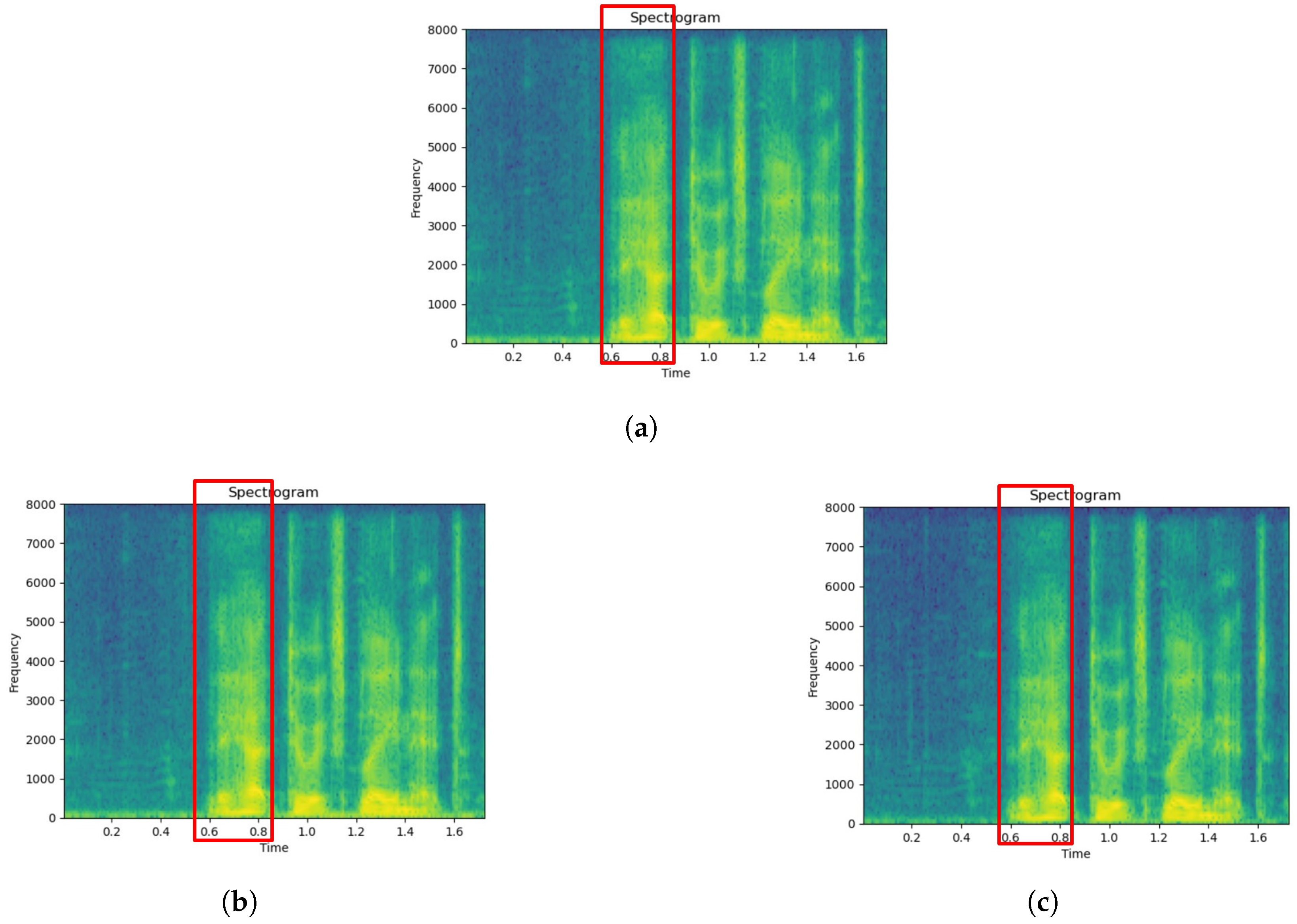
5.4. Spectrogram Demonstration for SE Methods

In addition to the objective perceptual metrics, here we use the magnitude spectrograms of a sample utterance in different situations to examine the denoising performance of WA-FSN. For simplicity, here we just test the two-level WA-FSN variants, as they provide better SE metric scores. These magnitude spectrogram plots are shown in Figure 5, Figure 6 and Figure 7, from which we have some findings:

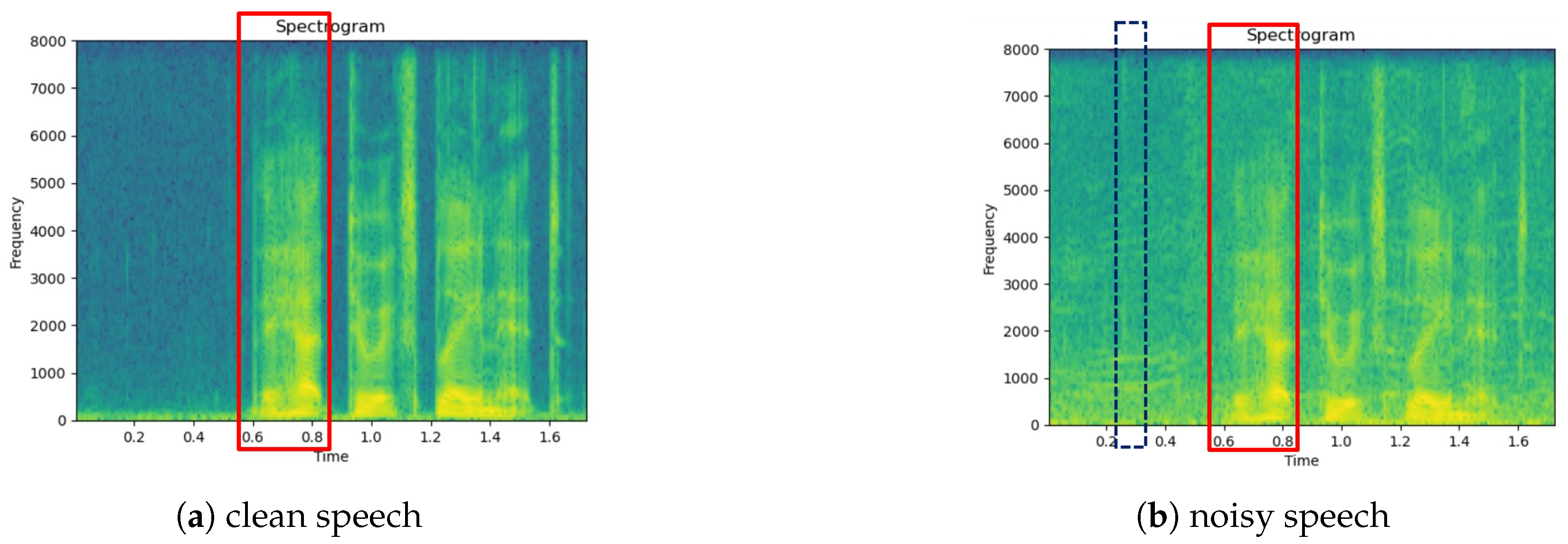
• Comparing Figure 5a and b, which correspond to a clean utterance and its unprocessed noisy counterpart, respectively, we can observe that noise significantly distorts the entire time range of the utterance, causing the formant and harmonic structure of the speech component to almost completely disappear.
• Compared to the original noisy utterance, the enhanced versions produced by the WA-FSN variants effectively reduce noise distortion and emphasize the distinction between speech and non-speech segments. For example, the area between 0.6 and 0.8 s, highlighted by a red box in Figure 6 (using at least three sub-bands) and Figure 7 (using two sub-bands), shows a greater variation in energy compared to the unprocessed noisy case in Figure 5b.
• Figure 7a,b, which utilize two sub-bands in WA-FSN, exhibit slightly more residual noise (notably around 2.5 s, marked by a blue box) compared to Figure 6a–c, which employ at least three sub-bands. This suggests that using more sub-bands can enhance noise reduction. However, the difference is not entirely evident, likely because the full-band magnitude spectrogram provides comprehensive information. Additionally, the distinction between Figure 7a (using the lowest two sub-bands) and Figure 7b (using the highest two sub-bands) is not clear, possibly due to the similar speech enhancement metrics shown in Table 4.

6. Conclusions

This study explores deep learning-based speech enhancement methods by integrating discrete wavelet transform (DWT) features into the adaptive FullSubNet (A-FSN) framework, creating the WA-FSN model. WA-FSN uses one-level or two-level DWT features alongside STFT magnitude spectrograms to predict the complex ideal ratio mask (cIRM) for noise reduction. Experiments on the VoiceBank-DEMAND dataset show that DWT features complement STFT features, improving performance in PESQ and SI-SNR metrics. DWT features are a viable alternative to STFT complex spectrograms due to their faster generation and effectiveness in enhancing speech enhancement outcomes.

The proposed WA-FSN framework offers several real-world benefits. Its improvements in SI-SNR enhance noise suppression, benefiting hearing aid users in crowded spaces. The reduced computational complexity allows deployment on resource-constrained devices like smart speakers and IoT endpoints. The decoupled DWT/STFT features enable independent optimization for ASR (prioritizing PESQ) and communication systems (emphasizing STOI). Additionally, WA-FSN’s modular architecture provides diagnostic flexibility for audio forensics by allowing selective sub-band suppression. These advantages highlight WA-FSN’s potential to improve speech communication in challenging environments.

Despite the advantages shown above, the proposed WA-FSN method has several limitations. It requires manual optimization of DWT sub-band combinations for different SE metrics, as no single configuration optimizes all metrics simultaneously, adding deployment complexity. The use of predefined db2 wavelets instead of learnable filters may limit adaptability to diverse noise types compared to trainable encoders.

For future research, several avenues can be explored to further optimize and extend the WA-FSN approach:

• Investigate the impact of different wavelet functions: Examining wavelet functions such as db4 and db8 could help identify those that better capture specific noise patterns or speech characteristics, potentially improving WA-FSN performance.
• Develop advanced fusion strategies: Creating more sophisticated methods for combining features from DWT and STFT could enhance effectiveness. This might include using learning-based techniques to dynamically adjust the importance of each feature type depending on the characteristics of the input signal.
• Examine the transferability of DWT features: Research how DWT features can be applied to other speech enhancement frameworks, such as DEMUCS [54] and MANNER [47]. This could provide insights into the generalizability of DWT-based features across different architectures.
• Optimize WA-FSN for real-time deployment: To enable real-time application, it will be important to reduce computational complexity while maintaining performance. This could involve techniques such as model pruning or knowledge distillation.

By pursuing these research directions, future studies can build upon the WA-FSN framework to achieve even better speech enhancement outcomes in a variety of acoustic environments.

References

- Boll, S.F. Suppression of acoustic noise in speech using spectral subtraction. IEEE Trans. Acoust. Speech Signal Process. 1979, 27, 113–120. [Google Scholar] [CrossRef]
- Scalart, P.; Filho, J.V. Speech enhancement based on a priori signal to noise estimation. In Proceedings of the International Conference on Acoustics, Speech and Signal Processing (ICASSP), Atlanta, GA, USA, 7–10 May 1996. [Google Scholar]
- Gauvain, J.L.; Lee, C.H. Maximum a posteriori estimation for multivariate Gaussian mixture observations of Markov chains. IEEE Trans. Speech Audio Process. 1994, 2, 291–298. [Google Scholar]
- Ephraim, Y.; Malah, D. Speech enhancement using a minimum mean-square error log-spectral amplitude estimator. IEEE Trans. Acoust. Speech Signal Process. 1985, 33, 443–445. [Google Scholar]
- Wu, J.; Huo, Q. An environment-compensated minimum classification error training approach based on stochastic vector mapping. IEEE Trans. Audio Speech Lang Process. 2006, 14, 2147–2155. [Google Scholar]
- Xu, Y.; Du, J.; Dai, L.; Lee, C. A regression approach to speech enhancement based on deep neural networks. IEEE/ACM Trans. Audio Speech, Lang. Process. 2015, 23, 7–19. [Google Scholar]
- Zhao, Y.; Wang, D.; Merks, I.; Zhang, T. DNN-based enhancement of noisy and reverberant speech. In Proceedings of the International Conference on Acoustics, Speech and Signal Processing (ICASSP), Shanghai, China, 20–25 March 2016. [Google Scholar]
- Wang, D. Deep learning reinvents the hearing aid. Inst. Electr. Electron. Eng. (IEEE) Spectr. 2017, 54, 32–37. [Google Scholar]
- Chen, J.; Wang, Y.; Yoho, S.E.; Wang, D.; Healy, E.W. Large-scale training to increase speech intelligibility for hearing-impaired listeners in novel noises. J. Acoust. Soc. Am. 2016, 139, 2604–2612. [Google Scholar]
- Karjol, P.; Kumar, M.A.; Ghosh, P.K. Speech enhancement using multiple deep neural networks. In Proceedings of the International Conference on Acoustics, Speech and Signal Processing (ICASSP), Shanghai, China, 20–25 March 2016. [Google Scholar]
- Kounovsky, T.; Malek, J. Single channel speech enhancement using convolutional neural network. In Proceedings of the ECMSM, Donostia-San Sebastian, Spain, 24–26 May 2017. [Google Scholar]
- Chakrabarty, S.; Wang, D.; Habets, E.A.P. Time-frequency masking based online speech enhancement with multi-channel data Using convolutional neural Networks. In Proceedings of the IWAENC, Tokyo, Japan, 17–20 September 2018. [Google Scholar]
- Luo, Y.; Mesgarani, N. Conv-tasnet: Surpassing ideal time–frequency magnitude masking for speech separation. IEEE/ACM Trans. Audio Speech Lang. Process. 2019, 27, 1256–1266. [Google Scholar] [CrossRef]
- Fu, S.; Tsao, Y.; Lu, X.; Kawai, H. Raw waveform-based speech enhancement by fully convolutional networks. In Proceedings of the APSIPA ASC, Kuala Lumpur, Malaysia, 12–15 December 2017. [Google Scholar]
- Kiranyaz, S.; Ince, T.; Abdeljaber, O.; Avci, O.; Gabbouj, M. 1-D convolutional neural networks for signal processing applications. In Proceedings of the ICASSP, Brighton, UK, 12–17 May 2019. [Google Scholar]
- Wang, D.; Rong, X.; Sun, S.; Hu, Y.; Zhu, C.; Lu, J. Adaptive Convolution for CNN-based Speech Enhancement Models. arXiv 2025, arXiv:2502.14224. [Google Scholar]
- Sach, M.; Franzen, J.; Defraene, B.; Fluyt, K.; Strake, M.; Tirry, W.; Fingscheidt, T. EffCRN: An Efficient Convolutional Recurrent Network for High-Performance Speech Enhancement. In Proceedings of the Interspeech, Dublin, Ireland, 20–24 August 2023; pp. 656–660. [Google Scholar]
- Yin, H.; Bai, J.; Wang, M.; Huang, S.; Jia, Y.; Chen, J. Convolutional Recurrent Neural Network with Attention for 3D Speech Enhancement. arXiv 2023, arXiv:2306.04987. [Google Scholar]
- Jannu, C.; Vanambathina, S.D. Convolutional Transformer based Local and Global Feature Learning for Speech Enhancement. Int. J. Adv. Comput. Sci. Appl. 2023, 14, 731–743. [Google Scholar] [CrossRef]
- Chung, J.; Gulcehre, C.; Cho, K.; Bengio, Y. Empirical evaluation of gated recurrent neural networks on sequence modeling. arXiv 2014, arXiv:1412.3555. [Google Scholar]
- Sun, L.; Du, J.; Dai, L.; Lee, C. Multiple-target deep learning for LSTM-RNN based speech enhancement. In Proceedings of the Hands-Free Speech Communication and Microphone Arrays (HSCMA), San Francisco, CA, USA, 1–3 March 2017. [Google Scholar]
- Cheng, L.; Pandey, A.; Xu, B.; Delbruck, T.; Liu, S.C. Dynamic Gated Recurrent Neural Network for Compute-efficient Speech Enhancement. arXiv 2024, arXiv:2408.12425. [Google Scholar]
- Botinhao, C.V.; Wang, X.; Takaki, S.; Yamagishi, J. Speech Enhancement for a Noise-Robust Text-to-Speech Synthesis System Using Deep Recurrent Neural Networks. In Proceedings of the Interspeech 2016, San Francisco, CA, USA, 8–12 September 2016. [Google Scholar]
- Goodfellow, I.; Pouget-Abadie, J.; Mirza, M.; Xu, B.; Warde-Farley, D.; Ozair, S.; Courville, A.; Bengio, Y. Generative adversarial networks. Commun. ACM 2020, 63, 139–144. [Google Scholar] [CrossRef]
- Andreev, P. Generative Models for Speech Enhancement. Ph.D. Thesis, HSE University, Moscow, Russia, 2024. Available online: https://www.hse.ru/data/2024/10/04/1888260947/%D0%90%D0%BD%D0%B4%D1%80%D0%B5%D0%B5%D0%B2_summary.pdf (accessed on 27 March 2025).
- Shetu, S.S.; Habets, E.A.; Brendel, A. GAN-Based Speech Enhancement for Low SNR Using Latent Feature Conditioning. arXiv 2023, arXiv:2410.13599. [Google Scholar]
- Strauss, M. SEFGAN: Harvesting the Power of Normalizing Flows and GANs for Efficient High-Quality Speech Enhancement. arXiv 2023, arXiv:2312.01744. [Google Scholar]
- Chen, J.; Mao, Q.; Liu, D. Dual-Path Transformer Network: Direct Context-Aware Modeling for End-to-End Monaural Speech Separation. arXiv 2020, arXiv:2007.13975. [Google Scholar]
- Zhang, S.; Chadwick, M.; Ramos, A.G.; Parcollet, T.; van Dalen, R.; Bhattacharya, S. Real-Time Personalised Speech Enhancement Transformers with Cross-Attention. In Proceedings of the Interspeech 2023, Dublin, Ireland, 20–24 August 2023. [Google Scholar]
- Chao, F.A.; Hung, J.W.; Chen, B. Multi-view Attention-based Speech Enhancement Model for Noise-robust Automatic Speech Recognition. In Proceedings of the 32nd Conference on Computational Linguistics and Speech Processing (ROCLING 2020), Taipei, Taiwan, 24–26 September 2020. [Google Scholar]
- Bai, J.; Li, H.; Zhang, X.; Chen, F. Attention-Based Beamformer For Multi-Channel Speech Enhancement. arXiv 2024, arXiv:2409.06456. [Google Scholar]
- Wang, Y.; Narayanan, A.; Wang, D. On training targets for supervised speech separation. IEEE/ACM Trans. Audio Speech Lang. Process. 2014, 22, 1849–1858. [Google Scholar] [CrossRef]
- Wang, D.; Chen, J. Supervised speech separation based on deep learning: An overview. IEEE/ACM Trans. Audio Speech Lang. Process. 2018, 26, 1702–1726. [Google Scholar]
- Roman, N.; Woodruff, J. Ideal binary masking in reverberation. In Proceedings of the 20th European Signal Processing Conference (EUSIPCO), Bucharest, Romania, 27–31 August 2012; pp. 629–633. [Google Scholar]
- Narayanan, A.; Wang, D. Ideal ratio mask estimation using deep neural networks for robust speech recognition. In Proceedings of the 2013 IEEE International Conference on Acoustics, Speech and Signal Processing (ICASSP), Vancouver, BC, Canada, 26–31 May 2013; pp. 7092–7096. [Google Scholar] [CrossRef]
- Williamson, D.S.; Wang, Y.; Wang, D. Complex ratio masking for monaural speech separation. IEEE/ACM Trans. Audio Speech Lang. Process. 2016, 24, 483–492. [Google Scholar] [CrossRef] [PubMed]
- Erdogan, H.; Hershey, J.R.; Watanabe, S.; Roux, J.L. Phase-sensitive and recognition-boosted speech separation using deep recurrent neural networks. In Proceedings of the International Conference on Acoustics, Speech and Signal Processing (ICASSP), Brisbane, Australia, 19–24 April 2015. [Google Scholar]
- Hao, X.; Su, X.; Horaud, R.; Li, X. Fullsubnet: A full-band and sub-band fusion model for real-time single-channel speech enhancement. In Proceedings of the ICASSP 2021—2021 IEEE International Conference on Acoustics, Speech and Signal Processing (ICASSP), Toronto, ON, Canada, 6–11 June 2021. [Google Scholar]
- Chen, J.; Wang, Z.; Tuo, D.; Wu, Z.; Kang, S.; Meng, H. Fullsubnet+: Channel attention fullsubnet with complex spectrograms for speech enhancement. In Proceedings of the ICASSP 2022—2022 IEEE International Conference on Acoustics, Speech and Signal Processing (ICASSP), Virtual, 7–13 May 2022. [Google Scholar]
- Tsao, Y.S.; Ho, K.H.; Hung, J.W.; Chen, B. Adaptive-FSN: Integrating Full-Band Extraction and Adaptive Sub-Band Encoding for Monaural Speech Enhancement. In Proceedings of the 2023 IEEE Spoken Language Technology Workshop (SLT), Doha, Qatar, 9–12 January 2023. [Google Scholar]
- Gulati, A.; Qin, J.; Chiu, C.C.; Parmar, N.; Zhang, Y.; Yu, J.; Han, W.; Wang, S.; Zhang, Z.; Wu, Y.; et al. Conformer: Convolution-augmented transformer for speech recognition. arXiv 2020, arXiv:2005.08100. [Google Scholar]
- Mallat, S. A Wavelet Tour of Signal Processing, 2nd ed.; Academic: San Diego, CA, USA, 1999. [Google Scholar]
- Mitra, S.K. Digital Signal Processing, a Computer-Based Approach, 4th ed.; Wcb/McGraw-Hill: New York, NY, USA, 2010. [Google Scholar]
- Vani, H.Y.; Anusuya, M.A. Hilbert Huang transform based speech recognition. In Proceedings of the 2016 Second International Conference on Cognitive Computing and Information Processing (CCIP), Mysuru, India, 2–13 August 2016; pp. 1–6. [Google Scholar] [CrossRef]
- Ravanelli, M.; Bengio, Y. Speech and speaker recognition from raw waveform with sincnet. In Proceedings of the 2018 IEEE Spoken Language Technology Workshop (SLT), Athens, Greece, 18–21 December 2018. [Google Scholar]
- Wu, P.-C.; Li, P.-F.; Wu, Z.-T.; Hung, J.-W. The Study of Improving the Adaptive FullSubNet+ Speech Enhancement Framework with Selective Wavelet Packet Decomposition Sub-Band Features. In Proceedings of the 2023 9th International Conference on Applied System Innovation (ICASI), Chiba, Japan, 21–25 April 2023. [Google Scholar]
- Park, H.J.; Kang, B.H.; Shin, W.; Kim, J.S.; Han, S.W. MANNER: Multi-View Attention Network For Noise Erasure. In Proceedings of the ICASSP 2022—2022 IEEE International Conference on Acoustics, Speech and Signal Processing (ICASSP), Virtual, 7–13 May 2022; pp. 7842–7846. [Google Scholar] [CrossRef]
- Veaux, C.; Yamagishi, J.; King, S. The voice bank corpus: Design, collection and data analysis of a large regional accent speech database. In Proceedings of the Conference on Asian Spoken Language Research and Evaluation (OCOCOSDA/CASLRE), Gurgaon, India, 25–27 November 2013. [Google Scholar]
- Thiemann, J.; Ito, N.; Vincent, E. Demand: A collection of multi-channel recordings of acoustic noise in diverse environments. In Proceedings of the Meetings Acoust, Montreal, QC, Canada, 2–7 June 2013. [Google Scholar]
- Daubechies, I. Orthonormal bases of compactly supported wavelets. Commun. Pure Appl. Math. 1988, 41, 909–996. [Google Scholar]
- Union, I.T. Perceptual Evaluation of Speech Quality (pesq): An Objective Method for End-to-End Speech Quality Assessment of Narrow-Band Telephone Networks and Speech Codecs. ITU-T Recommendation, P. 862. 2001. Available online: https://cir.nii.ac.jp/crid/1574231874837257984 (accessed on 27 March 2025).
- Taal, C.H.; Hendriks, R.C.; Heusdens, R.; Jensen, J. A short-time objective intelligibility measure for time-frequency weighted noisy speech. In Proceedings of the 2010 IEEE International Conference on Acoustics, Speech and Signal Processing, Dallas, TX, USA, 14–19 March 2010. [Google Scholar]
- Isik, Y.; Roux, J.L.; Chen, Z.; Watanabe, S.; Hershey, J.R. Single-channel multi-speaker separation using deep clustering. In Proceedings of the Interspeech 2016, San Francisco, CA, USA, 8–12 September 2016. [Google Scholar]
- Defossez, A.; Synnaeve, G.; Adi, Y. Real time speech enhancement in the waveform domain. arXiv 2020, arXiv:2006.12847. [Google Scholar]