Generative Adversarial Networks in Imbalanced Gas Samples

Abstract

Deep neural networks have been widely applied for gas concentration estimation in low-cost gas sensor arrays; however, their dependency on sample distribution remains a significant challenge. Current research indicates that deep learning models are susceptible to sample imbalance, where their predictive accuracy is strongly influenced by the number of available samples. In sensor arrays used for monitoring indoor and outdoor harmful gas emissions, most response values remain within a normal range, while only a limited number exhibit high response values. Addressing this imbalance typically requires assigning weights to different classes or pruning datasets; however, the cross-sensitivity of sensors and the limited availability of datasets complicate this approach. In this study, we investigated the impact of sample imbalance on model performance and proposed a simulated sensor generative adversarial network (SSGAN) to generate synthetic sensor response values alongside their corresponding gas concentrations. A multiple-sensor generator was designed to produce sensor array response values paired with gas concentrations, while discriminators ensured that generated samples closely resembled real instances without being identical. Furthermore, a customized generative loss function was developed to optimize the training of the SSGAN. To validate our approach, experiments were conducted on the UCI Machine Air Quality dataset using a traditional convolutional neural network (CNN), a backpropagation neural network (BPNN), and a custom-designed attention block. The results demonstrated that SSGAN effectively reduced the average absolute error of the three target models by 4.45%, 12.06%, and 3.08%, respectively.

1. Introduction

Electronic nose (E-Nose) is widely utilized across various fields, including food quality detection [1,2], disease diagnosis [3,4], drug industries [5], and indoor and outdoor air pollution monitoring [6,7]. The core functionality of an E-Nose relies on calculating gas concentrations using multiple cross-sensitive sensor responses, a task that presents significant challenges in practical applications [8]. Machine learning has emerged as a widely adopted approach for gas concentration estimation in sensor arrays, particularly in pollutant gas monitoring. Most existing methods follow a standard framework involving feature extraction, feature selection, and classification, employing techniques such as support vector machines (SVMs) [7], decision trees [9], principal component analysis (PCA) [10], and random forest [11]. In recent years, artificial neural networks (ANNs) have gained prominence in gas-sensor array concentration prediction [6,12,13,14]. The basic concept of sensor array concentration prediction is to extract nonlinear features through multiple hidden layers, and the features of different sensors are fed into a classifier head with the same dimensions as the gas categories. Compared with machine learning methods, the ANN model reduces the difficulty of feature extraction and eliminates the need for feature selection.

The ANN model exhibits superior deep feature extraction capabilities. However, its dependence on data distribution has been well-documented [15]. Previous research has shown that most models focus on majority class samples while often overlooking minority class samples. Numerous studies have examined the impact of imbalanced sample distribution in ANN models, particularly in computer vision tasks [16,17]. Imbalanced samples of ANN models have also attracted the attention of E-Nose researchers. In sensor array classification [18,19] and sensor fault diagnosis [20,21], the accuracy of an ANN model is significantly affected by imbalanced samples.

To mitigate this issue, augmenting minority class samples is essential for improving ANN model accuracy. Accordingly, various data sampling techniques have been developed to balance sample distribution and minimize bias toward the majority class [22,23,24,25]. However, sensor array data collection is costly, making traditional data sampling approaches impractical due to insufficient data volume. Generative adversarial networks [26] have been widely adopted for vision, speech, and text simulation tasks due to their exceptional ability to generate realistic samples [27,28,29,30]. Consequently, various GAN-based models have been developed to address different sensor-related applications, including sensor-based human activity recognition, mechanical sensor data anomaly detection, sensor drift compensation, and gas leakage. However, despite their effectiveness in sample generation, GAN-based methods often fail to generate corresponding labels, limiting their applicability in tasks that require labeled training data.

To enhance the minority sample dataset of a sensor array, we propose a generative adversarial network (GAN)-based model, termed the simulation sensor generative adversarial network (SSGAN), for generating both samples and their corresponding labels. Unlike traditional GAN models, which primarily generate samples without labels, SSGAN simultaneously produces both synthetic sensor data and their corresponding labels. Thus, the SSGAN framework must address two critical aspects: (1) the generated minority class samples and labels should closely resemble real sensor array response signals, and (2) the generated samples and labels must maintain a consistent and accurate correspondence. SSGAN adopts a GAN as its foundational architecture, incorporating a specialized generator designed to output both synthetic samples and labels. Furthermore, a targeted adversarial loss function is introduced to constrain the generated data distribution, ensuring that it remains an approximate representation rather than an exact replica of real sensor data.

Evaluating the validity and authenticity of the generated data presents a significant challenge. To address this, we employed an outcome assessment strategy based on target model training to assess the performance of the generated data. For validation, we tested two classical sensor array gas concentration estimation models—a convolutional neural network (CNN) [31,32], a backpropagation neural network (BPNN) [33,34], and a new model based on the attention module as the target model. The estimation results demonstrate that data generated by the SSGAN effectively enhanced the accuracy of the target models. The main contributions of this study are summarized as follows:

• We propose a novel sample equalization method for sensor arrays. This method utilizes an SSGAN to generate synthetic minority class samples along with their corresponding labels, thereby improving the accuracy of the target model;
• We develop a specialized generator loss function that encourages the generated data to closely resemble real sensor data while preventing exact duplication;
• Extensive experiments are conducted on an open-access air quality dataset from the UC Irvine Machine Learning Repository. The dataset includes sensor readings from five metal oxide chemical sensors used for gas concentration estimation. We analyze the impact of imbalanced data on target models and demonstrate that SSGANs significantly enhance model performance when trained with the generated data;
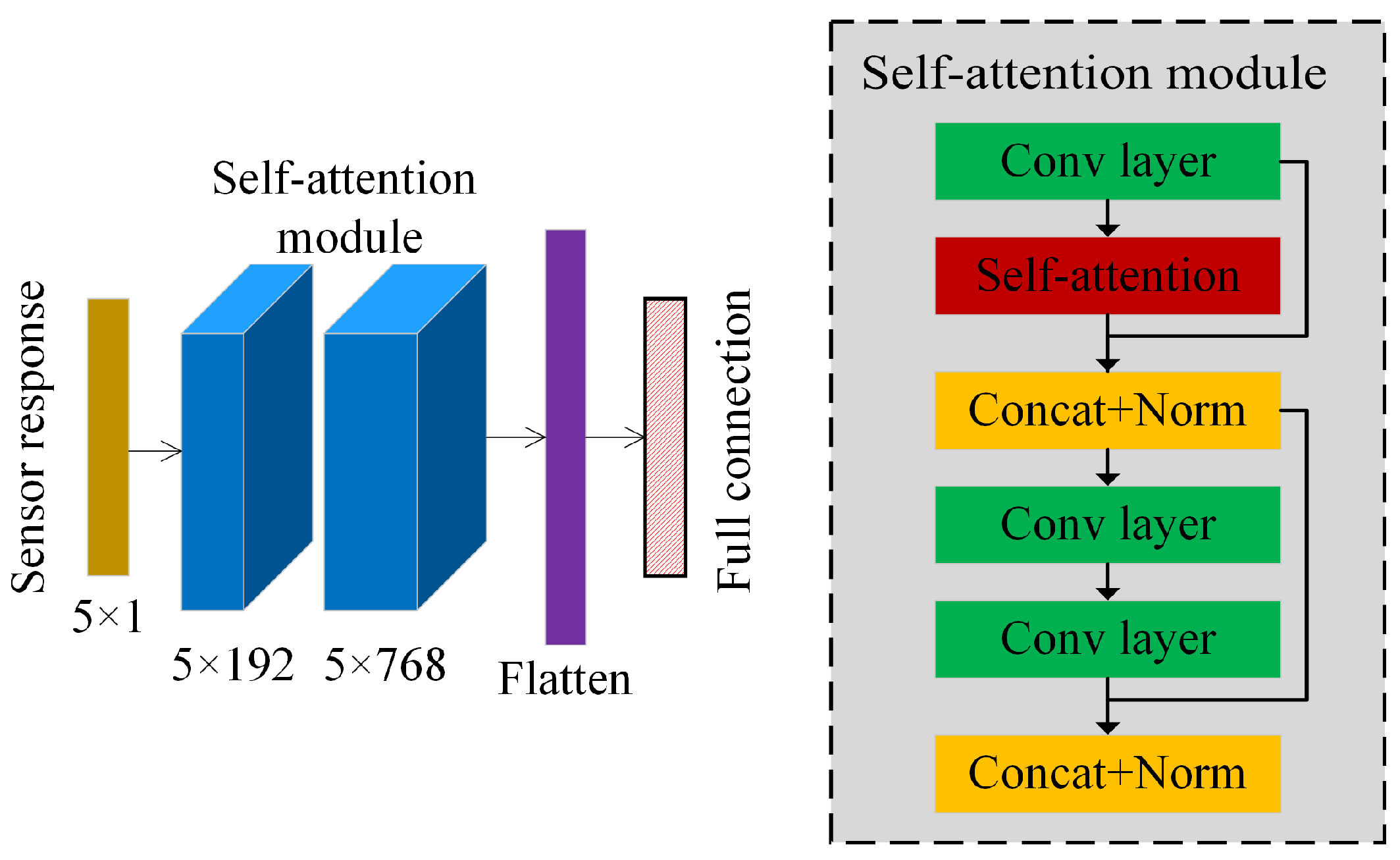
• We design an attention-based model for gas concentration estimation, utilizing the steady-state value of the sensor as input. This model achieves comparable accuracy to the CNN model while requiring fewer parameters.

The remainder of this paper is organized as follows. Section 2 describes the proposed method. Section 3 describes the experimental datasets and presents the results. Relevant discussions are presented in Section 4. Finally, Section 5 draws conclusions and highlights further research directions.

2. Proposed Method

Figure 1 illustrates the detailed structure of the proposed method. The proposed architecture comprises two main components: SSGAN and the target model T. The SSGAN consists of a generator G and a discriminator D. The generator is designed to produce both a synthetic sample and its corresponding label, while the discriminator determines whether the generated data are real or simulated. The generated data are subsequently fed into the target model for secondary training, aiming to mitigate the impact of imbalanced samples. The detailed structures of each model are described in the following sections.

2.1. Generator

The generator takes a set of normally distributed random noises $N^{b\ast d}$ as its input, where b and d represent the batch size and dimensions, respectively. The generator outputs a synthetic minority sample x and its corresponding label l, represented as $G\left(x\right)$ and $G\left(l\right)$, respectively. The model consists of three 1D convolution layers, a layer normalization layer, a leaky ReLU layer, an average pooling layer, and two output heads to obtain the output samples and labels simultaneously. The generator parameters are illustrated in Figure 2.

To optimize the generator, a specialized generative loss was designed, incorporating generative, within-class scatter, similarity, and distance losses.

The generative loss $L_{ger}$ is defined as follows:

$$L_{ger}=E_{x}logD\left(x\right)+E_{l}logD\left(l\right)$$

(1)

where $D\left(x\right)$ and $D\left(l\right)$ represent the recognition outputs of the discriminator, which aim to classify the generated samples and labels as true. $E_x$ and $E_l$ denote the identity matrix of the same dimensions as the input variables x and l.

The within-class scatter loss $L_w$ is designed to quantify the within-class scatter of the data and is formulated as follows:

$$L_w=\parallel Cov\left(x\right)-Cov\left(G\right(x\left)\right)\parallel +\parallel Cov\left(l\right)-Cov\left(G\right(l\left)\right)\parallel$$

(2)

where $Cov$ denotes the covariance matrix. The purpose of the within-class scatter loss is to constrain the inner-class distance of the generated data to be closer to a real instance.

The similarity loss $L_s$ enforces the generated data to exhibit a distribution similar to that of real instances, as defined by the following equation:

$$L_s=\parallel l_s(x,G\left(x\right))+\parallel l_s(l,G\left(l\right))$$

(3)

where $l_s(·)$ represents the cosine similarity metric. Similarity loss ensures that the direction of the generated data remains consistent with that of the real instance. Together, the similarity loss and within-class scatter loss impose a joint constraint on data generation, facilitating the approximation of the generated data distribution to real instances.

The distance loss $L_d$ is designed to restrict the generated data belonging to the minority data and is defined by the following equation:

$$L_d={\displaystyle \frac{1}{n}}\sum _{i=1}^n{\displaystyle \frac{\sqrt{{(x_i-G\left(x_i\right))}^2}}{x_i^{max}-x_i^{min}}}+{\displaystyle \frac{1}{n}}\sum _{i=1}^n{\displaystyle \frac{\sqrt{{(l_i-G\left(l_i\right))}^2}}{l_i^{max}-l_i^{min}}}$$

(4)

where n is the number of sensors. Typically, the generated data are distributed over the entire range of the sensor. The distance loss controls the generated data only in the range in which the minority lies. The ranges of the different sensors differ, which may cause the generated data to be more sensitive to a certain sensor. Therefore, we normalized each band of the generated data.

The full specific generative loss for generating the minority samples and their labels is given by the following equation:

$$L_G=L_{ger}+\alpha L_w+\beta L_s+\gamma L_d$$

(5)

where $\alpha$, $\beta$, and $\gamma$ are the weight coefficients for the within-class scatter, similarity, and distance loss terms, respectively. Invalid generated samples can emerge under two conditions: (1) the generated samples are overly concentrated in a single region, leading to uneven data distribution, or (2) the generated samples fall outside the real sensor range. Due to the constraints imposed by the specific generative loss function, the generator autonomously determines the optimal parameters. A detailed experimental analysis is provided in Section 4.2.

2.2. Discriminator

The discriminator functions as a binary classifier, distinguishing between real and generated input data. Two discriminators, $D_x$ and $D_l$, process samples and their corresponding labels separately. Although they have the same structure, they operate independently without parameter sharing. The model consists of two 1D convolutional layers, followed by a layer normalization module, a leaky ReLU layer, and a 30% dropout layer. The detailed parameters of the discriminator are illustrated in Figure 3, where n is the number of sensors and gases. The discriminator losses for $D_x$ and $D_l$ are defined in Equations (6) and (7).

$$L^{D_x}=E_{x}log{D}_x\left(x\right)+E_{x}log(1-D_x\left(G\left(x\right)\right))$$

(6)

$$L^{D_l}=E_{l}log{D}_l\left(l\right)+E_{l}log(1-D_l\left(G\left(l\right)\right))$$

(7)

The full discriminator loss function is formulated as follows:

$$L^D=L^{D_x}+L^{D_l}$$

(8)

2.3. Target Model

In this study, three types of neural networks were selected as the target models: BPNN, which was the first gas concentration estimation model for experimental data in this study [35]; CNN, which is the most widely used model [6]; and a recently developed attention-based model. The attention model enhances accuracy by analyzing the characteristics of different gases [36]. However, existing attention-based models primarily focus on dynamic response signals, which capture rich features but overlook commonly used steady-state values. To address this limitation, an attention model based on steady-state values was designed for gas concentration estimation in this study. The parameters of the BPNN and CNN are illustrated in Figure 4.

The proposed attention model consists of two self-attention modules and an output head. Each self-attention module assigns weights to each channel before extracting final feature representations using two convolutional layers. The self-attention and convolutional layers are integrated into the ResNet [37] to mitigate model degradation. The detailed structure of the model is shown in Figure 5.

The convolutional layer parameters for the two self-attention modules were set to 64–32–64 and 256–128–256, respectively, with an attention head size of 8. In this model, layer normalization was applied to standardize the sample features. All target models follow an end-to-end architecture, utilizing the raw response signals from the sensor array as input without any preprocessing.

2.4. Model Training with Outcome Assessment Strategy

An outcome assessment strategy was designed to evaluate the performance of the proposed SSGAN.

Initially, the target model was trained on raw imbalanced experimental data to obtain baseline convergence results. Establishing a specific class criterion for measuring data balance is challenging due to the discrete nature of labels and the varying concentration ranges of different gases. To address this, we defined minority class samples as those whose mean absolute percentage error (MAPE) in the overall test dataset exceeded a predefined threshold $\Theta$. This approach eliminates the need for explicit gas concentration classification. The number of synthetic samples required for generation by SSGAN was determined by comparing the number of minority class samples with the remaining samples. Generator G and discriminator D were updated through adversarial training based on both generated and minority class samples, as defined in the following equation:

$$\underset{G}{argmax{L}_G}=\underset{G}{argmax{L}_{ger}+\alpha L_w+\beta L_s+\gamma L_d}$$

(9)

The target model from the first iteration is retrained using the generated data and real instances to obtain the final optimized results.

3. Experiments

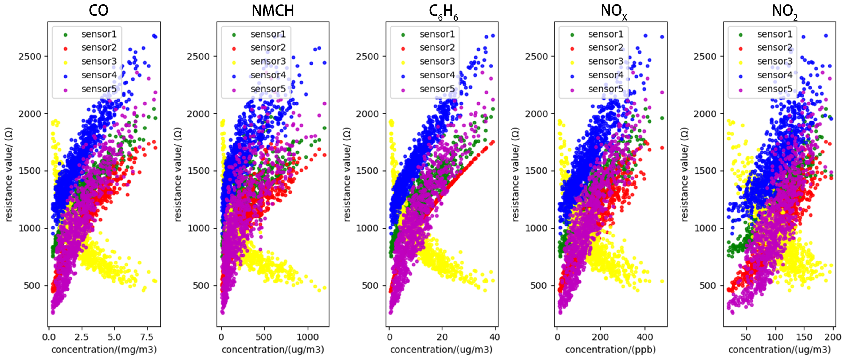
3.1. Dataset Description

The Air Quality dataset was obtained from the UC Irvine Machine Learning Repository [38]. It consists of responses from seven sensors deployed outside an Italian city and high-precision concentrations of five gases. The dataset contains 9357 instances of hourly averaged responses from an array of five metal oxide chemical, temperature, and humidity sensors. The sensor array detected carbon monoxide (CO), non-methanic hydrocarbons, benzene, total nitrogen oxide ($N{O}_x$), and nitrogen dioxide ($N{O}_2$) concentrations, and the truth gas concentration was provided by a colocated reference certified analyzer. In this study, the effects of temperature and humidity were not considered.

Due to the presence of missing values in the dataset, only complete sensor and gas concentration data were used for experimentation. From the complete instances, a subset was randomly selected to construct the training dataset, while the remaining instances were allocated for testing.

As references for the experimental analysis, Figure 6 illustrates the sensitivity of each sensor to the different gases. The results indicate that the five chemical sensors exhibit a strong correlation with their respective target. Additionally, prior research has demonstrated the temporal drift of these sensors [39].

3.2. Experimental Setting

The dataset included 827 complete examples; the remaining were missing data. Among the complete examples, 579 were randomly selected for training, and the remaining were used for testing. For the target model, the loss function was set to mean-square error (MSE), and the optimizer was Adam. The learning rate was set to 1 × ${10}^{-4}$ for both the target model and generator and 1 × ${10}^{-5}$ in the discriminator, and the batch size was 32. The iteration number of the CNN and attention model was set to 200, and that of the BPNN was set to 10,000. For the SSGAN, 32 examples were selected as one patch, and the Adam optimizer was used. The iteration number was 2000, with a generator learning rate of 1 × ${10}^{-4}$ and a discriminator learning rate of 1 × ${10}^{-5}$. A lower discriminator learning rate can improve the stability of SSGAN during training. The hyperparameters $\alpha$, $\beta$, and $\gamma$ in Equation (5) are 0.003, 0.3, and 10, respectively. The threshold $\Theta$ was set to 0.5, and the random noise dimension was set to 128 × 1.

In the following experiments, the mean absolute error (MAE), MSE, and mean relative error (MRE) were used to evaluate the performance of the target model on both real and generated examples. MAE measures the average absolute deviation of the predicted values and is less sensitive to outliers. MSE, by squaring the errors, is more sensitive to outliers than MAE. MRE is primarily used to assess the relative error, minimizing the influence of varying gas concentration ranges on evaluation metrics. The performance of the target model was analyzed based on improvements in accuracy when trained with the generated examples.

3.3. Experimental Results

3.3.1. BPNN Results

Figure 7 shows the initial training results of the BPNN target model. The BPNN effectively estimated the concentrations of most gases, achieving MAE, MRE, and MSE of 67.2075, 117.9375, and 18,624.09, respectively. However, compared to the other two target models, the BPNN demonstrated the lowest prediction accuracy. Additionally, the BPNN model required the normalization of each sensor response for convergence; otherwise, the model failed to achieve optimal results. Notably, the model performed best when predicting a single gas concentration, necessitating five separate training runs. For larger gas sensor drifts (NMHC and ${\mathrm{NO}}_X$), the training iterations of the BPNN were also significantly higher than those of the rest of the target models. Following testing, NMHC converged after 3000 iterations, while ${\mathrm{NO}}_X$ converged after 1800 iterations.

Figure 8 presents the minority class samples generated by the generator for the BPNN target models. Compared to real instances, the generated samples exhibit a uniform distribution within the corresponding input data space. A closer inspection reveals that the generated data follow the same directional trend as the real instances, suggesting a high degree of cosine similarity between them. Additionally, none of the generated samples exceeded the expected physical range, maintaining consistency with real-world constraints.

Figure 9 presents the results of the proposed SSGAN method applied to the BPNN target model. For evaluation, MAE, MSE, and MRE values were computed for both the target model and the SSGAN results. Compared to the initial training results, MAE, MRE, and MSE increased by 4.45%, 3.72%, and 8.76%, respectively. Based on the analysis of these metrics, it can be concluded that the SSGAN model effectively mitigates the influence of imbalanced samples on the BPNN model, thereby improving its predictive accuracy. However, an anomaly was observed in NMHC gas: Sensor-1-generated samples were most concentrated on one side, and the drift samples were empty on the other side. This was the main reason for the reduced accuracy of NMHC in the SSGAN results.

Table 1. Evaluation metrics for BPNN.

Model	Metrics	CO	NMHC	C6H6	${\mathbf{NO}}_{\mathit{x}}$	${\mathbf{NO}}_2$	Mean
BPNN	MAE	1.5081	203.1564	8.1824	88.3552	34.8352	67.2075
	MRE	99.2208	192.5111	157.1520	97.8494	42.9541	117.9375
	MSE	3.7009	78,250.9600	109.6785	12,875.4700	1880.6373	18,624.09
BPNN + SSGAN	MAE	1.4495	203.6666	7.6831	81.7475	32.9960	65.5085
	MRE	96.5658	196.6645	148.7511	89.4066	41.1859	114.5148
	MSE	3.4834	77,245.9300	96.0657	10,965.9370	1701.6248	18,002.6074
Enhancement (%)	MAE	3.89	−0.25	6.10	7.48	5.28	4.45
	MRE	2.68	−2.15	5.34	8.63	4.12	3.72
	MSE	5.88	1.28	12.41	14.83	9.2	8.76

summarizes the gas concentration estimation accuracies of the BPNN model and SSGAN.

3.3.2. CNN Results

Figure 10 presents the initial training results of the CNN target model. The MAE and MSE of the CNN model were optimal at 12.4896 and 659.3767, respectively. From a qualitative perspective, its prediction results were the closest to the ground truth, with relatively few outliers. However, when compared with the other four gases, the prediction error for CO was slightly lower than that of the attention model. Specifically, the MAE and MSE for CO decreased by 0.21 and 0.38, respectively.

Figure 11 shows the generated samples produced by the generator for the CNN target model. The generated samples exhibited a high degree of correlation with real instances. However, slight differences were observed in the dispersion of the generated data compared to the real instances, particularly for ${\mathrm{NO}}_2$, which demonstrated significant dispersion (see Figure 11). The generated data tended to cluster closer to the central plane, leading to a reduced interclass distance. This, in turn, resulted in fewer “effective” generated data points, potentially limiting the optimization capacity of the SSGAN model for ${\mathrm{NO}}_2$ gas. It is hypothesized that this limitation may be influenced by batch size. The batch size determines the amount of data used by $L_w$ to compute within-class separability, meaning that larger batch sizes allow $L_w$ to better approximate the overall distribution of real instances. This observation aligns with prior conjectures regarding the impact of generated data on SSGAN performance.

Figure 12 presents the results of the proposed SSGAN method applied to the CNN target model. Compared to the initial training results, MAE, MRE, and MSE increased by 12.06%, 35.92%, and 19.51%, respectively. The results indicate that the SSGAN-enhanced predictions were closer to the actual gas concentrations, particularly for CO, C₆H₆, and ${\mathrm{NO}}_X$ gases. In addition, the outliers significantly improved, and the MSE of the first four gases decreased by 73.86%, 18.92%, 54.13%, 23.89%, and 4.68%. However, the improvement in ${\mathrm{NO}}_2$ gas was much lower than those of the remaining four gases. The specific gas prediction accuracies are presented in

Table 2. Evaluation metrics for CNN.

Model	Metrics	CO	NMHC	C6H6	${\mathbf{NO}}_{\mathit{x}}$	${\mathbf{NO}}_2$	Mean
CNN	MAE	0.4417	32.0820	0.7760	20.0776	9.0806	12.4896
	MRE	17.2745	24.9271	19.0617	18.3452	10.4591	18.0207
	MSE	0.5121	2384.297	1.0802	772.6922	138.3014	659.3767
CNN + SSGAN	MAE	0.2526	27.9720	0.4084	17.7480	8.5353	10.9832
	MRE	12.7600	15.5680	5.7231	14.3212	9.3658	11.5476
	MSE	0.1337	1933.2006	0.4955	588.1096	131.8301	530.754
Enhancement (%)	MAE	42.82	12.81	69.98	11.60	6.00	12.06
	MRE	26.14	37.55	46.68	21.93	10.76	35.92
	MSE	73.86	18.92	54.13	23.89	4.68	19.51

.

3.3.3. Attention Model Results

Figure 13 presents the initial training results of the attention model. The MRE of the attention model was the lowest among the three target models, at 14.73, indicating that its approximation curve for gas concentrations was the closest to the ground truth. In contrast, higher MAE and MSE values suggest the presence of more outliers. The core concept of the attention model proposed in this study is to analyze the interference of sensor cross-sensitivity on gas concentration estimation. However, for the dataset used in this study, each sensor responded to five gases. Thus, even though the MRE of the attention model achieved its optimal value, the model’s effectiveness requires further exploration.

Table 3. Evaluation metrics for attention models.

Model	Metrics	CO	NMHC	C6H6	${\mathbf{NO}}_{\mathit{x}}$	${\mathbf{NO}}_2$	Mean
Attention model	MAE	0.2234	37.0816	0.8511	22.3352	9.9708	14.0924
	MRE	11.3531	19.0948	12.2931	19.3524	11.5774	14.7342
	MSE	0.1298	3695.0596	1.4793	994.2543	171.1836	972.4214
Attention model + SSGAN	MAE	0.2307	36.2352	0.8492	20.9190	9.8505	13.6169
	MRE	11.6757	18.6365	15.1697	16.2638	11.1091	14.5708
	MSE	0.1279	3529.2622	1.3503	922.4245	174.0809	925.4491
Enhancement (%)	MAE	−3.35	2.28	0.22	6.34	1.21	3.38
	MRE	−2.84	2.40	−23.4	15.96	4.04	1.11
	MSE	1.47	4.49	8.71	7.22	−1.69	1.84

provides the gas concentration estimation accuracies of the attention model.

The results of the generator are shown in Figure 14. The generated samples are generally similar to the examples; however, there are still some problems with NMHC and ${\mathrm{NO}}_2$. The estimation accuracy of NMHC and ${\mathrm{NO}}_2$ gases continuously decreased owing to time drift. However, it is difficult for the generative model to learn the changes in the time series; therefore, the generated samples have certain distribution differences. In addition, there were relatively fewer gas samples with high concentrations than those with lower concentrations in the generated samples. Balancing the proportion of samples generated at different concentrations is a direction for future improvement.

Figure 15 shows the proposed SSGAN method results of the attention model. Compared to the initial training results of the attention model, the MAE, MSE, and MRE were improved by 3.38%, 1.11%, and 1.84% in the SSGAN model, respectively. The primary error in the initial attention model stemmed from the high-concentration gases. After secondary training, the accuracy of the attention model in estimating high-concentration gases improved, as shown in Figure 15. Although high-concentration gas samples represent a small fraction of the total sample set, the model’s accuracy improvement is relatively modest. However, the enhancement in the estimation accuracy of high-concentration samples underscores the effectiveness of the SSGAN model. Table 3 presents the gas concentration estimation accuracies for both the attention model and SSGAN. Additionally, a manually collected dataset is provided to verify the robustness of the model. The sensor response values were obtained from two commercial sensors, and the target gases were a mixture of ethanol and formaldehyde. The dataset consists of 100 samples, and Figure

Table A1. Evaluation metrics for attention models of manually collected dataset.

Model	Metrics	Formaldehyde	Ethanol	Mean
Attention model	MAE	0.0048	0.0203	0.0126
	MRE	0.7300	1.5978	1.1639
	MSE	0.00004	0.0006	0.0003
Attention model + SSGAN	MAE	0.0046	0.0124	0.0085
	MRE	0.7153	1.02952	0.8724
	MSE	0.00003	0.0002	0.0001
Enhancement (%)	MAE	4.62	39.08	32.47
	MRE	2.01	35.57	25.05
	MSE	31.92	64.65	62.50

and Figure A5 in Appendix B detail the specific results of the experiment.

The above analysis demonstrates that SSGAN can effectively generate training data. However, when the gas composition is overly complex, sensor responses may be similar even though the gas concentrations differ due to inherent cross-sensitivity. SSGAN cannot handle situations where one input corresponds to multiple outputs, which can lead to reduced accuracy or even failure to converge. This limitation may be a potential weakness of the SSGAN models.

4. Discussion

4.1. Imbalanced Samples Analysis

In this section, we investigate whether imbalanced samples are the primary cause of model degradation:

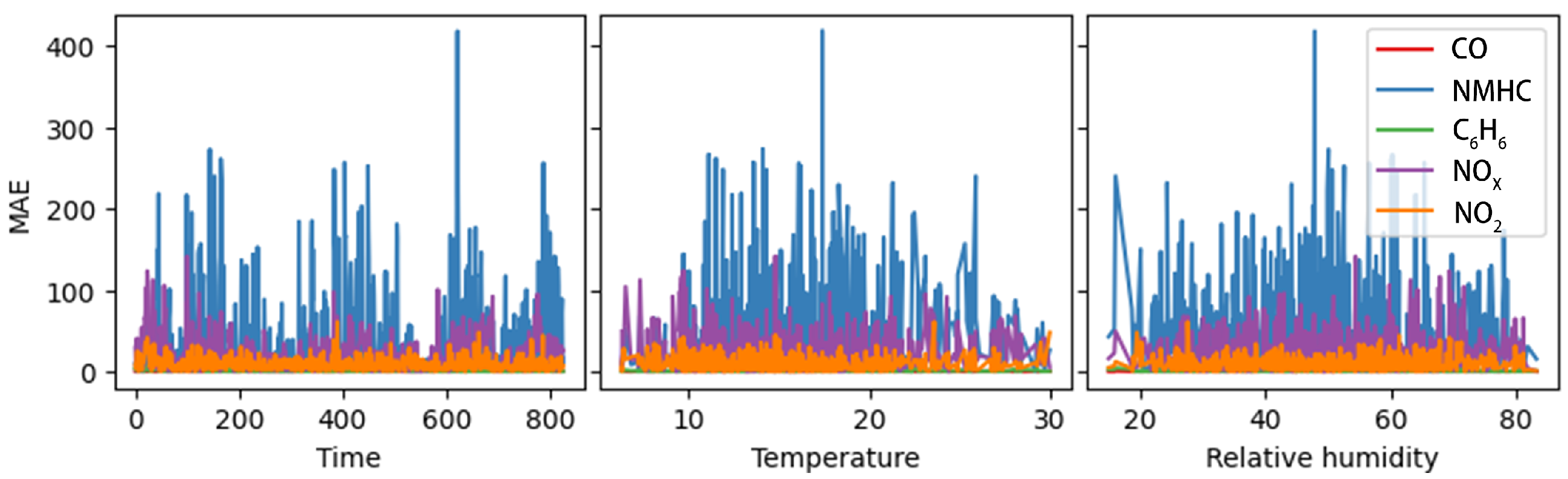
• Sensor drift: Sensors experience drift in sensitivity due to environmental factors such as time, temperature, and humidity, resulting in inconsistent sensor responses. This could contribute to degraded model performance. Figure 16 illustrates the relationship between gas identification accuracy and time, temperature, and humidity in the target model. We observe that model accuracy does not significantly change under varying sensor drifts caused by time, temperature, and humidity. Therefore, when sensor drift data are included in the training set, the target model shows a degree of localized robustness against these interferences. As a result, the error in gas concentration identification exhibits a low correlation with sensor drift;
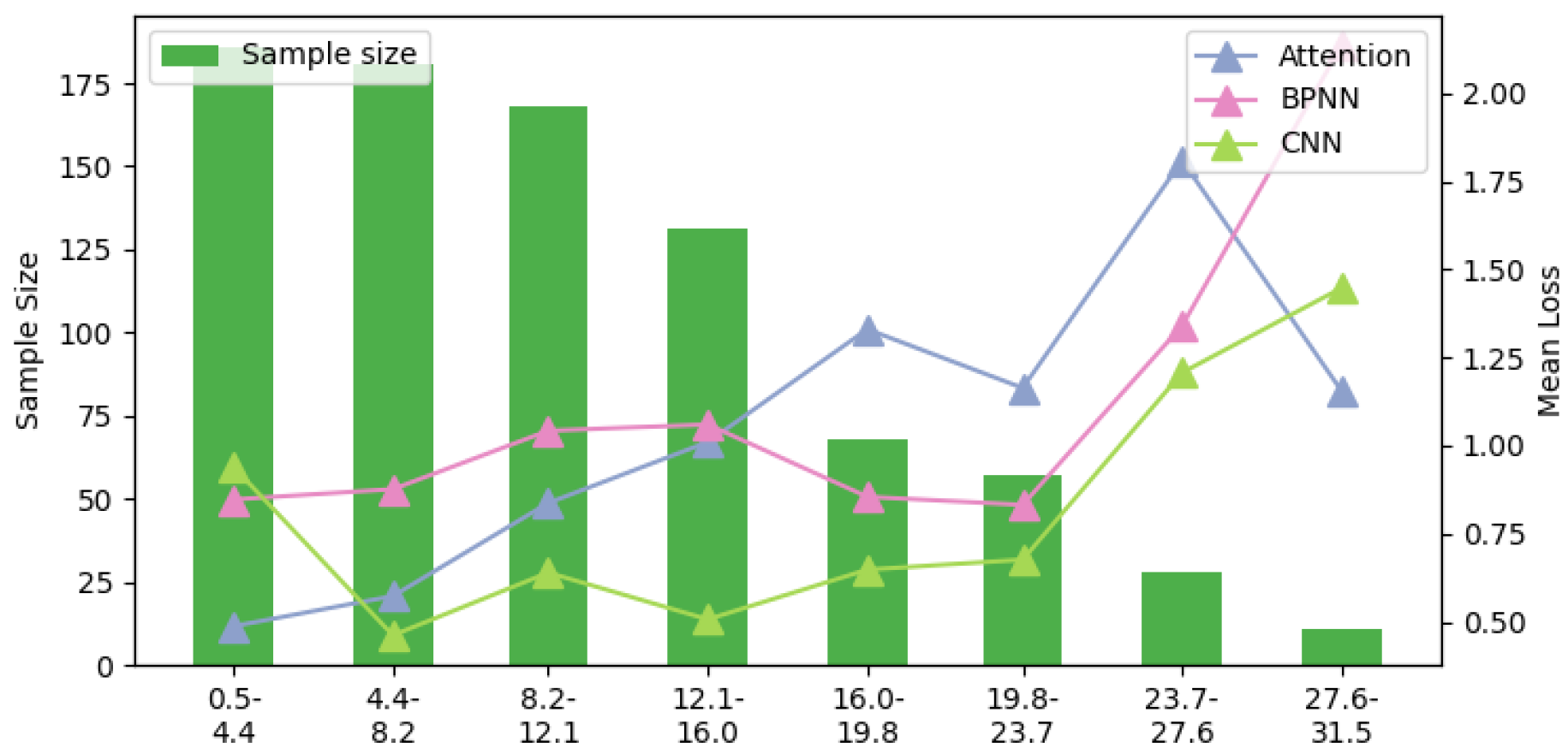
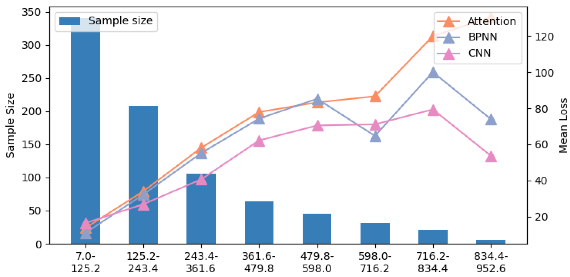
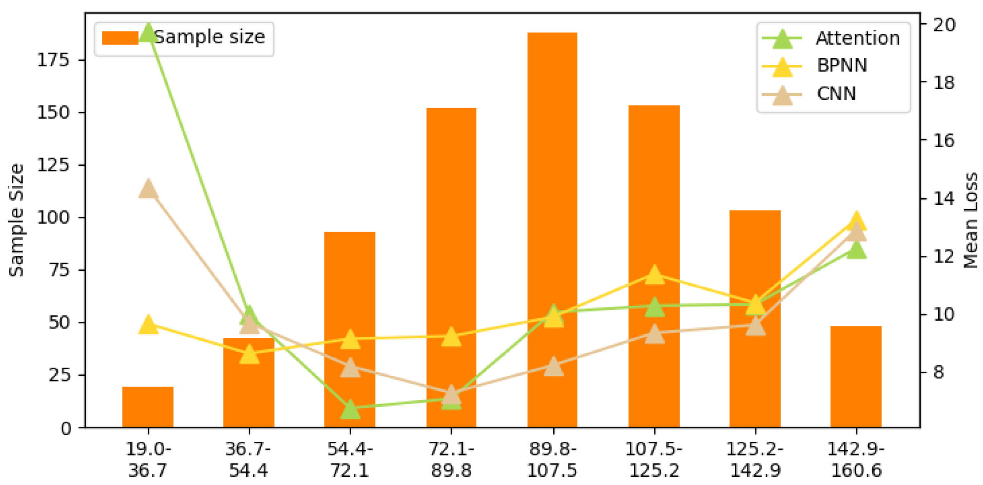
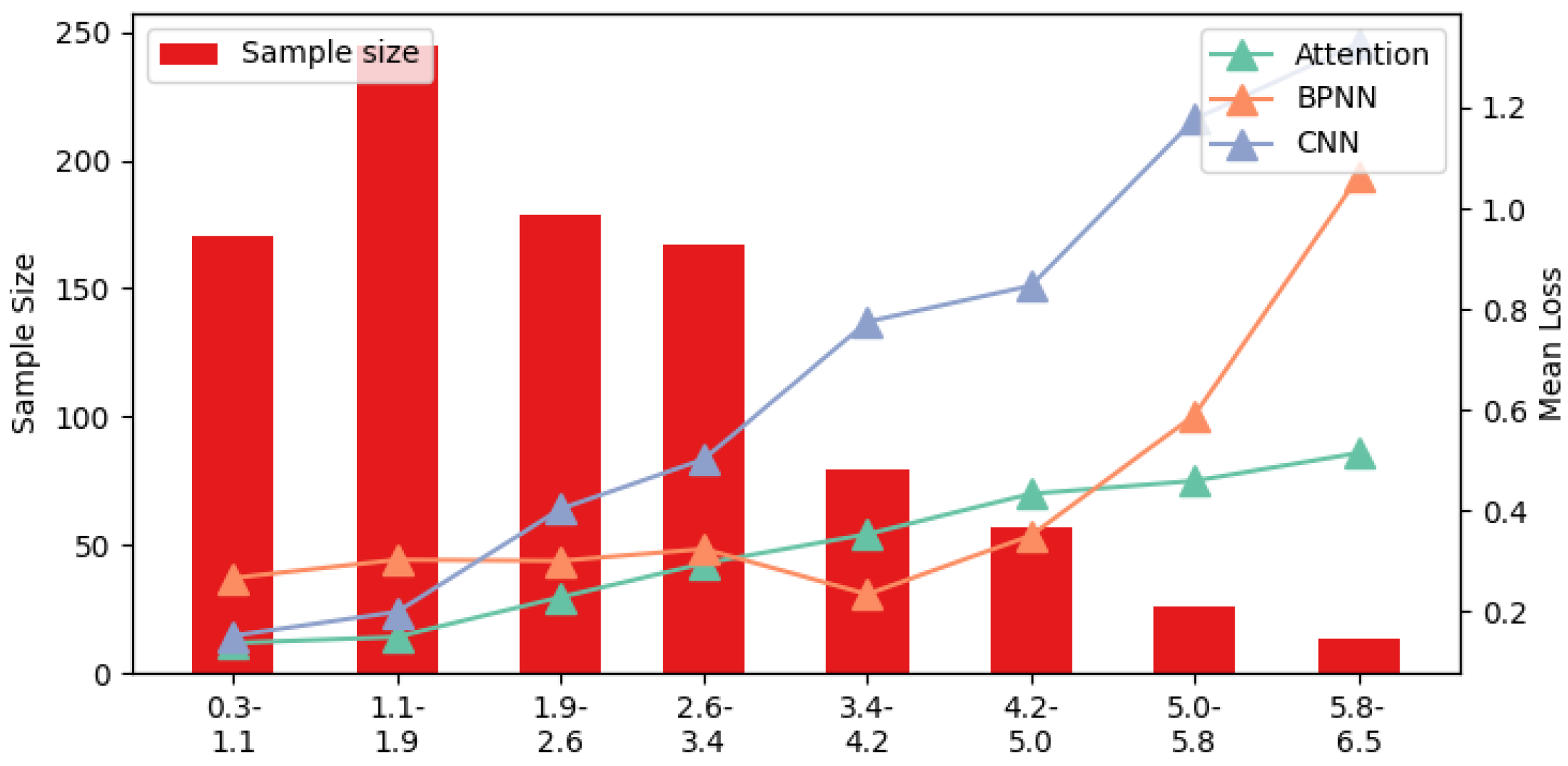
• Imbalanced samples: In long-term gas detection, the gas concentration tends to remain stable, with minimal fluctuations. This results in imbalanced gas concentration data, which can lead to bias in the gas concentration estimation model. Figure 17 shows the accuracy of the target model under different CO gas concentrations (relationships for other gases are provided in Appendix A, Figure A1, Figure A2, Figure A3 and Figure A4). In Figure 17, a significant negative correlation between gas concentration and accuracy is observed, confirming that sample imbalance negatively impacts the accuracy of the target model.

4.2. Study of Specific Generative Loss

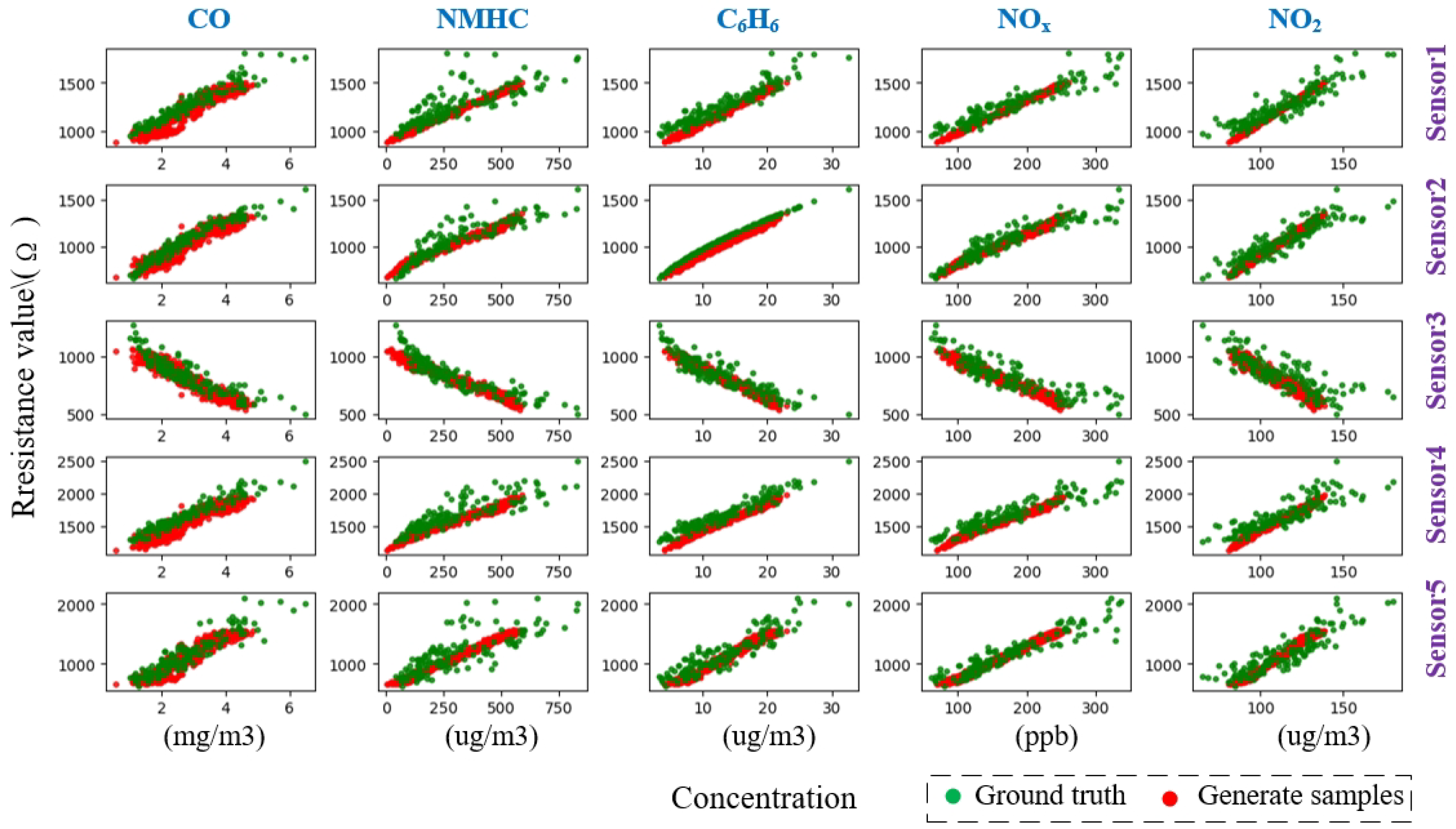
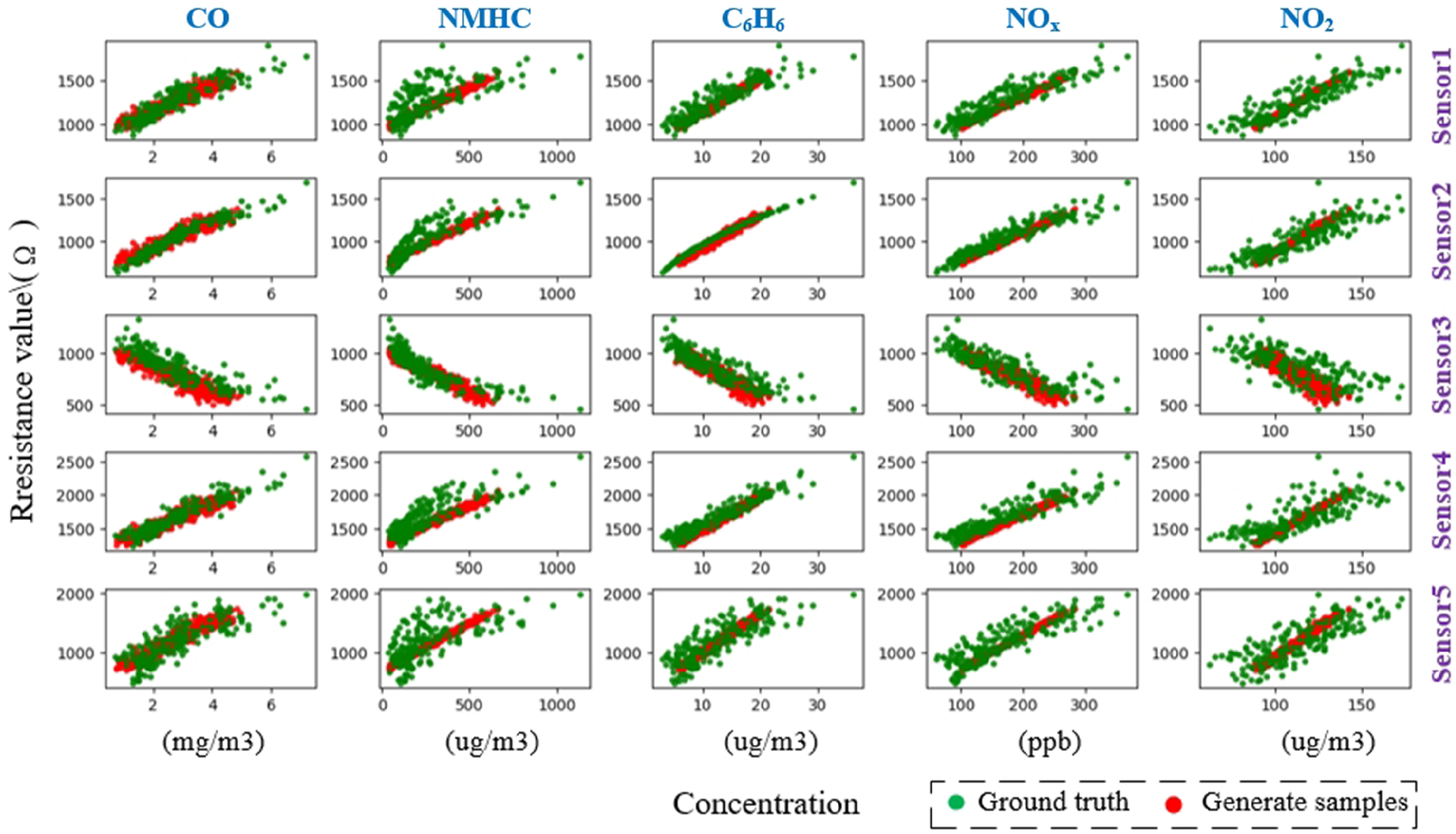
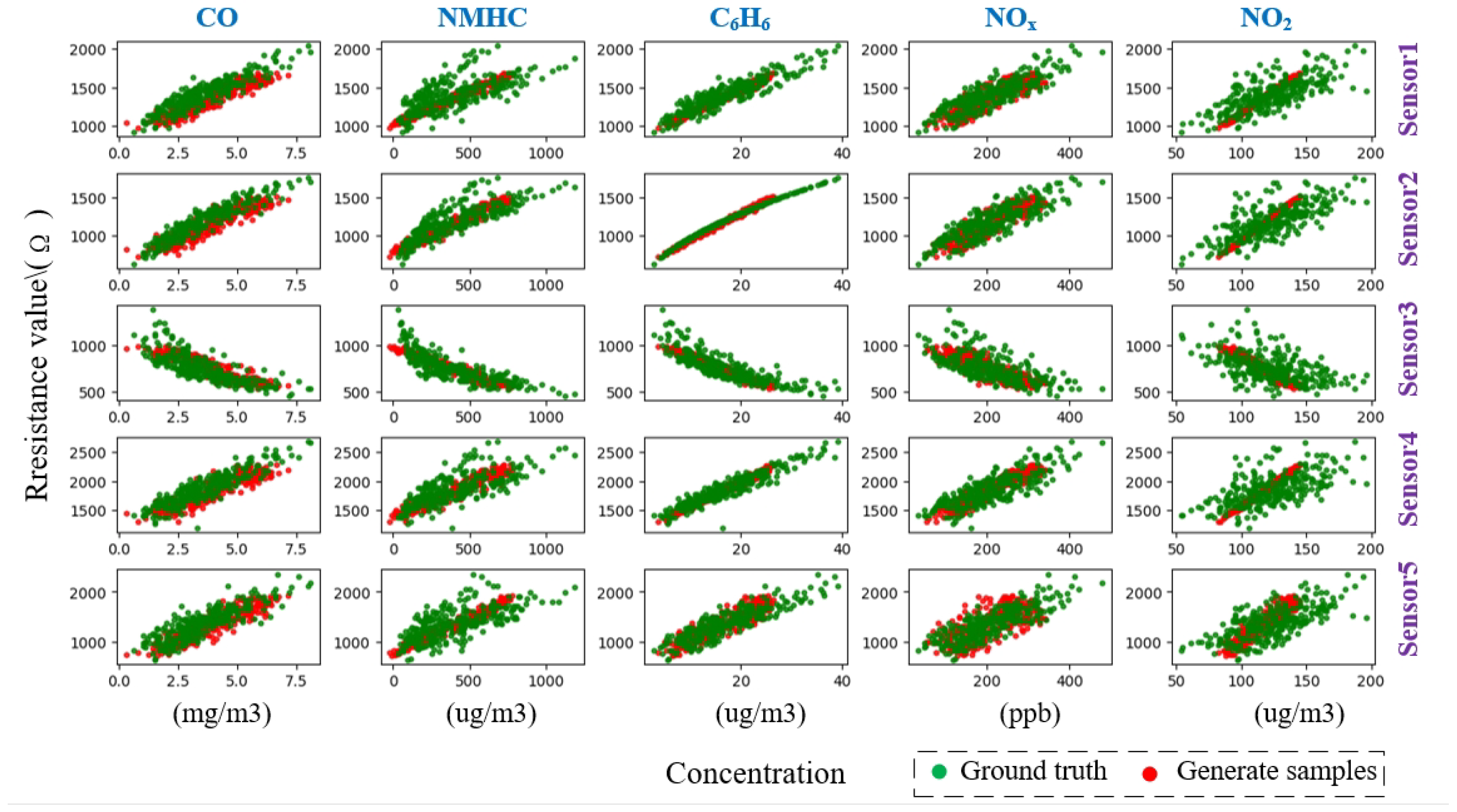
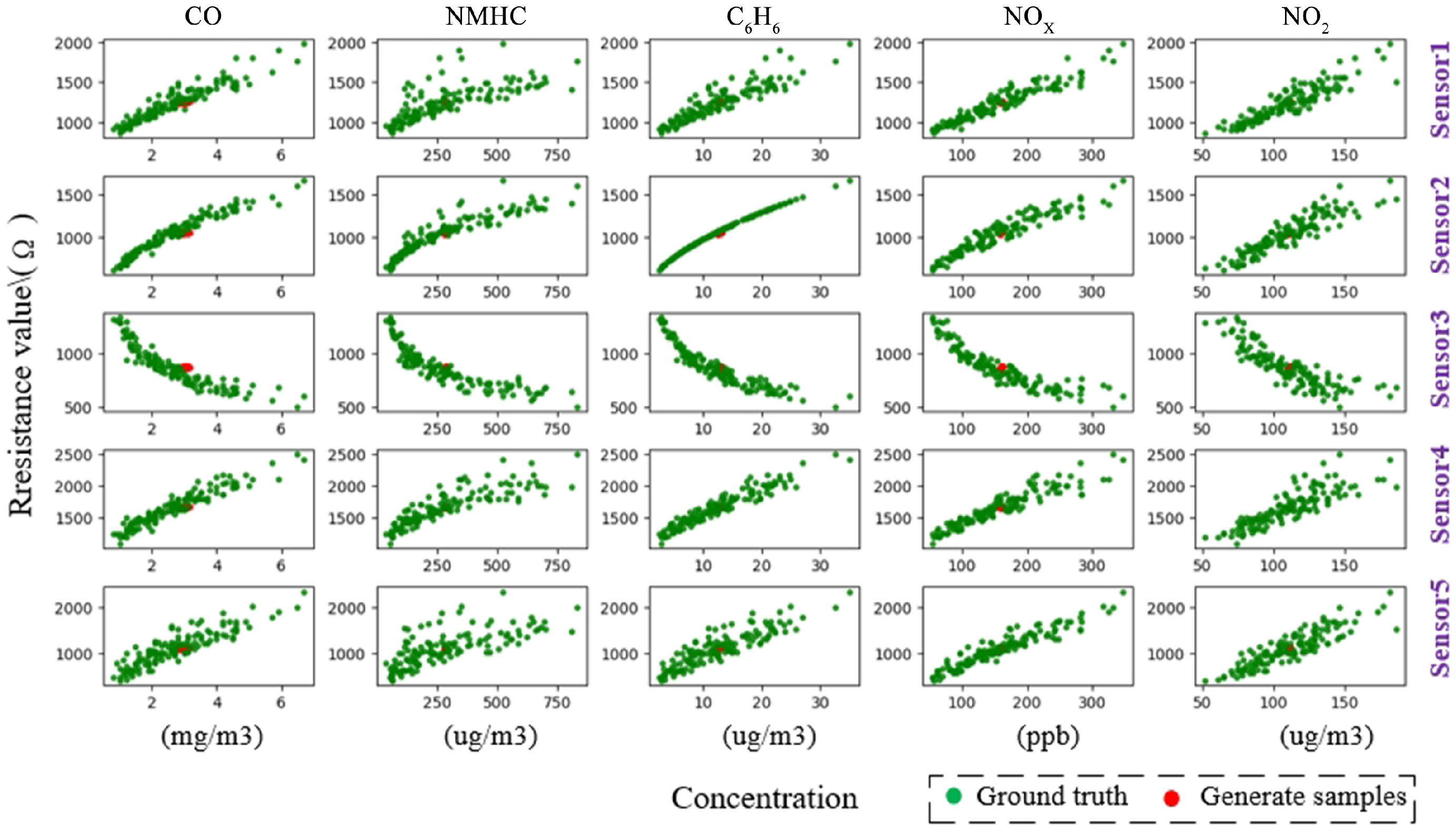
Specific generative loss can help to make generated samples more similar to real instances. To further illustrate the influence of the specific generative loss term on sample generation, we discuss the three losses defined in Equations (2)–(4):

• Within-class scatter loss $L_w$: Figure 18 shows the study of within-class scatter loss. The colors represent the samples generated by the SSGAN model. In Figure 18, the color on all subfigures has a similar trend. The generator without $L_w$ can only generate the central sample in the training set. Although the generated sample is similar to the instant, the variance in sensor response and gas concentration is different. This results in an absence of abnormally high-concentration gas samples, which was expected in this study. During the training of the target model, this could lead to overfitting and performance degradation. Therefore, the generative loss function requires an additional constraint on inter-class separability;
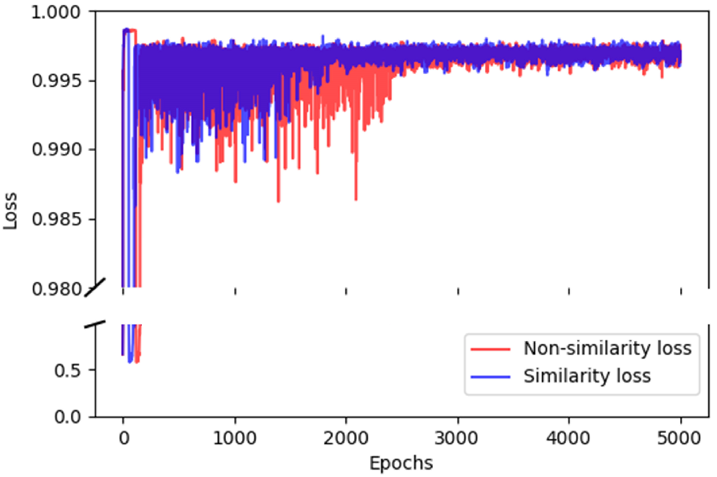
• Similarity loss $L_s$: Figure 19 contrasts the effect of the similarity loss on the cosine similarity of the generated samples. We can see that the cosine similarity results of the specific generative loss and none $L_s$ are generally the same, but their decline rates are different. The specific generative loss achieved the lowest cosine similarity after 1700 epochs, which is reduced by 500 epochs compared to no $L_s$. This observation illustrates the similarity loss function can better guide the model training. Additionally, we observe that the cosine similarity of $L_s$ is slightly higher than the loss function without $L_s$, possibly because the $L_s$ makes the model focus more on the direction of vector similarity;
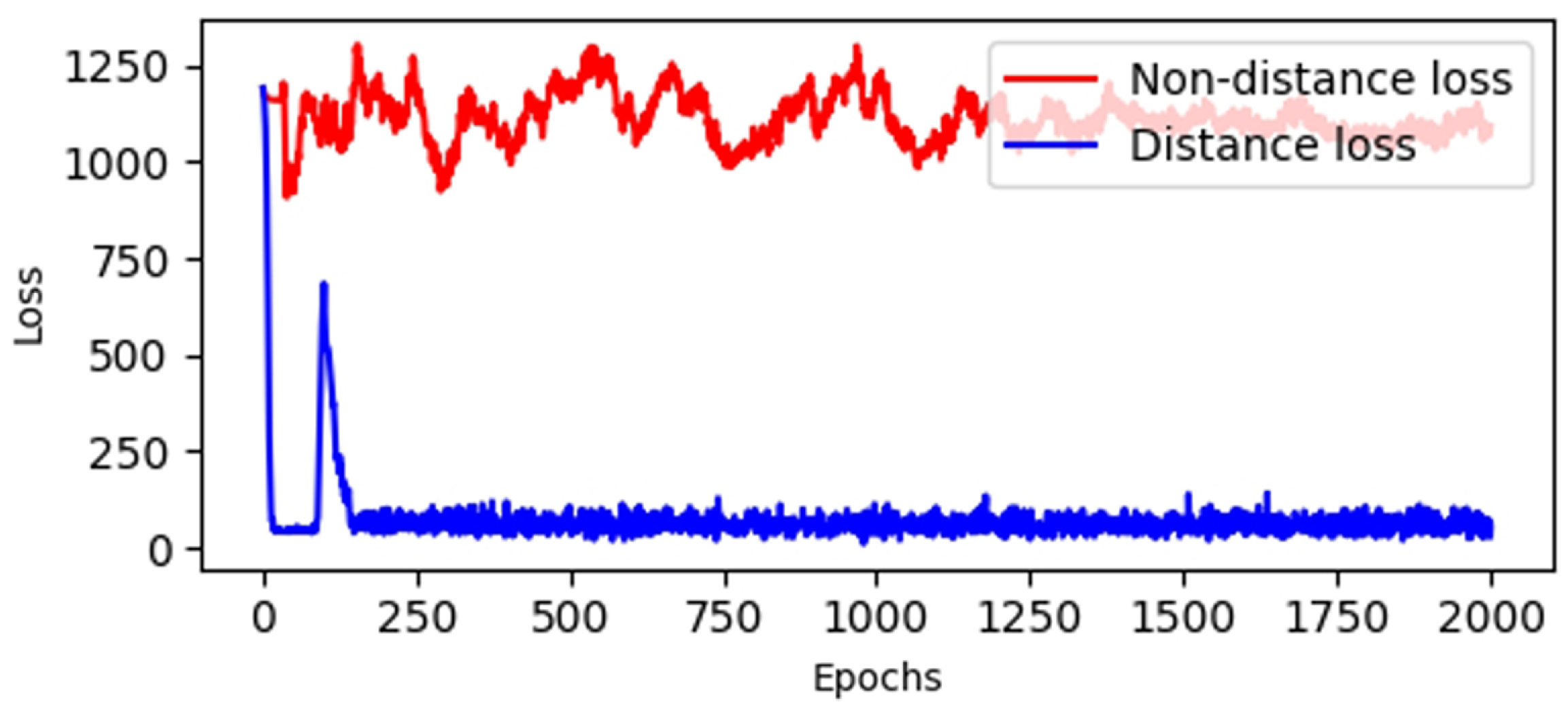
• Distance loss $L_d$: Distance loss constrains the generated data to stay within the range of real sensor responses and gas concentrations. To illustrate the influence of the distance loss term on generated samples, we analyzed the distance between the generated samples and real instances, both with and without the distance loss term. Figure 20 shows the change curve of distance loss for each epoch. We observe that the generated samples without $L_d$ have an average Euclidean distance of 1200 from the real instances, placing the results outside the expected range of the sensor response. In contrast, when the specific generative loss includes $L_d$, the distance is significantly reduced to 150, ensuring that the generated samples adhere more closely to the real data distribution. Therefore, the distance loss improves the generator’s ability to constrain the desired range of generated data;
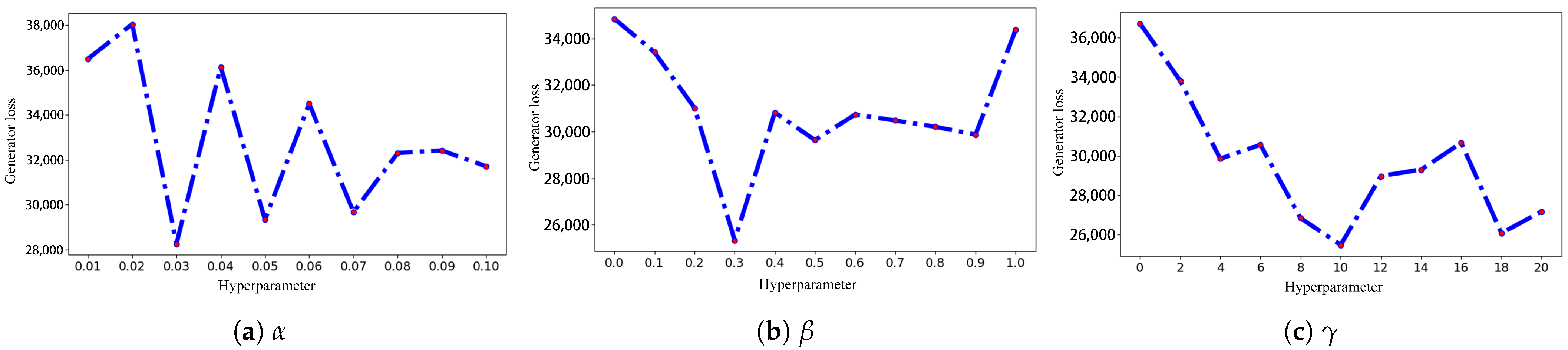
• Hyperparameter study: Figure 21 presents the study of the three hyperparameters in Equation (5): $\alpha$, $\beta$, and $\gamma$. In Figure 21, $\alpha$, $\beta$, and $\gamma$ range from 0.01 to 0.1, 0 to 1, and 0 to 20, respectively. When the value of hyperparameters is 0, the specific generative loss is not utilized, as discussed in the previous section. We can clearly see that the curve between hyperparameters and generator loss on the three subfigures has a similar trend. The generator loss decreases gradually as the hyperparameter increases. Upon reaching an optimal value, the generator loss begins to increase and ultimately stabilizes. Therefore, values of 0.03, 0.3, and 10 for $\alpha$, $\beta$, and $\gamma$ yield better-generated samples.

4.3. Study of Existing Data Augmentation Methods

In this section, we compare the proposed method with several existing data augmentation techniques to demonstrate its effectiveness.

Table 4. Data augmentation method.

Method	Input Data	Output Data
CTGAN [29]	Random noise	Features
SMOTE [24]	Minority samples	New samples
VAEs [40]	Minority samples	New samples
Over sampling [41]	Dataset	Enhanced dataset
Under sampling [25]	Dataset	Reduced dataset

summarizes the input and output of data augmentation methods used in recent years. While research on imbalanced samples has gained traction, studies specifically addressing gas sensors remain limited [29]. Moreover, most generative models only generate samples, and the corresponding labels are manually annotated. Methods such as SMOTE, which generate new samples based on the neighborhood of minority class samples, are not directly applicable to gas sensors due to their cross-sensitivity, which prevents accurate gas concentration estimation. Similarly, the limited volume of gas sensor data prevents effective resampling. Therefore, the SSGAN model shows significant potential for further research in this area.

5. Conclusions and Future Work

In this study, we propose an SSGAN model to mitigate the degradation of gas concentration estimation models caused by imbalanced samples. A specific generative loss function was designed to train the proposed SSGAN. This loss function allows the network to generate synthetic samples along with their corresponding labels, ensuring that the generated samples share the same distribution and range as the real instances. Additionally, an attention model was designed to estimate multiple gas concentrations directly using raw sensor responses as inputs. The proposed SSGAN was tested on an Air Quality dataset, and the results demonstrate that the method effectively reduces the impact of imbalanced samples on model accuracy.

Although the proposed method has been shown to be feasible and effective, the experimental results indicate that the generator struggles to control the proportion of samples at different gas concentrations. Therefore, managing the distribution of generated samples at various gas concentrations remains a key area for future research.

References

1. Tan, J.; Xu, J. Applications of electronic nose (e-nose) and electronic tongue (e-tongue) in food quality-related properties determination: A review. Artif. Intell. Agric. 2020, 4, 104–115. [Google Scholar]
2. Di Natale, C.; Macagnano, A.; Davide, F.; D’amico, A.; Paolesse, R.; Boschi, T.; Faccio, M.; Ferri, G. An electronic nose for food analysis. Sens. Actuators B Chem. 1997, 44, 521–526. [Google Scholar]
3. Dragonieri, S.; Annema, J.T.; Schot, R.; van der Schee, M.P.; Spanevello, A.; Carratú, P.; Resta, O.; Rabe, K.F.; Sterk, P.J. An electronic nose in the discrimination of patients with non-small cell lung cancer and COPD. Lung Cancer 2009, 64, 166–170. [Google Scholar]
4. Montuschi, P.; Mores, N.; Trové, A.; Mondino, C.; Barnes, P.J. The electronic nose in respiratory medicine. Respiration 2012, 85, 72–84. [Google Scholar] [PubMed]
5. Baldwin, E.A.; Bai, J.; Plotto, A.; Dea, S. Electronic noses and tongues: Applications for the food and pharmaceutical industries. Sensors 2011, 11, 4744–4766. [Google Scholar] [CrossRef]
6. Robin, Y.; Amann, J.; Baur, T.; Goodarzi, P.; Schultealbert, C.; Schneider, T.; Schütze, A. High-performance VOC quantification for IAQ monitoring using advanced sensor systems and deep learning. Atmosphere 2021, 12, 1487. [Google Scholar] [CrossRef]
7. Liu, H.; Li, Q.; Yu, D.; Gu, Y. Air quality index and air pollutant concentration prediction based on machine learning algorithms. Appl. Sci. 2019, 9, 4069. [Google Scholar] [CrossRef]
8. Furizal, F.; Ma’arif, A.; Firdaus, A.A.; Rahmaniar, W. Future Potential of E-Nose Technology: A Review. Int. J. Robot. Control. Syst. 2023, 3, 449–469. [Google Scholar]
9. Chen, Z.; Zheng, Y.; Chen, K.; Li, H.; Jian, J. Concentration estimator of mixed VOC gases using sensor array with neural networks and decision tree learning. IEEE Sens. J. 2017, 17, 1884–1892. [Google Scholar]
10. Fan, S.; Li, Z.; Xia, K.; Hao, D. Quantitative and qualitative analysis of multicomponent gas using sensor array. Sensors 2019, 19, 3917. [Google Scholar] [CrossRef]
11. Zimmerman, N.; Presto, A.A.; Kumar, S.P.; Gu, J.; Hauryliuk, A.; Robinson, E.S.; Robinson, A.L.; Subramanian, R. A machine learning calibration model using random forests to improve sensor performance for lower-cost air quality monitoring. Atmos. Meas. Tech. 2018, 11, 291–313. [Google Scholar] [CrossRef]
12. Liu, M.; Wang, M.; Wang, J.; Li, D. Comparison of random forest, support vector machine and back propagation neural network for electronic tongue data classification: Application to the recognition of orange beverage and Chinese vinegar. Sens. Actuators B Chem. 2013, 177, 970–980. [Google Scholar] [CrossRef]
13. Li, Q.; Gu, Y.; Jia, J. Classification of multiple Chinese liquors by means of a QCM-based e-nose and MDS-SVM classifier. Sensors 2017, 17, 272. [Google Scholar] [CrossRef]
14. Shi, Y.; Yuan, H.; Zhang, Q.; Sun, A.; Liu, J.; Men, H. Lightweight interleaved residual dense network for gas identification of industrial polypropylene coupled with an electronic nose. IEEE Trans. Instrum. Meas. 2021, 70, 1–10. [Google Scholar] [CrossRef]
15. Johnson, J.M.; Khoshgoftaar, T.M. Survey on deep learning with class imbalance. J. Big Data 2019, 6, 1–54. [Google Scholar] [CrossRef]
16. Bauder, R.A.; Khoshgoftaar, T.M.; Hasanin, T. An empirical study on class rarity in big data. In Proceedings of the 2018 17th IEEE International Conference on Machine Learning and Applications (ICMLA), Orlando, FL, USA, 17–20 December 2018; pp. 785–790. [Google Scholar]
17. Bauder, R.A.; Khoshgoftaar, T.M. The effects of varying class distribution on learner behavior for medicare fraud detection with imbalanced big data. Health Inf. Sci. Syst. 2018, 6, 1–14. [Google Scholar] [CrossRef]
18. Zhou, K.; Liu, Y. Early-stage gas identification using convolutional long short-term neural network with sensor array time series data. Sensors 2021, 21, 4826. [Google Scholar] [CrossRef] [PubMed]
19. Ma, D.; Gao, J.; Zhang, Z.; Zhao, H. Gas recognition method based on the deep learning model of sensor array response map. Sens. Actuators B Chem. 2021, 330, 129349. [Google Scholar] [CrossRef]
20. Sun, Y.; Zhao, T.; Zou, Z.; Chen, Y.; Zhang, H. Imbalanced data fault diagnosis of hydrogen sensors using deep convolutional generative adversarial network with convolutional neural network. Rev. Sci. Instruments 2021, 92, 095007. [Google Scholar] [CrossRef]
21. Jana, D.; Patil, J.; Herkal, S.; Nagarajaiah, S.; Duenas-Osorio, L. CNN and Convolutional Autoencoder (CAE) based real-time sensor fault detection, localization, and correction. Mech. Syst. Signal Process. 2022, 169, 108723. [Google Scholar] [CrossRef]
22. Van Hulse, J.; Khoshgoftaar, T.M.; Napolitano, A. Experimental perspectives on learning from imbalanced data. In Proceedings of the 24th International Conference on Machine Learning, Corvallis, OR, USA, 20–24 June 2007; pp. 935–942. [Google Scholar]
23. Mani, I.; Zhang, I. kNN approach to unbalanced data distributions: A case study involving information extraction. In Proceedings of the ICML Workshop on Learning from Imbalanced Datasets, Washington, DC, USA, 21 August 2003; Volume 126, pp. 1–7. [Google Scholar]
24. Nitesh, V.C. SMOTE: Synthetic minority over-sampling technique. J. Artif. Intell. Res. 2002, 16, 321. [Google Scholar]
25. Bunkhumpornpat, C.; Sinapiromsaran, K.; Lursinsap, C. Safe-level-smote: Safe-level-synthetic minority over-sampling technique for handling the class imbalanced problem. In Proceedings of the Advances in Knowledge Discovery and Data Mining: 13th Pacific-Asia Conference, PAKDD 2009, Bangkok, Thailand, 27–30 April 2009; proceedings 13. pp. 475–482. [Google Scholar]
26. Goodfellow, I.; Pouget-Abadie, J.; Mirza, M.; Xu, B.; Warde-Farley, D.; Ozair, S.; Courville, A.; Bengio, Y. Generative adversarial networks. Commun. ACM 2020, 63, 139–144. [Google Scholar] [CrossRef]
27. Li, X.; Luo, J.; Younes, R. ActivityGAN: Generative adversarial networks for data augmentation in sensor-based human activity recognition. In Proceedings of the Adjunct Proceedings of the 2020 ACM International Joint Conference on Pervasive and Ubiquitous Computing and Proceedings of the 2020 ACM International Symposium on Wearable Computers, Virtual, 12–17 September 2020; pp. 249–254. [Google Scholar]
28. Zhao, P.; Ding, Z.; Li, Y.; Zhang, X.; Zhao, Y.; Wang, H.; Yang, Y. SGAD-GAN: Simultaneous generation and anomaly detection for time-series sensor data with generative adversarial networks. Mech. Syst. Signal Process. 2024, 210, 111141. [Google Scholar] [CrossRef]
29. Mahinnezhad, S.; Mahinnezhad, S.; Kaur, K.; Shih, A. Data augmentation and class imbalance compensation using CTGAN to improve gas detection systems. In Proceedings of the 2024 IEEE International Instrumentation and Measurement Technology Conference (I2MTC), Glasgow, UK, 20–23 May 2024; pp. 1–6. [Google Scholar]
30. Son, J.; Byun, H.J.; Park, M.; Ha, J.; Nam, H. Spectral Data Augmentation Using Deep Generative Model for Remote Chemical Sensing. IEEE Access 2024, 12, 98326–98337. [Google Scholar] [CrossRef]
31. Qi, P.F.; Meng, Q.H.; Zeng, M. A CNN-based simplified data processing method for electronic noses. In Proceedings of the 2017 ISOCS/IEEE International Symposium on Olfaction and Electronic Nose (ISOEN), Montreal, QC, Canada, 28–31 May 2017; pp. 1–3. [Google Scholar]
32. Xiong, L.; He, M.; Hu, C.; Hou, Y.; Han, S.; Tang, X. Image presentation and effective classification of odor intensity levels using multi-channel electronic nose technology combined with GASF and CNN. Sens. Actuators B Chem. 2023, 395, 134492. [Google Scholar] [CrossRef]
33. Yang, Y.; Liu, H.; Gu, Y. A model transfer learning framework with back-propagation neural network for wine and Chinese liquor detection by electronic nose. IEEE Access 2020, 8, 105278–105285. [Google Scholar] [CrossRef]
34. Li, Z.; Yu, J.; Dong, D.; Yao, G.; Wei, G.; He, A.; Wu, H.; Zhu, H.; Huang, Z.; Tang, Z. E-nose based on a high-integrated and low-power metal oxide gas sensor array. Sens. Actuators B Chem. 2023, 380, 133289. [Google Scholar]
35. De Vito, S.; Massera, E.; Piga, M.; Martinotto, L.; Di Francia, G. On field calibration of an electronic nose for benzene estimation in an urban pollution monitoring scenario. Sens. Actuators B Chem. 2008, 129, 750–757. [Google Scholar]
36. Zhang, W.; Zheng, Y.; Lin, Z. Real-time gas composition identification and concentration estimation model for artificial olfaction. IEEE Trans. Ind. Electron. 2023, 71, 8055–8065. [Google Scholar] [CrossRef]
37. He, K.; Zhang, X.; Ren, S.; Sun, J. Deep residual learning for image recognition. In Proceedings of the IEEE Conference on Computer Vision and Pattern Recognition, Las Vegas, NV, USA, 27–30 June 2016; pp. 770–778. [Google Scholar]
38. Frank, A. UCI Machine Learning Repository. 2010. Available online: http://archive.ics.uci.edu/ml (accessed on 20 February 2025).
39. Mead, M.; Popoola, O.; Stewart, G.; Landshoff, P.; Calleja, M.; Hayes, M.; Baldovi, J.; McLeod, M.; Hodgson, T.; Dicks, J.; et al. The use of electrochemical sensors for monitoring urban air quality in low-cost, high-density networks. Atmos. Environ. 2013, 70, 186–203. [Google Scholar] [CrossRef]
40. Bond-Taylor, S.; Leach, A.; Long, Y.; Willcocks, C.G. Deep generative modelling: A comparative review of vaes, gans, normalizing flows, energy-based and autoregressive models. IEEE Trans. Pattern Anal. Mach. Intell. 2021, 44, 7327–7347. [Google Scholar]
41. Mohammed, R.; Rawashdeh, J.; Abdullah, M. Machine learning with oversampling and undersampling techniques: Overview study and experimental results. In Proceedings of the 2020 IEEE 11th International Conference on Information and Communication Systems (ICICS), Irbid, Jordan, 7–9 April 2020; pp. 243–248. [Google Scholar]
Figure 1. Architecture of the proposed method.
Electronics 14 01346 g001
Figure 2. Parameters of the generator.
Electronics 14 01346 g002
Figure 3. Parameters of the discriminator.
Electronics 14 01346 g003
Figure 4. Parameters of the BPNN and CNN.
Electronics 14 01346 g004
Figure 5. Architecture of the proposed attention model.
Electronics 14 01346 g005
Figure 6. Sensor response at different concentrations.
Electronics 14 01346 g006
Figure 7. Gas concentrations predicted by the BPNN.
Electronics 14 01346 g007
Figure 8. Minority class samples generated by the generator to BPNN.
Electronics 14 01346 g008
Figure 9. Gas concentrations predicted by the SSGAN + BPNN.
Electronics 14 01346 g009
Figure 10. Gas concentrations predicted by the CNN.
Electronics 14 01346 g010
Figure 11. Minority class samples generated by the generator to CNN.
Electronics 14 01346 g011
Figure 12. Gas concentrations predicted by the SSGAN + CNN.
Electronics 14 01346 g012
Figure 13. Gas concentrations predicted by the attention model.
Electronics 14 01346 g013
Figure 14. Minority class samples generated by the generator to attention model.
Electronics 14 01346 g014
Figure 15. Gas concentrations predicted by the SSGAN + attention model.
Electronics 14 01346 g015
Figure 16. Study of the effect of sensor drift on attention model.
Electronics 14 01346 g016
Figure 17. Study of the effect of imbalanced samples on target models.
Electronics 14 01346 g017
Figure 18. Study of the within-class scatter loss.
Electronics 14 01346 g018
Figure 19. Study of the similarity loss.
Electronics 14 01346 g019
Figure 20. Study of the distance loss.
Electronics 14 01346 g020
Figure 21. Study of three hyperparameters.
Electronics 14 01346 g021