Fault Diagnosis of Analog Circuit Based on Spatial–Temporal Feature Attention Network

Abstract

Intelligent fault diagnosis methods have achieved significant results in airborne electronic systems. However, due to the randomness and non-repeatability of the fault mode, most available intelligent fault diagnosis methods are not very effective. Meanwhile, the current approach focuses equally on different features. To solve the above problems, a diagnosis model based on a spatial–temporal feature attention network (STFAN) is proposed. Firstly, a multiple convolutional layer is designed and an efficient channel attention-Residual neural network (ECA-ResNet) module is applied to enhance the convolutional channel information. This design enhances the model’s efficient extraction of key features by adjusting the different concerns of different features. Secondly, the data containing spatial features are fed into a bidirectional long short term memory (BiLSTM) network, which considers both past and future information and can capture long-term dependent features of the sequence data. Additionally, a fault injection method is proposed. This method can simulate the different working states of the circuit elements and ensure the randomness of the fault, which effectively addresses the issue of limited fault data. Finally, experiments on two circuits show that the proposed STFAN model obtains an average accuracy of 97.66%. Comparisons with other intelligent diagnostic models show the superiority of the proposed method in accuracy and stability.

1. Introduction

With the rapid development of the electronics industry, analog circuits have been widely used in critical fields such as industrial automation, healthcare, aerospace, transportation, and network communications. Statistics show that although analog circuits account for only about 20% of electronic systems, they contribute to over 80% of system failures [1]. Faults in analog circuits can lead to system malfunctions and even abnormal shutdowns of equipment, significantly impacting system stability and reliability. However, due to the complexity and diversity of analog circuit faults, their detection and diagnosis are often challenging, especially when fault characteristics are subtle or fault phenomena are difficult to reproduce. These faults may cause false alarms and even lead to the abnormal shutdown of equipment [2,3]. Therefore, developing an effective method for accurately diagnosing faults in analog circuits is of great significance for improving the maintainability, safety, and reliability of electronic systems [4,5].

Faults in analog circuits are predominantly attributed to the instability of circuit interconnections. Substandard manufacturing processes, progressive fault degradation mechanisms, and harsh operational conditions such as complex electromagnetic interference environments, sustained mechanical vibration, extreme thermal conditions, and humidity variations can exacerbate the degradation and physical loosening of electronic components and circuit interconnections, rendering analog circuits susceptible to malfunction [6,7,8]. If the faulty circuit is located in a critical area, such as a flight control system, signal anomalies caused by faults may result in catastrophic accidents [9]. Therefore, by accurately identifying faults, triggering internal protection mechanisms for fault isolation and signal reconstruction, the safety of the system can be significantly improved. Currently, existing methods for diagnosing faults in analog circuits can be roughly divided into two categories: model-based methods and data-driven methods [10,11]. Model-based methods analyze the operational principles of circuits to establish corresponding fault models for identifying different faults [12]. Han speculated that vibration and temperature would cause faults, and they built a physical model of the avionics system to prove this [13]. By controlling the intensity of vibration and temperature, false alarms were reduced. However, in many cases, the structure of analog circuits is extremely complex, making it difficult to establish precise models of faults [14,15,16]. Compared to model-based methods, data-driven approaches rely less on specialized backgrounds and can extract valuable information from large amounts of test data, thereby establishing relationships between fault features and fault categories [17,18]. Guan proposed a threshold-based false alarm recognition method, which introduced support vector machines with a “one-against-one” strategy to identify different faults [19]. Shen proposed a fault identification method based on empirical mode decomposition (EMD) and a Hidden Markov model (HMM) to suppress built-in test (BIT) false alarms caused by faults [20]. Zhu and Zhang used the Bayesian optimization algorithm to integrate manifold regularized extreme learning machines to further improve the accuracy and efficiency of fault diagnosis [21]. Cui et al. proposed a fault diagnosis method based on Self-Organizing Maps (SOMs) [22]. They used unsupervised learning to obtain the SOM topology and established a multi-class support vector machine (SVM), which improved the accuracy of the fault diagnosis method. However, the effectiveness of traditional data-driven methods largely depends on the quality of features extracted by signal processing techniques, which increases the complexity of algorithm design and compromises transferability.

In recent years, intelligent diagnostic methods based on deep learning technologies have attracted wide attention from scholars due to their outstanding performance. In contrast, deep learning (DL) models do not require complex signal processing techniques. DL models have deep-layered network structures, which can automatically extract inherent fault patterns from a large amount of operational data. Deep learning methods can adaptively extract representative feature information from collected circuit data without requiring extensive expert knowledge, and they have significant pattern classification capabilities [23]. In recent years, deep learning-based fault diagnosis methods have continued to develop and have been applied to analog circuit systems with rich electronic technology [24,25]. Common deep neural networks include convolutional neural networks (CNNs), recurrent neural networks (RNNs), Stacked Autoencoders (SAEs), Deep Belief Networks (DBNs), and some of their improved variants [26,27,28]. However, these DL-based diagnostic methods have inherent weaknesses in certain aspects, such as long-term dependency modeling, generalization ability, global context modeling, scalability, and parallel computing capability. Long short-term memory (LSTM) can model context dependencies, which can improve the model’s generalization ability. Shi proposed a severity assessment method based on LSTM networks, which addresses the issue of the high frequency and difficult evaluation of intermittent open-circuit faults [29]. Zheng proposed an event classification method for power grid faults based on LSTM, aiming to achieve the end-to-end discrimination of power grid fault event types to meet the needs of intelligent power grids [30]. Zhang considered the problem of sensor fault detection in stochastic linear time-varying systems, introduced a soft sensor model, designed a state estimator, and realized a real-time online application diagnosis program [31]. Shi put forward a novel Generative Adversarial Network (GAN) model grounded in LSTM. This innovative model has the remarkable capability of autonomously generating fault data even when the sample size is scarce. As a result, it effectively addresses the long-standing issues of the limited availability of intermittent fault data and the high cost associated with experimental triggering [32]. Fang proposed an improved GAN to overcome limited fault data [33]. The attention mechanism can identify the important parts in all features and allocate more attention to them, while weakening non-critical features. This can improve the model’s robustness and alleviate the problem of long-term dependencies [34]. Wang proposed a multi-task convolutional neural network that utilizes feature-level attention guidance to achieve accurate and real-time fault diagnosis and working condition identification in mechanical systems [35]. Ye optimized the DCGAN using rare fault samples, enhancing its ability to extract features from minority classes [36]. However, most existing fault detection methods do not consider spatial–temporal correlations.

To derive spatial–temporal fused features, a hybrid network is proposed [37]. Hybrid networks have been proposed for fusion in CNNs and recurrent neural networks, spatial–temporal fusion networks [38], as well as fusion in CNNs and LSTMs [39]. Recently, CNN-LSTM networks have been developed for various applications, including fault detection, causality identification [40,41], time series prediction [42], and image classification [43,44]. The advantage of CNN-LSTM networks is that the CNN component focuses on the most salient features, while the LSTM component extends its properties in a sequential manner, allowing the network to extract both spatial and temporal features.

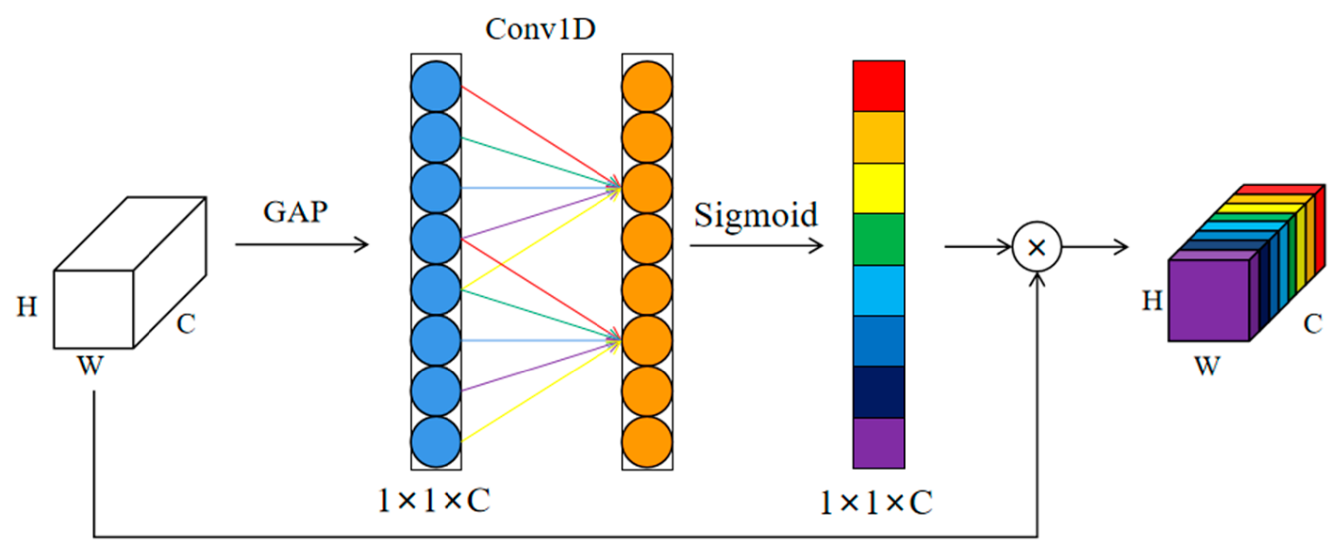
Inspired by pioneering work, this study aims to design a spatial–temporal feature attention network (STFAN). The proposed model can extract deep spatial–temporal fusion features, enabling the detection of different fault modes. The proposed model has the following features: (i) In the proposed model, an efficient convolutional attention network (ECA) is introduced to adaptively capture the dynamic correlation of spatial variables. (ii) The extraction of spatial features among variables in the original data relies on the CNN and ECA models. The global feature extraction of each variable relies on the LSTM model. (iii) The two types of features are integrated through the weighting of the softmax layer or the voting mechanism. The spatial features of the CNN can be input as the initial state of LSTM, providing a spatial prior for sequence modeling. The main innovative contributions of this work can be summarized as follows:

(1)

To address the spatial and temporal correlation of fault feature data, a network model capable of simultaneously extracting spatial–temporal features has been proposed. Multiple convolutional layers can expand the range of feature extraction, enabling better extraction of spatial dimension features. The addition of BiLSTM allows the model to consider both past and future contexts, enhancing its ability to understand and capture complex temporal dependencies. This model can better represent features, improving the model performance and generalization ability.

(2)

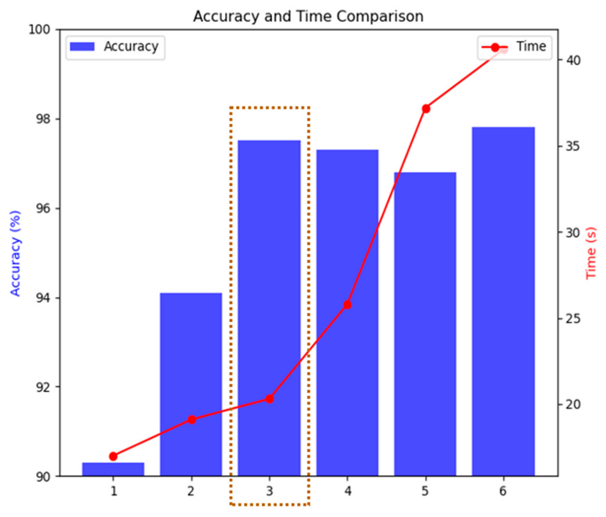
Through the adaptive feature selection mechanism of the ECA module, the model can more effectively capture key features while suppressing noise interference, and simultaneously enhance its ability to understand the global contextual information of sequential data. This approach has achieved significant performance improvements across multiple tasks and demonstrated high-precision stability in repeated experiments, reducing the model’s sensitivity to random initialization.

(3)

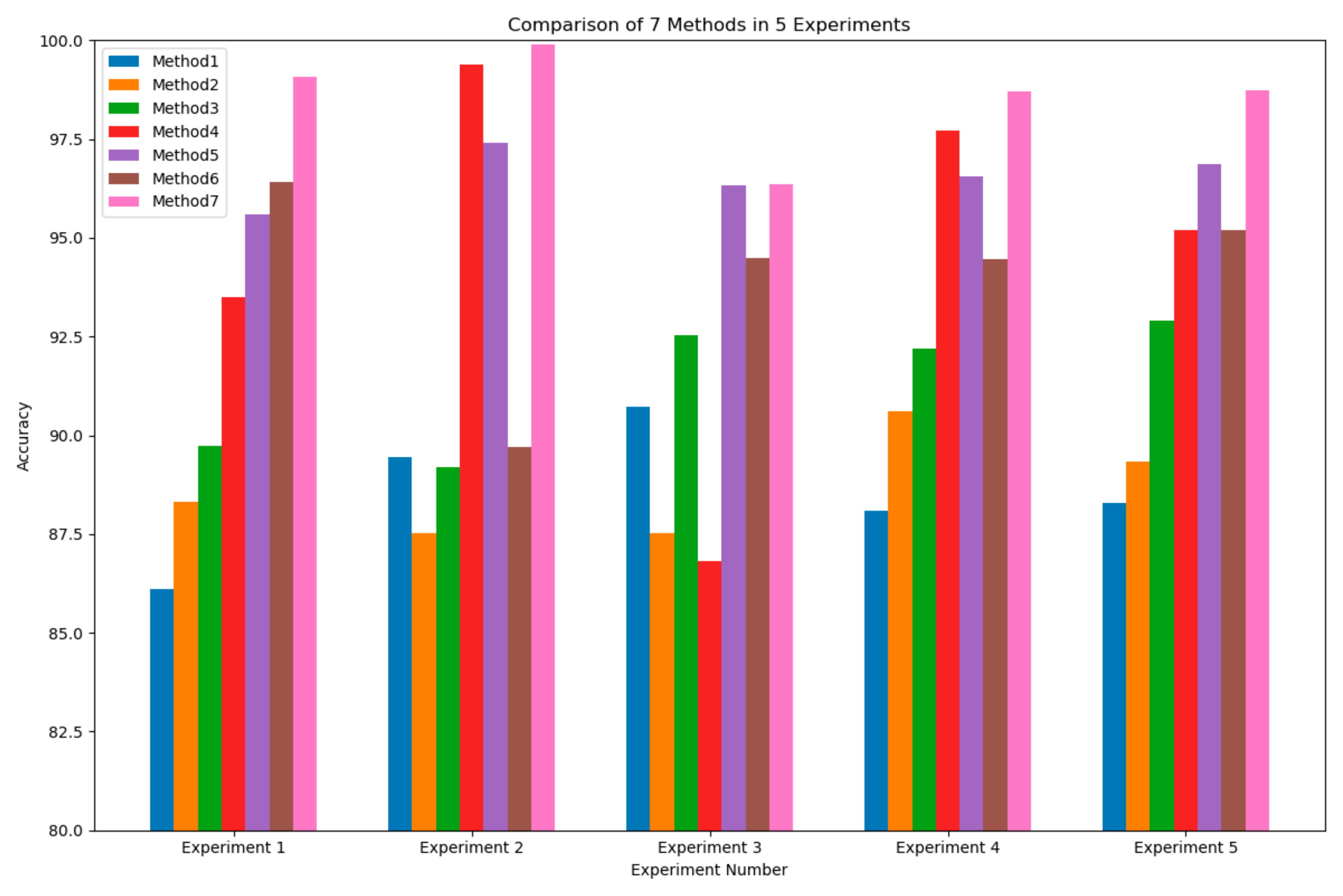
The proposed model method was applied in the field of fault diagnosis of airborne electronic systems. Experimental comparisons were made between the STFAN and BP, SVM, RNN, LSTM, and the proposed method showed significantly better performance in accuracy and stability than the others.

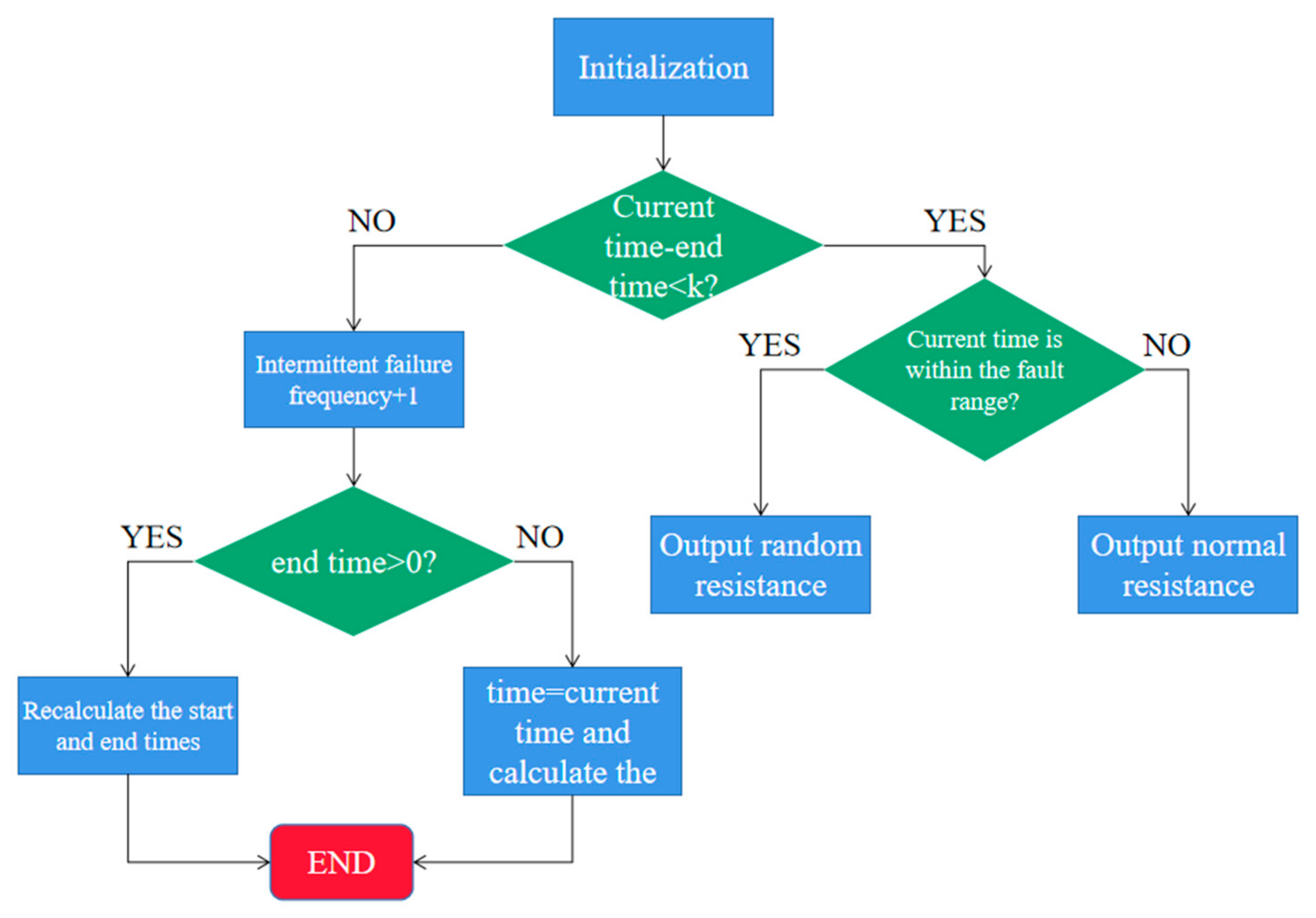
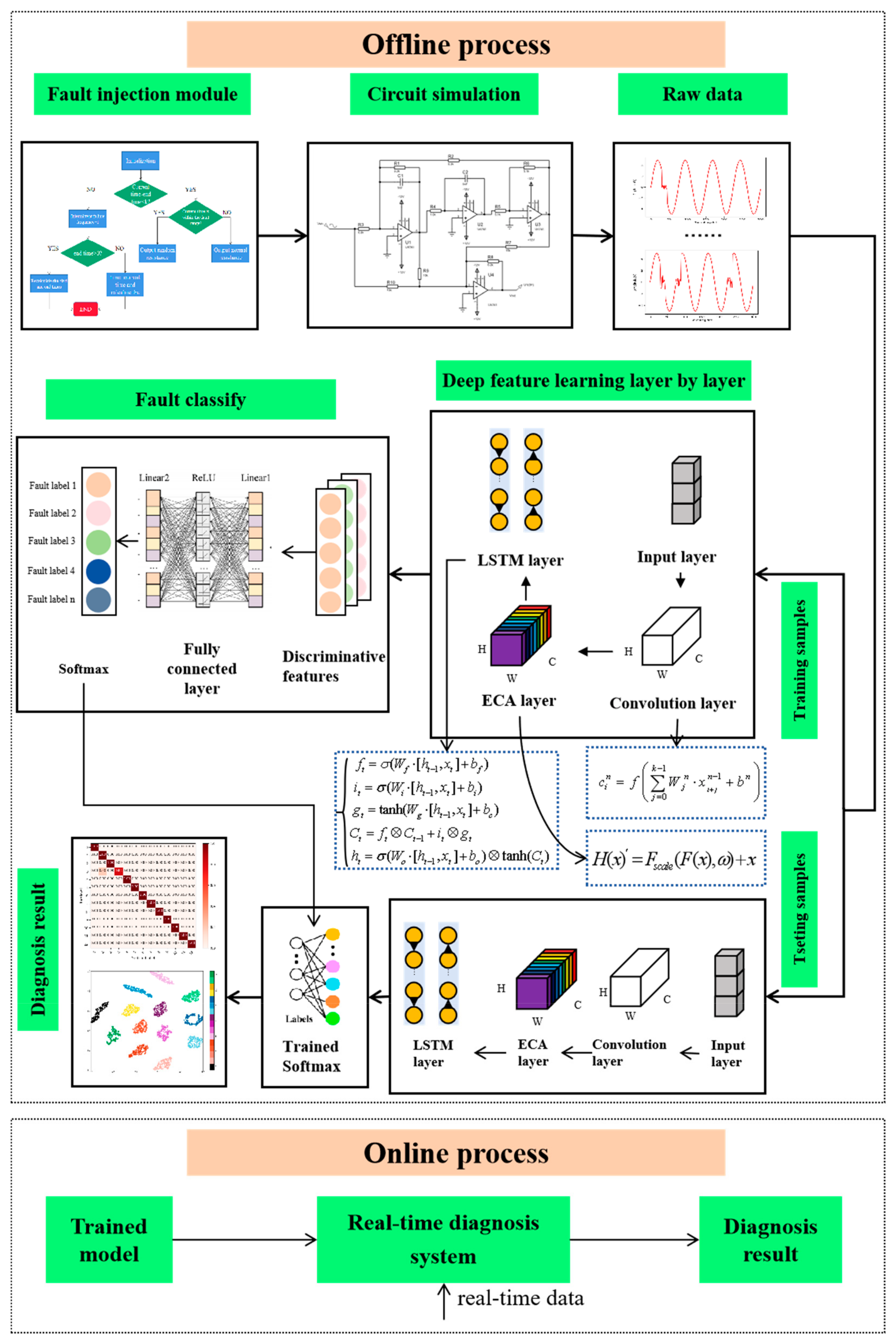
This study consists of the following main sections. Section 2 introduces the related work, including the ECA-ResNet and LSTM; Section 3 introduces the spatial feature extraction model and the temporal feature extraction model, and establishes the STFAN model; Section 4 proposes a fault injection module and provides an overall diagnostic framework; Section 5 experimentally validates the superiority of the proposed method; and this work is summarized in Section 6.

2. Theoretical Background

Related work for fault diagnosis is briefly introduced, including efficient channel attention based on residual network (ECA-ResNet) and LSTM.

2.1. ECA-ResNet

Considering the unequal contribution of extracted features, an attention mechanism is incorporated to prioritize discriminative features while suppressing redundant ones. A Squeeze-and-Excitation Network (SENet), as one of the classic implementations to enhance the performance of convolutional neural networks by introducing a channel attention mechanism, makes the network more flexible in processing the features of different channels and greatly improves the performance of the network. In an SENet, channel attention is achieved through SE blocks. The core idea of SE blocks is to give each channel attention weighting, giving the network more flexibility to focus on the importance of different channels. Specifically, an SE block includes three steps: squeeze, excitation, and scale, where the activation part implements channel attention.

With the continuous improvement in SE attention and the deepening of the deep learning network model, problems such as a large number of parameters, high model complexity, and large amount of computation come along. In addition, the squeezing operation of SE will reduce the prediction performance of channel attention. To address the above problems, Wang et al. proposed an efficient channel attention (ECA) mechanism based on SE attention improvement in 2020 [10]; the structure of the ECA is shown in Figure 1. An efficient channel attention module is proposed, which can improve the performance of the network without increasing the computational cost. The module can be integrated into existing convolutional neural networks to improve their performance.

The ECA module proposes a method for inter-channel interaction to address the dimension reduction issue caused by the SE (Squeeze-and-Excitation) attention mechanism’s squeeze operation. In the ECA module, the input features undergo global average pooling (GAP) to compress the spatial dimensions of the feature map to 1 × 1 while keeping the number of channels unchanged, resulting in a 1 × 1 × C feature map. Then, the ECA module considers only one neighboring neuron for subsequent attention prediction.

Assuming that the C channel attention parameter matrix that k neurons need to learn is denoted as w, the equation is as Equation (1).

$$\left.W_k=\left[\begin{array}{cccccccc}{w}^{1,1}& \cdots & w^{1,k}& 0& 0& \cdots & \cdots & 0\\ 0& w^{2,2}& \cdots & w^{2,k+1}& 0& \cdots & \cdots & 0\\ ⋮& ⋮& ⋮& ⋮& \ddots & ⋮& ⋮& ⋮\\ 0& \cdots & 0& 0& \cdots & w^{C,C-k+1}& \cdots & w^{C,C}\end{array}\right.\right]$$

(1)

The calculation formula for the weight (w_i) of neuron (y_i) is as Equation (2).

$$w_i=\sigma ({\displaystyle \sum _{j=1}^k{w}^j}{y}_i^j),y_i^j\in {\Omega }_i^k$$

(2)

However, the linear function has a limited capacity to express complex relationships. Exponential functions are often used to handle such non-linear mapping relationships. The expression is as Equation (3).

$$C=2^{\left({\gamma }^{n}k-b\right)}$$

(3)

If the number of channels is C, the expression for k can be inferred as Equation (4).

$$k=\psi (C)={\left|{\displaystyle \frac{{\log }_2(C)}{\gamma }}+{\displaystyle \frac{b}{\gamma }}\right|}_{odd}$$

(4)

Then, using a 1D convolution with kernel size k, calculate the channel weights to capture the interdependencies between channels. The formula for 1D convolution is as follows:

$$\omega =\sigma (C_1{D}_k(y))$$

(5)

where w is the channel weight; σ is the Sigmoid function; C₁D is the 1D convolution; y is the result after global average pooling; and k is the kernel size.

The ECA_ResNet network combines ResNet and ECA. It first introduces non-linear mapping, feature transformation, and adaptive adjustment to the network through Conv1D + BN + ReLU. Then, it gradually extracts features through two convolutional layers. After ECA, the original input features are dot-produced with the channel weights to obtain features with channel attention. The improved residual operation formula is as Equation (6).

$$H{(x)}^{\prime }=F_{scale}(F(x),\omega )+x$$

(6)

where F(x) is the residual mapping feature, w is the channel weight, and x is the identity mapping.

Overall, the ECA-ResNet has three advantages:

(1)

Dynamic weight allocation of channel attention.

(2)

Enhancement effect of the residual network.

(3)

Efficiency brought by the lightweight design.

2.2. LSTM

The time series features of raw data typically exhibit strong temporal correlations and implicit patterns that are difficult to capture solely through convolution operations. Recurrent neural networks (RNNs) are capable of operating on both the output features from the previous time step and the current time step’s data as inputs. Therefore, embedding the output of convolutions sequentially into LSTM networks can establish temporal–spatial correlations in the data. The LSTM structure features a main line structure denoted by red arrows. Within this structure, the input C_t−1 represents the information memorized by the previous neuron. At time t, the neuron dynamically forgets some information and incorporates new information. The updated neuron state is combined with h_t−1 to produce h_t. This output is passed on to the neuron at time t + 1 and deeper layers.

Within a cell unit, as is shown in Figure 2, there are primarily three gates: the forget gate, the input gate, and the output gate. According to the input x_t and the previous hidden state h_t−1, the forget gate decides whether to discard redundant information, while the input gate updates the newly added information. The output gate combines the new state information to obtain the current hidden information of the neuron. The calculation process of the LSTM unit can be summarized as Equations (7)–(11):

$$f_t=\sigma (W_f\cdot [h_{t-1},x_t]+b_f)$$

(7)

$$i_t=\sigma (W_i\cdot [h_{t-1},x_t]+b_i)$$

(8)

$$g_t=\tanh (W_g\cdot [h_{t-1},x_t]+b_c)$$

(9)

$$C_t=f_t\otimes C_{t-1}+i_t\otimes g_t$$

(10)

$$h_t=\sigma (W_o\cdot [h_{t-1},x_t]+b_o)\otimes \tanh (C_t)$$

(11)

where W_f and b_f represent the weight matrix and bias vector, respectively; $\sigma$ represents the sigmoid activation function; $\otimes$ denotes the Hadamard product; and the operation ft denotes the element-wise multiplication with the previous neuron’s state value. When the resulting value is 1, no information is forgotten, and when the value is 0, all information is forgotten.

3. Methodology

In this section, the spatial feature extraction model and the temporal feature extraction model are introduced, respectively. Among them, the spatial feature extraction adopts the ECA-ResNet network model embedded with multiple convolutional layers, and the temporal feature extraction adopts BiLSTM. Finally, the complete STFAN network structure is established.

3.1. Spatial Feature Extraction

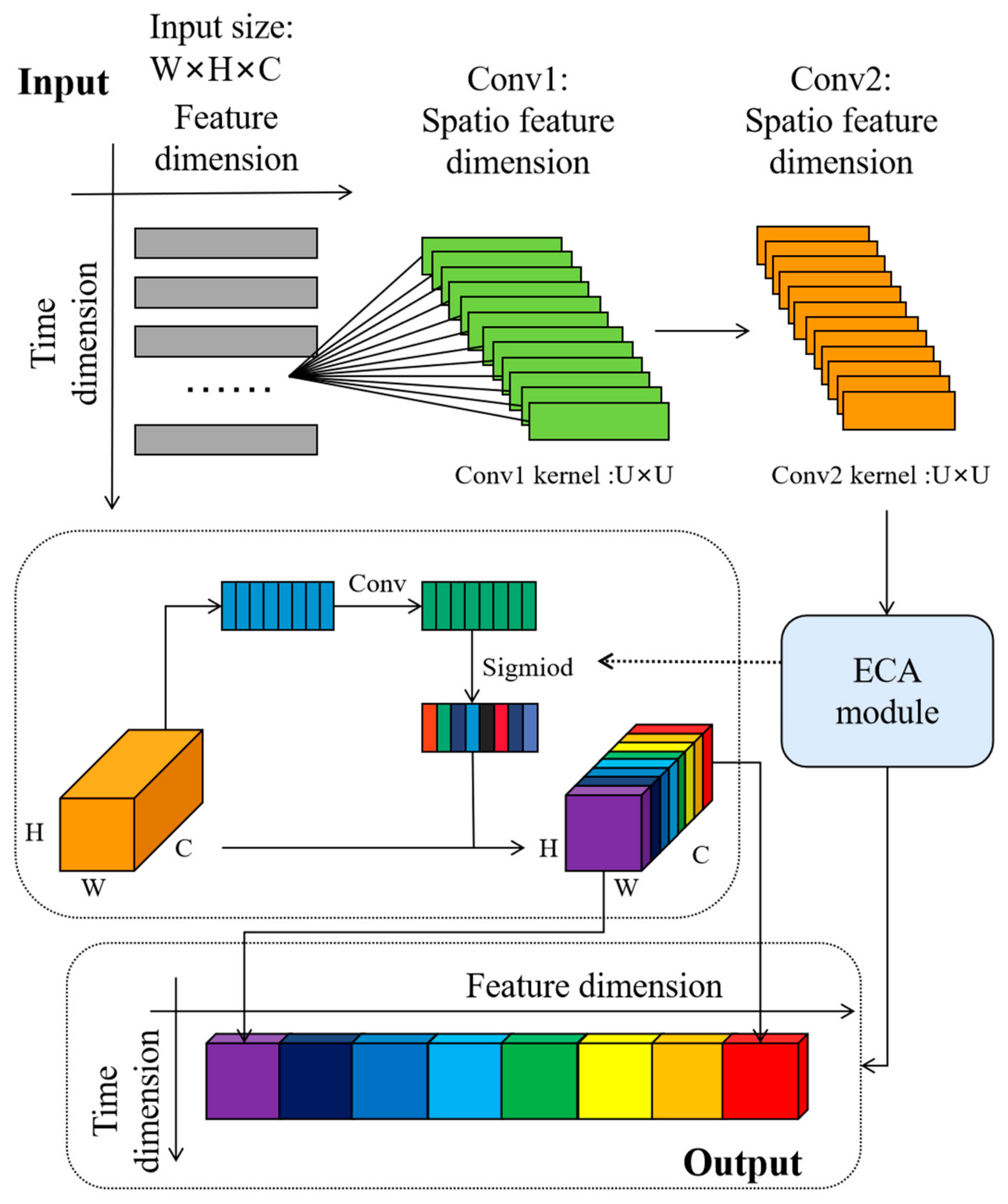
To obtain a comprehension of fault information, multiple convolutions for feature extraction are introduced. Convolution possesses outstanding capabilities in extracting local features. It can gradually obtain higher-level feature representations through multiple convolution layers. These advanced feature representations can help LSTM better understand abstract features within input sequences, which consequently enhances the performance. Additionally, it effectively reduces the model’s parameter count through parameter sharing and exploits local receptive fields to model the local structures of the data efficiently. This approach mitigates the risk of overfitting and enhances the model’s generalization ability.

The purpose of multiple convolutions is to automatically learn and extract spatial features from the data. By using a sliding window approach, local feature extraction is performed on the input data. This process involves element-wise multiplication and summation operations between the convolution kernels and input data, effectively capturing local structures and patterns within the input data. The multiple convolutions can be illustrated as Equation (12).

$$c_i^n=f\left({\displaystyle \sum _{j=0}^{k-1}{W}_j^n}\cdot x_{i+j}^{n-1}+b^n\right)$$

(12)

The structure of the proposed spatial feature dimension model is shown in Figure 3.

3.2. Temporal Feature Extraction

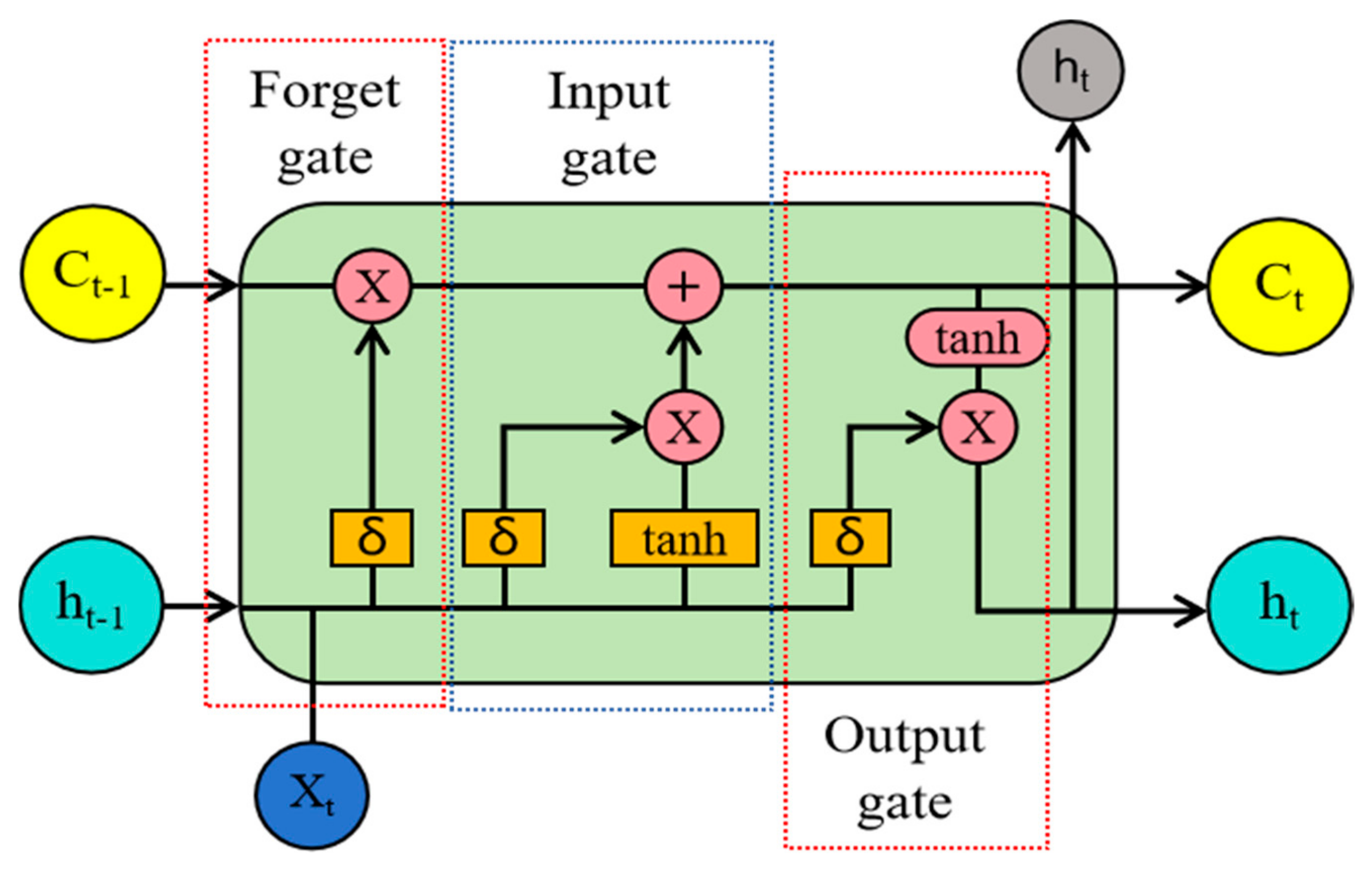
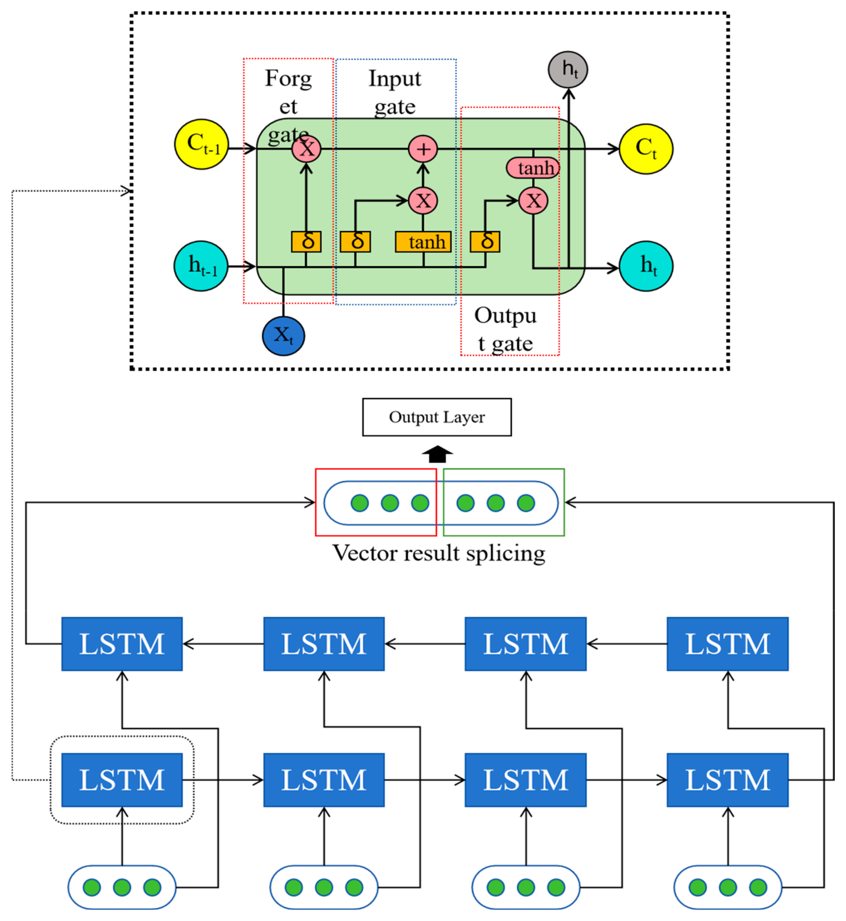
BiLSTM consists of two LSTM units operating in opposite directions. LSTM introduces the concepts of gate units and cell state. The input gate controls the input information from the previous layer, while the forget gate manages the memory information from the previous time step. The training process of the BiLSTM network includes two steps: forward propagation and backward propagation. Forward propagation processes the input from the beginning to the end of the sequence, while backward propagation processes the input in reverse. This bidirectional approach allows the model to consider both past and future states, enhancing its understanding and ability to capture complex temporal dependencies. During the training process, the network parameters are iteratively adjusted through optimization algorithms to improve its performance in handling sequential data.

As shown in Figure 4, a single-layer BiLSTM consists of two LSTM units, one processing the input sequence in the forward direction, and the other processing the sequence in the reverse direction. After processing is complete, the outputs of the two LSTMs are concatenated. The final BiLSTM output is obtained only after computing all time steps. The forward LSTM produces a result vector after four time steps, while the backward LSTM also produces another result after four time steps. These two result vectors are concatenated to yield the final output of BiLSTM.

The proposed BiLSTM model is able to learn temporal sequences and extract global features. The BiLSTM model preserves patterns of temporal changes through its cell state, making it capable of learning long-term information. By inputting the subsequence image feature data outputted by ECA and the original image data into BiLSTM for global learning, deep spatial–temporal fusion features can be extracted.

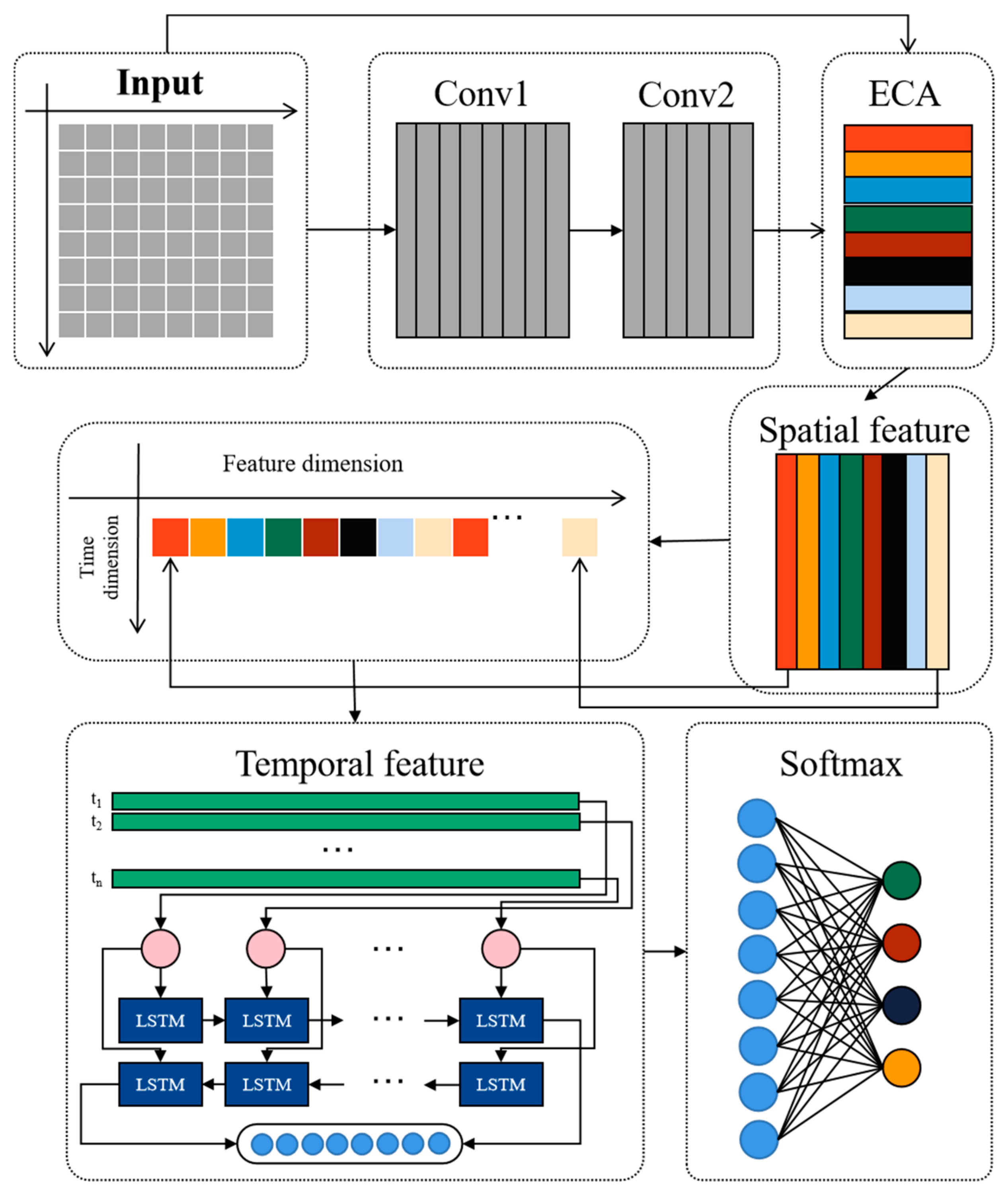
3.3. STFAN Method

In this paper, a novel method called spatial–temporal feature attention network (STFAN) is proposed. This method includes three parts: multiple convolutions, the ECA module, and BiLSTM module. Spatial features (CNN/ECA) represent the local structural correlations of signals, while temporal features (BiLSTM) capture the dynamic evolution patterns of sequences. These two types of features have an inherent complementarity in the information dimension, which conforms to the principle of maximum entropy. Moreover, the hierarchical feature extraction of the CNN and the temporal dependence modeling of LSTM form a multi-scale synergy. The specific fusion principle is as follows: Firstly, the feature space is expanded through tensor concatenation. Then, gating units are introduced to dynamically adjust the contribution degrees of spatial and temporal features. Finally, the two types of features are integrated through the weighting of the softmax layer or the voting mechanism. The spatial features of the CNN can be input as the initial state of LSTM, providing a spatial prior for sequence modeling. On the other hand, the temporal context of BiLSTM can modulate the feature extraction process of the CNN. The spatial features are expanded in the temporal dimension of LSTM to form a spatio-temporal joint feature tensor. The temporal features are compressed into a spatial feature enhancement vector through operations such as global average pooling, achieving the maximization of the mutual information between spatial and temporal features.

This model is a deep learning model for fault diagnosis, designed to handle data with both temporal and spatial features. Firstly, the model uses convolution to process the original one-dimensional data, achieving dimensionality expansion and local feature extraction. Then, the model utilizes an ECA module based on residual networks to focus on important features, enhancing the model’s perception of specific characteristics. Next, the model uses BiLSTM to focus on temporal features, capturing the temporal correlations in the data. Finally, the model uses softmax for classification, categorizing the data into different classes for fault diagnosis. The model combines the processing of temporal and spatial features to comprehensively analyze and diagnose faults. The structure of the proposed STFAN method is shown in Figure 5.

This approach has better automatic feature extraction capability compared to traditional feature engineering methods. Traditional methods often require the manual selection and extraction of features, which may be limited when dealing with complex data. Using deep learning models, especially models that combine a CNN and BiLSTM, can automatically learn and extract important features from the data, thereby improving the accuracy and efficiency of fault diagnosis.

Compared to a single model, the method that combines multiple models can comprehensively capture features in the data. A CNN is suitable for extracting local features, ECA enhances the correlation between features, and BiLSTM can capture long-term dependencies in time series data. Therefore, this multi-model approach can more effectively utilize the diversity of data and improve the accuracy of fault diagnosis.

Compared to other deep learning models, ECA has a better channel attention mechanism, which can better explore the features in the data. Traditional attention mechanisms may only focus on partial channels’ information, while ECA can simultaneously consider all channels, thus having a more comprehensive understanding of the features and improving the model’s accuracy.

The classifier consists of two feed-forward multi-layer perception layers and a softmax function. The data with temporal–spatial correlated features, extracted and fused through LSTM, will be fed into the classifier for final pattern recognition. The softmax can be represented as Equation (13).

$$\mathrm{softmax}(z_i)={\displaystyle \frac{e^{z_i}}{{\displaystyle \sum _{j=1}^N{e}^{z_j}}}}$$

(13)

4. The Proposed Fault Diagnosis Method

In this section, a fault diagnosis method is proposed with the network model proposed above. A fault injection module is introduced first, then the fault diagnosis framework and steps are given.

4.1. Fault Injection Module

Based on the principles of fault generation, a novel fault injection algorithm has been designed. This algorithm is capable of generating diverse fault data by simulating various fault modes, thereby testing the performance of the proposed method under abnormal conditions and evaluating its fault diagnosis capabilities. The fault injection algorithm is shown in Figure 6.

The specific steps are as follows:

(1)

Initialization: At the beginning of the algorithm, initialization is carried out. To track the state of the fault injection, persistent variables are introduced, including counter, start Time, end Time, num Changes, and last Change Time. Counter is initialized to 0 and is used to count the number of fail-over changes. Start Time and end Time are initialized to 0, and they will be used to determine the time range for each failure change. Num Changes is initialized to a custom value, and last Change Time is initialized to −1.

(2)

Condition check: At the beginning of each time step, the algorithm will check whether the condition of fault change is met. This condition is to check whether the time interval between the current time and the last fault change exceeds k seconds. If the time interval meets the condition, a fault change is triggered.

(3)

Fault change trigger: If the time interval meets the condition, the counter will increment, indicating that a fault change has been triggered. If the counter is still less than or equal to the preset num Changes of the total number of failures, then continue to the next step; otherwise, no more failures are triggered.

(4)

Random parameter generation: Generate a random time for start, current time plus a random value of the specified interval generated randomly to simulate the fault from the current time. Generate random duration end Time; this time will be a starting Time plus a randomly generated random value between the specified interval, indicating that the fault will end at this time. Generate a random target resistance value at specified time intervals to simulate random fluctuations in resistance.

(5)

Resistance generation: During the fault change, a resistance value will be output, which is randomly generated within the set range. This resistance value simulates the resistance change caused by faults in the circuit.

(6)

End the fault change: Once the current time is greater than or equal to the end Time, it means that the duration of the fault change has ended, and the algorithm sets the resistance value to normal. This means that the fault has ended and the road returns to the normal state.

This fault injection method involves continuously adjusting the values of various variable components to simulate different faults. Its advantages include the following: high flexibility, high precision, low cost, and wide applicability. It can flexibly simulate different types and severities of faults without modifying the hardware circuit. By adjusting the values of variable components, the occurrence time, duration, and impact range of faults can be precisely controlled, allowing for more accurate assessment of system performance and stability. Compared to using special fault simulation equipment, this method requires lower costs as it only requires common variable components.

4.2. Fault Diagnosis Framework

The proposed model follows a two-stage deployment pipeline. The training phase occurs once on a high-performance workstation and the optimized model is deployed to embedded systems for real-time use, requiring zero retraining. The framework of the STFAN is presented in Figure 7. The general procedures are summarized as follows:

• Step 1: Data preparation phase. Design the circuit to be diagnosed and simulate it. Design different circuits according to actual needs and collect the required data. It is important to check whether the dimensions of the collected data match those of the model. If they are different, appropriate methods should be used for data preprocessing.
• Step 2: Fault injection phase. Use the previously mentioned fault injection method to inject different faults and collect the raw signals obtained. Firstly, select the fault type. Then, determine the injection timing. Decide when and how often to inject the fault, such as injecting the fault at a specific time interval with a certain frequency. Lastly, inject the fault. Inject the fault signal into the original data at the specified timing and frequency, simulating different faults in real systems. Use simulation circuits to collect raw data, including samples of different fault types. Divide the raw data into training samples and testing samples. For example, 70 percent of the whole samples are used for training and the last for testing.
• Step 3: Feature extraction phase. Input the training data into the network for training. Firstly, use multiple convolutions to extract spatial features, then use an ECA-ResNet-based method to assign different attention weights to different features, and finally use BiLSTM to extract temporal features, capturing fault patterns in the time domain. Additionally, using attention mechanisms to enhance the model’s focus on different time steps may enhance the extraction capabilities.
• Step 4: Feature fusion and classification phase. Combine spatial and temporal features to obtain a complete feature representation and use a softmax classifier to classify the feature representation and identify the fault type.
• Step 5: Result analysis and evaluation phase. Input the test samples into the trained model to verify the performance of the proposed method. Analyze the classifier’s output to determine if it correctly identified the fault type. Calculate performance metrics such as accuracy, recall, etc., to evaluate the algorithm’s performance.

Through these steps, the entire process of fault injection, feature extraction, and diagnosis of faults can be completed.

In addition, the model proposed in this paper can run in real time on the embedded diagnostic system. Since this paper discusses the offline training process of the model, during real-time online diagnosis, the model no longer needs to be trained again. Instead, it only requires inputting data into the model for testing, which can meet the real-time requirements of the system.

5. Experiment

This section describes the experimental setups for the method. Contrast experiments are conducted for assessing the superiority of the proposed STFAN method.

5.1. Experimental Data

5.1.1. Circuit and Fault Setting

The Butterworth filter is linear time-invariant. One of the characteristics of the Butterworth filter is that its phase response is relatively smooth with respect to the change in frequency, especially in the passband with an approximately linear phase. This feature makes Butterworth filters useful in some applications that are sensitive to phase response, such as avoiding signal distortion in signal processing. The higher the series of the Butterworth filter are, the steeper its filtering characteristics are. Filters of higher order can usually provide better frequency selectivity, and at the same time can better counter the noise in the signal and improve the signal-to-noise ratio of the system. In this paper, the high-order Butterworth filter circuit is selected and the simulation model is established with Multisim.

Firstly, a detailed high-pass Butterworth filter circuit model is established, as shown in Figure 8, in which R1, R2, R3, and R4 use variable resistance modules, C1 and C2 are variable capacitance modules, and then the fault injection algorithm is used for fault injection. The variable resistance, capacitor, and fault injection module are combined to simulate the occurrence of a fault. Each component’s parameters are also labeled on the diagram.

By implementing the previously described fault injection methodology, which introduces faults at various frequencies across distinct component locations, twelve distinct fault types were systematically generated for specific components. More details about the twelve conditions are listed in

Table 1. Sample distribution of 13 conditions.

Condition	Number of Faults	Resistance Value Fluctuation Range	Fault Type	Fault Sign
Normal	-	-	NF	NO
R1	[0, 2]	[5%, 8%]	FT	FT1
R1	[3, 5]	[5%, 10%]	FT	FT2
R2	[0, 2]	[5%, 8%]	FT	FT3
R2	[3, 5]	[5%, 10%]	FT	FT4
R3	[0, 2]	[5%, 8%]	FT	FT5
R3	[3, 5]	[5%, 10%]	IF	FT6
R4	[0, 2]	[5%, 8%]	FT	FT7
R4	[3, 5]	[5%, 10%]	FT	FT8
C1	[0, 2]	[5%, 8%]	FT	FT9
C1	[3, 5]	[5%, 10%]	FT	FT10
C2	[0, 2]	[5%, 8%]	FT	FT11
C2	[3, 5]	[5%, 10%]	FT	FT12

. The originals of the fault injection are R1, R2, R3, R4, C1, and C2, respectively. There are two types of fault modes, which are normal state and fault state. NF is the signal of the normal state, FT represents different fault degrees of different components, and every fault type contains two conditions: the number of faults and the fluctuation range of resistance (capacitance) value; the fault value is a range, which will return to the normal state after a short fault, where the resistance fluctuation range is ±10% and the capacitance fluctuation range is ±10%. For example, FT1 corresponds to zero to two times of resistance changes for R1 and each represents a change in resistance from 5% to 8%.

5.1.2. Data Collection

Collect raw data using the above simulation circuit, with each fault type containing 1000 samples, each sampled for 2 s, consisting of 2000 data points. Figure 9 shows the raw data samples of the twelve conditions. To avoid the randomness of the diagnostic results, we used 700 samples for training in each case, and the remaining 300 samples for testing. The labels of each condition are shown in

Table 2. Labels of each condition.

Fault Sign	The Number of Trainings	Testing Samples	Label
NO	700	300	0
FT1	700	300	1
FT2	700	300	2
FT3	700	300	3
FT4	700	300	4
FT5	700	300	5
FT6	700	300	6
FT7	700	300	7
FT8	700	300	8
FT9	700	300	9
FT10	700	300	10
FT11	700	300	11
FT12	700	300	12

.

5.2. Comparison Results and Discussion

5.2.1. Parameter Settings

In order to demonstrate the effectiveness and advantages of the proposed method, a back propagation neural network (BPNN), support vector machine (SVM), and recurrent neural network (RNN) are adopted for comparison. In addition, a method that is named incomplete STFAN (ISTFAN) by removing the ECA module from the proposed method is used for comparison with the original method to determine whether the addition of the ECA module can improve the performance of the model.

In the STFAN, the CNN is used to extract initial spatial features from the input data, and these features often contain a large amount of redundant information. The ECA residual network module, through its channel attention mechanism, can selectively choose important channel features, reduce redundant information, and maximize the mutual information between the latent representation and the target labels at the same time. By processing the spatial features with the CNN-ECA residual network, the information entropy of the features can be reduced, making the features more orderly and discriminative. When processing time series data, BiLSTM can also reduce the information uncertainty in the time dimension by learning the temporal dependencies in the sequence, thereby improving the entire system’s ability to understand and represent the data. BiLSTM can effectively control the flow of information by introducing the gating mechanism, ensuring that the dynamic changes in the hidden states have stability and convergence in long sequences. The parameters of the STFAN model are all selected and experimentally verified according to the above principles.

In this study, the main parameters of the proposed method are available in

Table 3. Parameters of the proposed method for fault diagnosis.

Description	Value
Number of convolutional layers	2
The number of convolutional kernels of the first layer	32
The number of convolutional kernels of the second layer	64
The number of channels in ECA	64
Number of modules in ECA_Resnet	3
Number of layers in BiLSTM	3
The units of the first hidden layer	32
The units of the second hidden layer	64
The units of the third hidden layer	64
Number of iterations	100
Batch size	32

. The original data obtained from simulations are first input into the convolutional layers to obtain feature maps for the ECA input. There are two convolutional layers, each with 32 and 64 kernels, respectively, and the kernel size is 3. The resulting feature maps are then input into the ECA-ResNet for training. The ECA module contains 64 channels and three attention modules. The BiLSTM layer consists of an input layer and three hidden layers with hidden unit sizes of 32, 64, and 64. The model is trained for 100 epochs with a batch size of 32.

The main parameters of other methods are described as follows.

• Method 1 (BPNN): The dimension of its input layer is 2000, which is determined by the number of original features. The number of hidden layers is set to 500 according to the empirical rule. The ReLU function is used for activation to prevent gradient vanishing, and the dropout is set to 0.3 to prevent overfitting. The dimension of the output layer is 13, corresponding to 13 types of faults. The training will be stopped when the loss of the validation set does not decrease for five consecutive generations, and the number of iterations is determined to be 100.
• Method 2 (SVM): Choosing the RBF kernel function can automatically handle the problem of non-linearly separable data and avoid the curse of dimensionality of the polynomial kernel. A relatively large value of gamma, which is 32, is selected. This value has a tendency towards overfitting but is suitable for the scenario in this paper where there is a high correlation between features. A relatively small value of C, which is 0.32, is chosen. In this way, the penalty for wrong samples can be reduced, and the generalization ability of the model can be improved.
• Method 3 (RNN): Choosing 128 units in the hidden layer can balance the sequence modeling ability and computational complexity. The tanh activation function is selected to adapt to the characteristics of time series data. The Adam optimizer is chosen, which combines momentum and an adaptive learning rate. LSTM is not adopted due to the limitation of computational resources.
• Method 4 (GAN): There are six residual blocks, which can balance the generation ability and computational efficiency, making it suitable for the generation of fault data. The discriminator has an architecture of 70 × 70. The local discriminator enhances the authenticity of the generated details and avoids the mode collapse caused by the global discriminator. The cycle consistency loss is set to 10, and the Adam optimizer is adopted.
• Method 5 (Transformer): The number of attention heads is set to eight, which are divided into four spatial heads and four temporal heads to adapt to the spatio-temporal characteristics of the fault signals. The learnable 1D position encoding is used for position encoding, which retains the sequential information of the time series and is superior to the fixed encoding in terms of flexibility. The AdamW optimizer is adopted to avoid the conflict of weight decay.
• Method 6 (ISTFAN): remove the ECA layer from the original model and keep all parameters of other layers the same.

5.2.2. Comparison Result

Five trials are performed to show the stability of the proposed method. Figure 10 shows the detailed results in each trial, and the average testing accuracies are listed in

Table 4. Diagnosis result of different methods.

Methods	Diagnosis Result	Accuracy	Standard Deviation	Time (s)
Method 1 (BPNN)	17,492/19,500	89.70%	1.58	25.6
Method 2 (SVM)	17,573/19,500	90.12%	2.66	22.6
Method 3 (RNN)	18,067/19,500	92.65%	2.31	31.5
Method 4 (GAN)	18,375/19,500	94.23%	5.03	40.5
Method 5 (Transformer)	18,853/19,500	96.68%	2.23	55.0
Method 6 (ISTFAN)	18,568/19,500	95.22%	3.35	40.3
Method 7 (the proposed method)	19,044/19,500	97.66%	1.22	44.2

. From Figure 10, the testing accuracy of the proposed method in each trial is, respectively, 97.3% (3795/3900), 96.8% (3775/3900), 98.3% (3834/3900), 98.1% (3826/3900), and 97.8% (3814/3900). It can be observed from Table 3 that the average accuracy of the proposed method is 97.66% (19,044/19,500), and it is much higher than the BPNN, SVM, RNN, and ISTFAN, which are 89.70% (17,492/19,500), 91.12% (17,573/19,500), 92.65% (18,067/19,500), and 95.22% (18,568/19,500), respectively. In addition, the standard deviation of the proposed method is 1.22, which is much smaller than other methods (1.58, 2.66, 2.31, 3.35). Figure 11 gives the confusion matrix of the proposed method and Figure 12 is the t-Distributed Stochastic Neighbor Embedding (t-SNE) visualization.

From Figure 11, it can be seen that the model mistakenly diagnosed the fault of R2 as the fault of R1. By observing the characteristics of the data of these two faults, it was found that the shapes of the two groups of data were roughly similar, and the difference lay in the position where the fault occurred. The possible reasons for the misjudgment of the model are as follows: Firstly, it may be due to the local perception bias of the convolutional operation. When the fault location spans multiple receptive fields, there is spatial misalignment in feature extraction. Secondly, it may be due to the defect in the position encoding of time series modeling. When the fault location is at the edge of the time window, the loss of contextual information may occur due to sequence truncation. It may also be because of the loss of position information during feature fusion. When the current model uses the feature concatenation method to fuse spatial and temporal features, the positional correspondence between spatial features and temporal features has not been established.

By comparison, it can be clearly concluded that the proposed method achieves higher accuracy and better stability compared to other deep learning algorithms. This is because the diagnostic performance of the BPNN, SVM, and RNN largely depends on manual feature extraction. After designing some new features or selecting the most sensitive features from the original feature set, their test accuracy may be further improved. However, this is a very time-consuming and labor-intensive task. The advantage of the proposed method lies in the layered feature learning process, which can automatically capture useful representative information from the raw data. Due to the increase in hidden layers, the computational time of current deep learning exceeds that of the BPNN, SVM, and RNN. The results also show that the accuracy rate of the GAN is 94.23%, and the accuracy rate of Transformer is 95.28%. Both are lower than that of the proposed STFAN model. Our fault injection method differs fundamentally from the data-driven approaches of a GAN. It simulates real fault mechanisms through physically constrained component parameter perturbations, while a GAN focus on statistical distribution fitting. Compared to Transformer, the bidirectional gating mechanism of BiLSTM adopted in this paper can capture the temporal correlations more efficiently while maintaining a relatively low computational cost.

The ISTFAN can enhance the extraction of local features to increase the diagnostic accuracy of the model. However, as is shown in Table 4, this model exhibited significant instability in the five experiments. After incorporating ECA, the stability of the model in diagnosis has improved significantly. This is because the introduction of the attention mechanism enhances the model’s focus on features, thereby improving its understanding of the entire time series data. It helps the model capture longer-term dependencies and features, ensuring the stability of accuracy in multiple repeated experiments.

5.3. Ablation Experiment

5.3.1. Effect of Spatial Feature Extraction

The impact of the number of ECA modules on model accuracy is investigated in this section. The convolutional layer is introduced in front of the ECA, the data are initially extracted, and then the attention of the channel is adjusted adaptively through the ECA module, so that the model is more robust to the changes in the input data. In this section, the number of convolutional layers and the number of ECA modules are tested at the same time. The experimental results are shown in

Table 5. Effect of the number of convolutional layers and ECA_Resnet modules on the accuracy.

Number of Convolutional Layers	Number of ECA Modules	Accuracy (%)
1	1	88.3
1	2	89.1
1	3	89.4
1	4	89.2
1	5	90.3
2	1	93.5
2	2	97.1
2	3	97.9
2	4	96.1
2	5	95.3
3	1	93.7
3	2	94.1
3	3	94.9
3	4	97.6
3	5	95.4
4	1	94.2
4	2	96.1
4	3	96.3
4	4	95.4
4	5	95.1

, and the visualization results are shown in Figure 13.

As can be seen from Figure 13, at the beginning, with the increase in the number of network layers and the number of ECA modules, the accuracy maintains an upward trend. However, when the number of convolution layers reaches 2, the accuracy hardly increases or even decreases, resulting in the phenomenon of overfitting. When the number of ECA modules increases to 3, the accuracy rate also reaches the bottleneck and even drops in the case, so the best choice for the number of convolutional layers is 2 and the number of ECA modules is 3.

5.3.2. Effect of Temporal Feature Extraction

In the temporal feature extraction module of the STFAN model, the optimal number of layers and hidden-layer units warrants further investigation. In this section, to begin with, to explore the impact of the number of convolutional kernels on the model’s accuracy, the number of layers was successively set to 1, 2, 3, 4, 5, and 6. Subsequently, the diagnostic accuracy and training time were evaluated. The experimental results are presented in

Table 6. Relationship between the number of layers, accuracy, and training time.

Number of Layers	Accuracy (%)	Training Time (s)
1	90.3	17
2	94.1	19.1
3	97.5	20.3
4	97.3	25.8
5	96.8	37.2
6	97.8	40.6

, and the findings are visualized in Figure 14.

With the increase in layers, the accuracy of the model increases first and then tends to be stable. When the number of layers is 1, the accuracy rate is about 90.3%. The accuracy gradually improves as the number of layers increases, reaching a relatively high level at 3 layers, after which it declines slightly. At the same time, the training time gradually increased with the increase in layers, from 17.0 s with 1 layer to 20.3 s with 3 layers. Thereafter, the training time continued to increase, forming a trade-off with the improvement in accuracy. Considering the accuracy and training time comprehensively, the layer number is finally selected as 3, which can not only improve the accuracy to a certain extent but also maintain a relatively short training time. This choice found a balance point between model performance and computational cost.

After the number of layers is determined, the parameters of the number of hidden-layer units should be determined. Due to the small dataset of faults, the number of hidden-layer units is set to 32, 64, and discussed to evaluate the diagnosis accuracy and training time. The experimental results are shown in

Table 7. Relationship between hidden-layer units, accuracy, and training time.

Hidden-Layer Units	Accuracy Rate (%)	Training Time (s)	Label
32 + 32 + 32	93.5	21.3	1
32 + 32 + 64	96.1	26.4	2
32 + 64 + 64	96.5	27.1	3
64 + 32 + 32	97.6	27.4	4
64 + 32 + 64	97.3	30.6	5
64 + 64 + 64	98.2	37.1	6

and Figure 15.

It can be seen that with the increase in the number of hidden-layer elements, the accuracy of the model will gradually increase, but it will gradually reach a bottleneck, and the training time will also increase greatly. It can also be seen that the increase in the number of elements in the third hidden layer has a relatively obvious effect on the improvement in network accuracy. Balancing the relationship between the accuracy and training time, selecting 32 + 64 + 64 as the hidden-layer parameters yields the best results.

5.3.3. Effect of Batch Size

Batch size refers to the number of samples used in each training iteration. When the dataset is large, a smaller batch size should be used to avoid memory issues. However, reducing the batch size too much can prevent the model from converging. A batch size of 1 is known as online learning, which is prone to being influenced by noisy samples, especially when the dataset is small. With enough samples, the impact of noisy samples on the model can be ignored, but the training time will be longer.

The selection of the batch size plays a crucial role in determining the descent direction. In the case of a small dataset, employing the entire dataset for training can be advantageous. This approach provides a more comprehensive representation of the overall sample, thereby facilitating a more accurate determination of the location of the extremum. Given that the gradients of different weights can exhibit substantial variability, the choice of a global learning rate becomes a formidable challenge.

To investigate its impact, the chosen optimal parameters were used as a basis, and batch sizes of 4, 8, 16, 32, 64, and 128 were employed for training. The training results and times are presented in

Table 8. The relationship between batch size, accuracy, and training time.

Batch Size	Accuracy (%)	Training Time (s)
4	96.03	41
8	96.81	21.5
16	96.79	17.3
32	97.51	17.0
64	86.75	16.3
128	15.20	13.1

. It can be observed that as the batch size increases, the model’s accuracy initially rises and then decreases. Specifically, from a batch size of 4 to 32, the accuracy gradually increases, reaching the peak at 97.51%. However, a sharp decline is observed at batch sizes of 64 and 128. Simultaneously, with an increase in batch size, the training time gradually decreases from 41 s to 13.1 s. The result is shown intuitively in Figure 16.

Taking into account both the accuracy and training time, a batch size of 32 is chosen, achieving a high accuracy of 97.51% with a relatively short training time of 17.0 s.

5.4. Experiment 2

To further verify the accuracy of fault recognition and demonstrate the robustness of the proposed network, a twice-order high-pass filter circuit with four operational amplifiers is established for accuracy validation, as shown in Figure 17.

Capacitors C1 and C2, and resistors R1, R2, and R3 are selected for fault mode setting, totaling five components with 15 states. The fault types include normal state, intermittent faults, and other faults. “Normal” represents the normal state of the signal. The tolerance range for resistors is 5%, and for capacitors, it is 10%. For intermittent faults, the fault value is a range that will recover to the normal state after a transient fault. The fluctuation range for both resistors and capacitors is 10%. The types of faults for the signal are shown in

Table 9. Fault mode.

Fault Tag	Fault Class	Normal Value (NF/KΩ)	Fault Value (NF/KΩ)	Fault Type
F0	Normal	-	-	NF
F1	C1↓	5	4	PF
F2	C1↑	5	5.5	PF
F3	C2↓	5	4	PF
F4	C2↑	5	5.5	PF
F5	R1↓	6.2	5.89	PF
F6	R1↑	6.2	6.51	PF
F7	R2↓	6.2	5.89	PF
F8	R2↑	6.2	6.51	PF
F9	R3↓	6.2	5.89	PF
F10	R3↑	6.2	6.51	PF
F11	$\widetilde{\mathrm{C}1}$	5	[4.3, 5.7]	IF
F12	$\widetilde{\mathrm{C}2}$	5	[4.3, 5.7]	IF
F13	$\widetilde{\mathrm{R}1}$	6.2	[5.58, 6.82]	IF
F14	$\widetilde{\mathrm{R}2}$	6.2	[5.58, 6.82]	IF
F15	$\widetilde{\mathrm{R}3}$	6.2	[5.58, 6.82]	IF

, where NF represents no fault, IF represents intermittent fault, and PF represents permanent fault. The arrows indicate increase or decrease in the components’ parameter value.

The precision of various diagnostic methods under this circuit is shown in Figure 18, with five experiments conducted. Methods 1–3 refer to the BPNN, SVM, and RNN, respectively. The parameters of each method are the same as those in Section 5.2.1. From Figure 16, it can be concluded that the proposed method has a higher accuracy compared to other methods.

The confusion matrix of the proposed method under the twice-order high-pass filter circuit with four operational amplifiers is shown in Figure 19. Except for the misclassification of fault types F1, F3, and F11, where the error rate is approximately 0.18, the proposed method attains an accuracy of over 0.97 for the remaining fault types. The model’s average accuracy stands at 0.96, which is markedly higher than that of other methods.

6. Conclusions

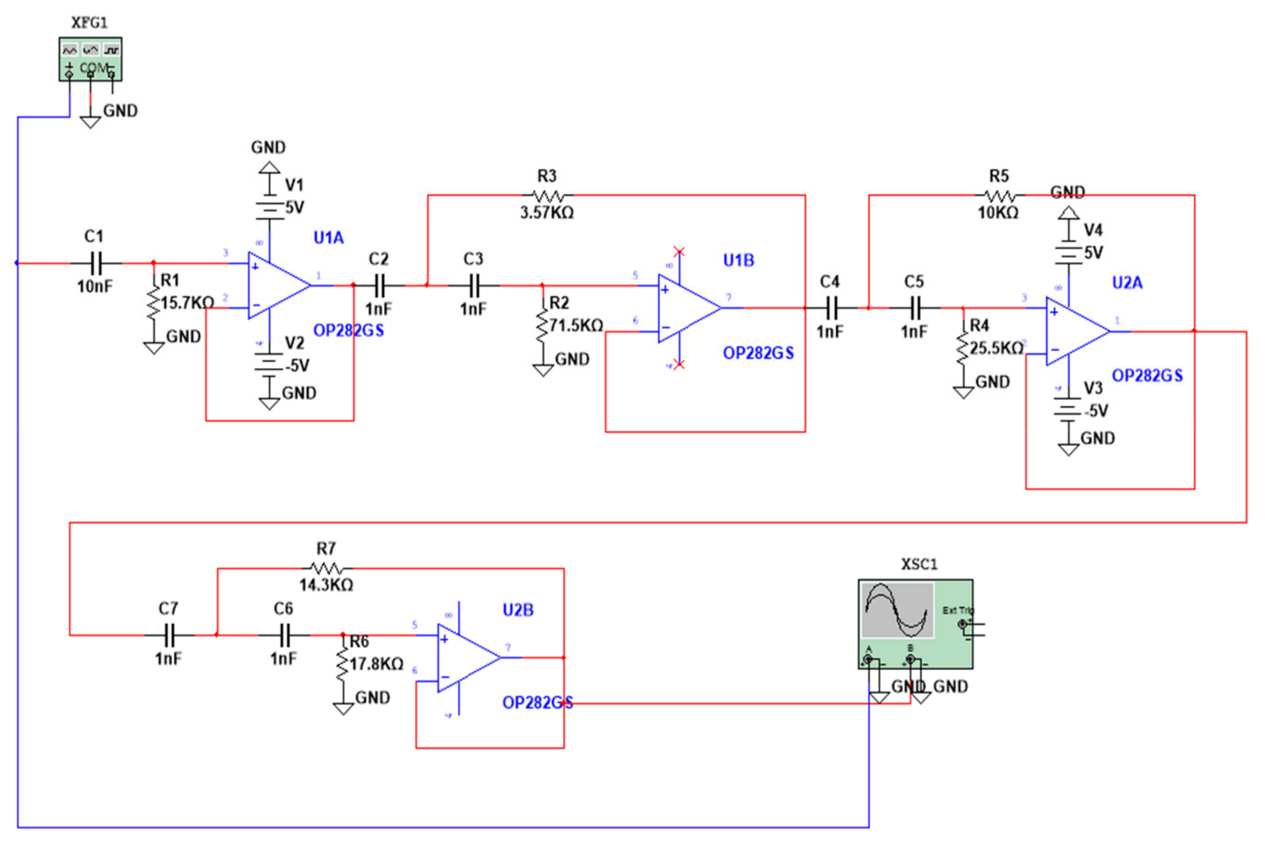
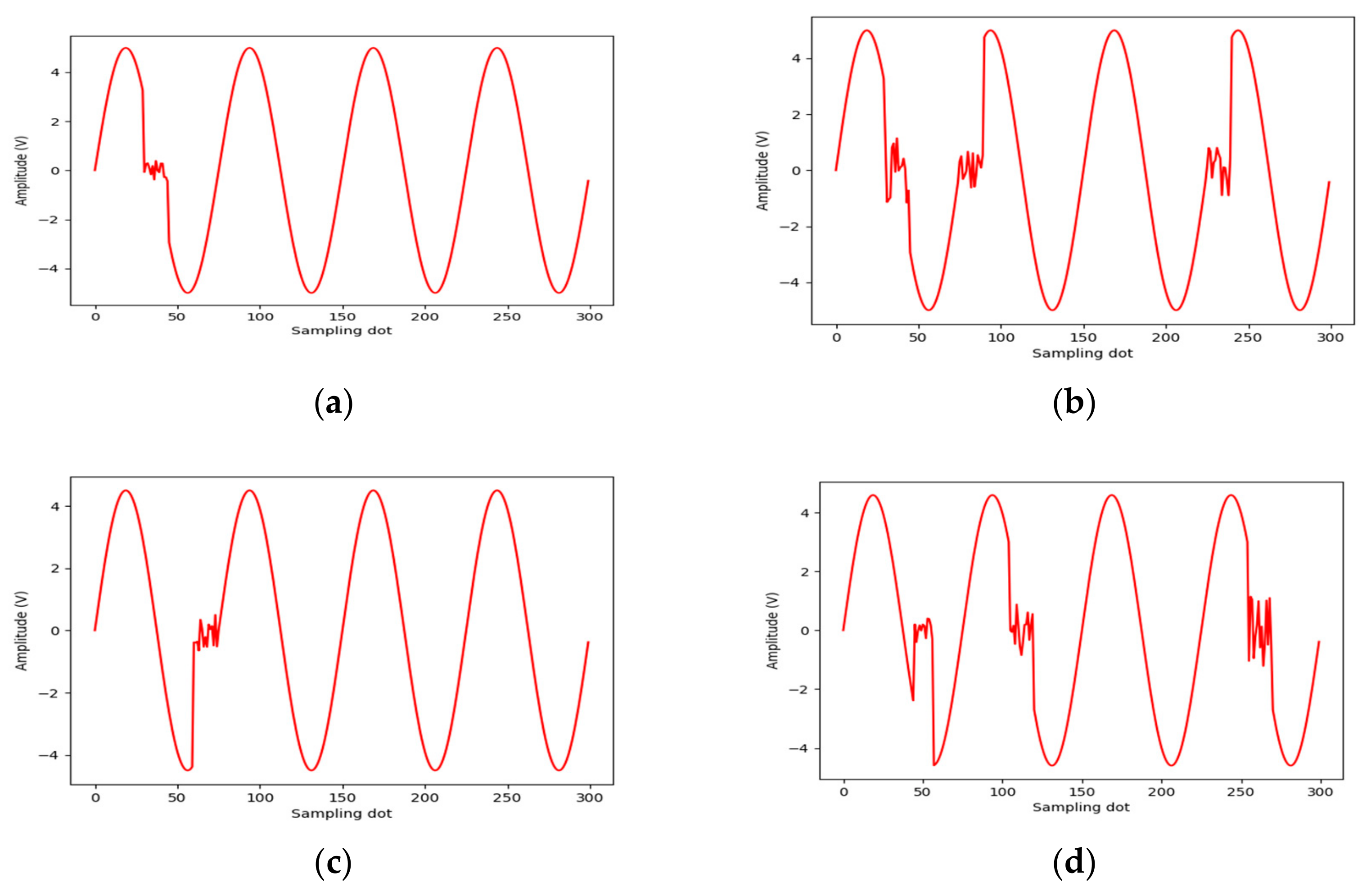
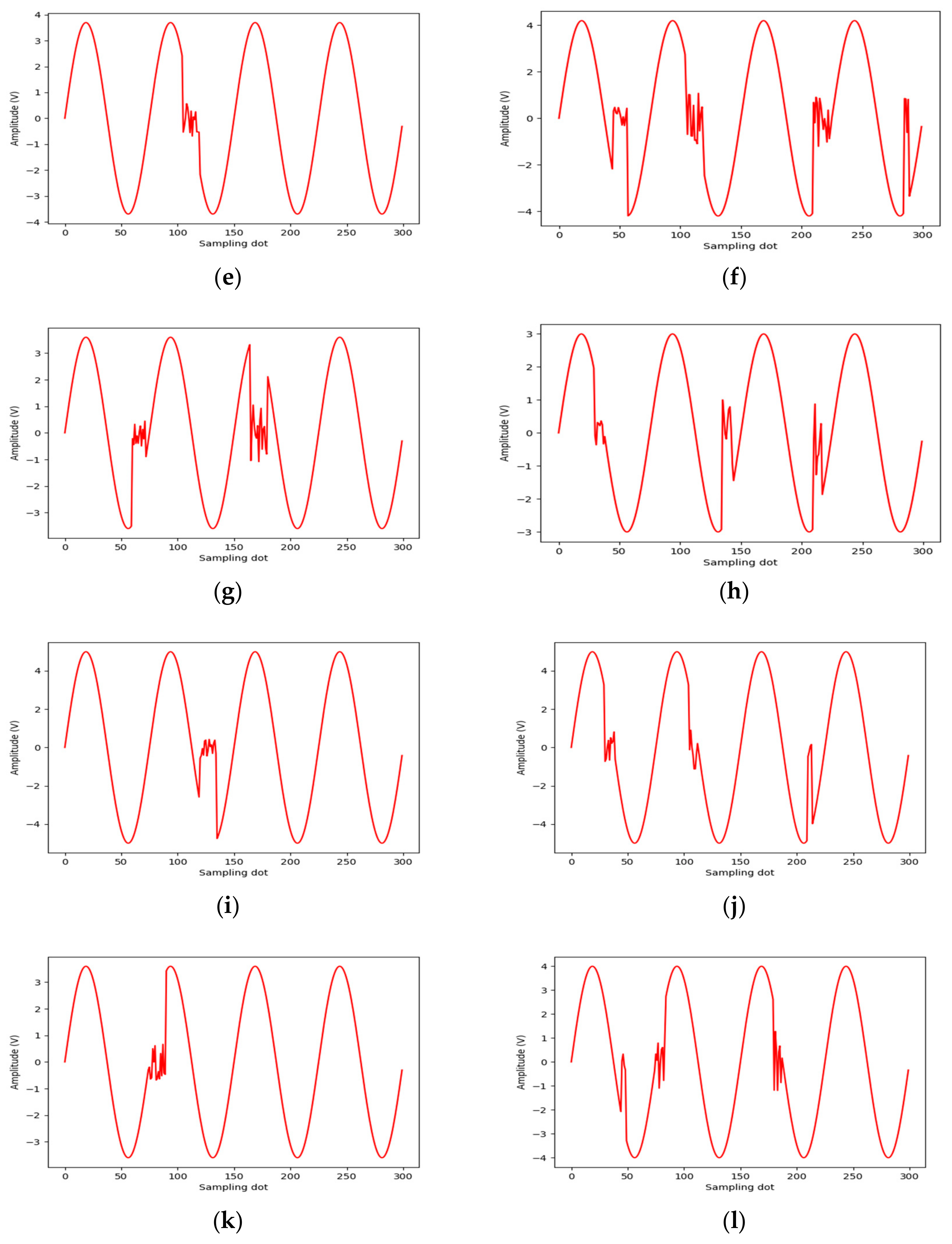
In this paper, a fault diagnosis method based on the STFAN is proposed. Multiple convolution layers are employed due to their capability to extract the most important features from the dataset. At the same time, they can be combined with the ability of LSTM to detect and store long-term dependencies between the extracted data. By extracting features from time and space dimensions, the problems of wide spatial distribution and random occurrence and disappearance time of complex faults can be effectively solved. Moreover, we add the ECA module to the network. The introduction of the attention mechanism enables the network to selectively focus on more important features, which enhances the model’s attention to features, and improves the model’s understanding of the entire time series data. The attention network captures longer-term dependencies and features, and ensures the stability of the accuracy rate of repeated experiments. In addition, we proposed a fault injection strategy to simulate the different operating states of circuit elements, which solves the problem of insufficient fault data. According to the characteristics of faults, a simulation model for the high-order Butterworth circuit was developed. The proposed network is trained and tested on a circuit dataset. Comparative analyses with the results of other deep learning models demonstrate an average accuracy improvement of 7.9% over the BPNN, 7.5% over the SVM, and 5.0% over the RNN in five experiments. Additionally, the stability of the proposed method has significantly improved compared to the ISTFAN. Based on experimental verification, our main conclusions are as follows:

(1)

By using multiple convolutional networks and BiLSTM, the effective extraction of both spatial and temporal features has been achieved.

(2)

By embedding the ECA module, key features are emphasized, enhancing the stability of the model’s accuracy across multiple experiments.

(3)

Experimental results show that the proposed STFAN model effectively extracts the spatial–temporal features of different faults, significantly improving the accuracy of fault diagnosis in analog circuits.

In future work, we plan to apply the proposed method to hardware circuits. Additionally, we have only conducted diagnostic studies on faults; achieving fault prediction in real-world conditions would offer greater practical value. A hardware-in-the-loop (HIL) testbed is currently under development, and we plan to systematically address deployment challenges in physical systems in subsequent work. The simulation results in this study provide a methodological foundation for future real-environment testing.

References

1. Jia, Z.; Liu, Z.; Gan, Y.; Vong, C.M.; Pecht, M. A Deep Forest-Based Fault Diagnosis Scheme for Electronics-Rich Analog Circuit Systems. IEEE Trans. Ind. Electron. 2021, 68, 10087–10096. [Google Scholar] [CrossRef]
2. Cheng, X.; Lv, K.; Liu, G.; Qiu, J. Characteristics of Intermittent Fault in Electrical Connectors Under Vibration Environment. IEEE Trans. Compon. Packag. Manuf. Technol. 2020, 10, 1575–1578. [Google Scholar]
3. Zhou, D.; Zhao, Y.; Wang, Z.; He, X.; Gao, M. Review on Diagnosis Techniques for Intermittent Faults in Dynamic Systems. IEEE Trans. Ind. Electron. 2020, 67, 2337–2347. [Google Scholar]
4. Zhang, K.; Gou, B.; Xiong, W.; Feng, X. An Online Diagnosis Method for Sensor Intermittent Fault Based on Data-Driven Model. IEEE Trans. Power Electron. 2023, 38, 2861–2865. [Google Scholar]
5. Ezhilarasu, C.M.; Skaf, Z.; Jennions, I.K. A Generalised Methodology for the Diagnosis of Aircraft Systems. IEEE Access 2021, 9, 11437–11454. [Google Scholar]
6. Chen, H.; Jiang, B.; Zhang, T.; Lu, N. Data-driven and deep learning-based detection and diagnosis of incipient faults with application to electrical traction systems. Neurocomputing 2020, 396, 429–437. [Google Scholar]
7. Shen, Q.; Lv, K.; Liu, G.; Qiu, J. Dynamic Performance of Electrical Connector Contact Resistance and Intermittent Fault Under Vibration. IEEE Trans. Compon. Packag. Manuf. Technol. 2018, 8, 216–225. [Google Scholar]
8. Li, Y.; Zhou, X.; Li, S. A Intermittent Fault Injection Strategy for Electronic Equipment Health Status Recognition. In Proceedings of the 11th International Conference on Prognostics and System Health Management, Jinan, China, 23–25 October 2020. [Google Scholar]
9. Fang, X.; Qu, J.; Chai, Y.; Liu, B. Adaptive multiscale and dual subnet convolutional auto-encoder for intermittent fault detection of analog circuits in noise environment. ISA Trans. 2023, 136, 428–441. [Google Scholar]
10. Wang, Q.; Wu, B.; Zhu, P.; Li, P.; Zuo, W.; Hu, Q. ECA-Net: Efficient channel attention for deep convolutional neural networks. In Proceedings of the IEEE Computer Society Conference on Computer Vision and Pattern Recognition, Seattle, WA, USA, 13–19 June 2020; pp. 11531–11539. [Google Scholar]
11. Wang, T.; Yin, L. A hybrid 3DSE-CNN-2DLSTM model for compound fault detection of wind turbines. Expert Syst. Appl. 2024, 242, 122776. [Google Scholar]
12. Cloete, J.B.; Stander, T.; Wilke, D.N. Parametric Circuit Fault Diagnosis Through Oscillation-Based Testing in Analogue Circuits: Statistical and Deep Learning Approaches. IEEE Access 2022, 10, 15671–15680. [Google Scholar]
13. Han, C.; Park, S.; Lee, H. Intermittent failure in electrical interconnection of avionics system. Reliab. Eng. Syst. Saf. 2019, 185, 61–71. [Google Scholar]
14. Fang, X.; Qu, J.; Tang, Q.; Chai, Y. Intermittent Fault Recognition of Analog Circuits in the Presence of Outliers via Density Peak Clustering with Adaptive Weighted Distance. IEEE Sens. J. 2023, 23, 13351–13359. [Google Scholar]
15. Lin, H.; Chen, X.; Huan, W.; Zhang, Y.; Chen, M. Research on Wavelet Denoising Algorithm Based on Improved Threshold Function. In Proceedings of the IEEE Advanced Information Technology, Electronic and Automation Control Conference (IAEAC), Beijing, China, 3–5 October 2022; pp. 179–182. [Google Scholar]
16. Wu, X.; Yang, W.; Cao, J. Fault diagnosis of railway point machines based on wavelet transform and artificial immune algorithm. Transp. Saf. Environ. 2023, 5, tdac072. [Google Scholar]
17. He, Q.; Pang, Y.; Jiang, G.; Xie, P. A Spatial-Temporal Multiscale Neural Network Approach for Wind Turbine Fault Diagnosis with Imbalanced SCADA Data. IEEE Trans. Ind. Inform. 2021, 17, 6875–6884. [Google Scholar]
18. Zhong, T.; Qu, J.; Fang, X.; Li, H.; Wang, Z. The intermittent fault diagnosis of analog circuits based on EEMD-DBN. Neurocomputing 2021, 436, 74–91. [Google Scholar]
19. Guan, F.; Shi, J.; Cui, W.; Hong, D.; Wu, J. A method for false alarm recognition considering threshold. In Proceedings of the 2019 International Conference on Sensing, Diagnostics, Prognostics, and Control, Beijing, China, 15–17 August 2019; pp. 1043–1049. [Google Scholar]
20. Shen, Z.; Huang, C.; Zhang, J.; Hou, G. Identifying intermittent faults to restrain BIT false alarm based on EMD and HMM. In Proceedings of the 2020 35th Youth Academic Annual Conference of Chinese Association of Automation, Zhanjiang, China, 16–18 October 2020; pp. 50–55. [Google Scholar]
21. Zhu, Y.; Zhang, X. Remote Monitoring and Early Warning System of Intelligent Fault Alarm in Instrumentation with Extreme Machine Learning. In Proceedings of the 3rd International Conference on Smart Electronics and Communication, Trichy, India, 20–22 October 2022; pp. 1320–1323. [Google Scholar]
22. Cui, W.; Xue, W.; Li, L.; Shi, J. A Method for Intermittent Fault Diagnosis of Electronic Equipment Based on Labeled SOM. In Proceedings of the 2020 International Conference on Sensing, Diagnostics, Prognostics, and Control, Beijing, China, 5–7 August 2020; pp. 149–154. [Google Scholar]
23. Wang, S.; Liu, Z.; Jia, Z.; Zhao, W.; Li, Z. Intermittent fault diagnosis for electronics-rich analog circuit systems based on multi-scale enhanced convolution transformer network with novel token fusion strategy. Expert Syst. Appl. 2024, 238, 121964. [Google Scholar]
24. Rengasamy, D.; Morvan, H.P.; Figueredo, G.P. Deep Learning Approaches to Aircraft Maintenance, Repair and Overhaul: A Review. In Proceedings of the IEEE Conference on Intelligent Transportation Systems, Maui, HI, USA, 4–7 November 2018; pp. 150–156. [Google Scholar]
25. Wang, S.; Liu, Z.; Jia, Z.; Li, Z. Composite fault diagnosis of analog circuit system using chaotic game optimization-assisted deep ELM-AE. Measurement 2022, 202, 111826. [Google Scholar]
26. Liu, C.; Yang, Z.; Xiang, G.; Yu, Y.; Tian, J. An Intermittent Fault Detection Method for Three-Phase PFC Converters Using EMD-CNN. In Proceedings of the 2022 Global Reliability and Prognostics and Health Management Conference, Yantai, China, 13–16 October 2022; pp. 1–5. [Google Scholar]
27. Shi, J.; Deng, Y.; Wang, Z. Analog circuit fault diagnosis based on density peaks clustering and dynamic weight probabilistic neural network. Neurocomputing 2020, 407, 354–365. [Google Scholar]
28. Shi, J.; Deng, Y.; Wang, Z.; Guo, X. An adaptive new state recognition method based on density peak clustering and voting probabilistic neural network. Appl. Soft Comput. J. 2020, 97, 106835. [Google Scholar]
29. Shi, J.; Ding, Y.; Lv, Z. An Intermittent Fault Data Generation Method Based on LSTM and GAN. In Proceedings of the 2021 Global Reliability and Prognostics and Health Management, Nanjing, China, 15–17 October 2021; pp. 1–4. [Google Scholar]
30. Zheng, Y.; Zhang, X.; Yi, W. Research on Alarm Information Oriented Fault Event Classification Method. In Proceedings of the 5th IEEE Conference on Energy Internet and Energy System Integration, Taiyuan, China, 22–24 October 2021; pp. 2753–2758. [Google Scholar]
31. Zhang, C.; Xu, L.; Li, X.; Wang, H. A Method of Fault Diagnosis for Rotary Equipment Based on Deep Learning. In Proceedings of the 2018 Prognostics and System Health Management Conference, Chongqing, China, 26–28 October 2018; pp. 958–962. [Google Scholar]
32. Shi, J.; He, Q.; Wang, Z. A Transfer Learning LSTM Network-Based Severity Evaluation for Intermittent Faults of an Electrical Connector. IEEE Trans. Compon. Packag. Manuf. Technol. 2021, 11, 71–82. [Google Scholar]
33. Fang, X.; Qu, J.; Liu, B.; Chai, Y. Overcoming Limited Fault Data: Intermittent Fault Detection in Analog Circuits via Improved GAN. IEEE Trans. Instrum. Meas. 2024, 73, 1–11. [Google Scholar]
34. Ding, Y.; Jia, M.; Miao, Q.; Cao, Y. A novel time–frequency Transformer based on self–attention mechanism and its application in fault diagnosis of rolling bearings. Mech. Syst. Signal Process. 2022, 168, 108616. [Google Scholar]
35. Wang, H.; Liu, Z.; Peng, D.; Yang, M.; Qin, Y. Feature-Level Attention-Guided Multitask CNN for Fault Diagnosis and Working Conditions Identification of Rolling Bearing. IEEE Trans. Neural Netw. Learn. Syst. 2021, 33, 4757–4769. [Google Scholar]
36. Ye, L.; Zhang, K.; Jiang, B. Synergistic Feature Fusion with Deep Convolutional GAN for Fault Diagnosis in Imbalanced Rotating Machinery. IEEE Trans. Ind. Inform. 2025, 21, 1901–1910. [Google Scholar]
37. Wang, D.; Gan, J.; Mao, J.; Chen, F.; Yu, L. Forecasting power demand in China with a CNN-LSTM model including multimodal information. Energy 2023, 263, 126012. [Google Scholar]
38. He, W.; He, Y.; Li, B.; Zhang, C. A Naive-Bayes-Based Fault Diagnosis Approach for Analog Circuit by Using Image-Oriented Feature Extraction and Selection Technique. IEEE Access 2020, 8, 5065–5079. [Google Scholar]
39. Mustafa, Z.; Awad, A.S.A.; Azzouz, M.; Azab, A. Fault identification for photovoltaic systems using a multi-output deep learning approach. Expert Syst. Appl. 2023, 211, 118551. [Google Scholar]
40. Xiang, L.; Yang, X.; Hu, A.; Su, H.; Wang, P. Condition monitoring and anomaly detection of wind turbine based on cascaded and bidirectional deep learning networks. Appl. Energy 2022, 305, 117925. [Google Scholar]
41. Zhi, Z.; Liu, L.; Liu, D.; Hu, C. Fault Detection of the Harmonic Reducer Based on CNN-LSTM with a Novel Denoising Algorithm. IEEE Sens. J. 2022, 22, 2572–2581. [Google Scholar]
42. Ward, T.; Johnsen, A.; Ng, S.; Chollet, F. Forecasting SARS-CoV-2 transmission and clinical risk at small spatial scales by the application of machine learning architectures to syndromic surveillance data. Nat. Mach. Intell. 2022, 4, 814–827. [Google Scholar]
43. Kortli, Y.; Gabsi, S.; Voon, L.F.C.L.Y.; Jridi, M.; Merzougui, M.; Atri, M. Deep embedded hybrid CNN–LSTM network for lane detection on NVIDIA Jetson Xavier NX. Knowl.-Based Syst. 2022, 240, 107941. [Google Scholar]
44. Ma, C.; Zhao, Y.; Dai, G.; Xu, X.; Wong, S.C. A Novel STFSA-CNN-GRU Hybrid Model for Short-Term Traffic Speed Prediction. IEEE Trans. Intell. Transp. Syst. 2023, 24, 3728–3737. [Google Scholar]
Figure 1. Structure of ECA.
Electronics 14 01341 g001
Figure 2. LSTM network structure.
Electronics 14 01341 g002
Figure 3. Proposed spatial feature extraction model.
Electronics 14 01341 g003
Figure 4. Structure of BiLSTM.
Electronics 14 01341 g004
Figure 5. Structure of STFAN.
Electronics 14 01341 g005
Figure 6. Fault injection algorithm.
Electronics 14 01341 g006
Figure 7. Framework of STFAN.
Electronics 14 01341 g007
Figure 8. Simulation diagram of high-order Butterworth circuit.
Electronics 14 01341 g008
Figure 9. Signals of the twelve conditions. (a) FT 1. (b) FT 2. (c) FT 3. (d) FT 4. (e) FT 5. (f) FT 6. (g) FT 7. (h) FT 8. (i) FT 9. (j) FT 10. (k) FT 11. (l) FT 12.
Electronics 14 01341 g009aElectronics 14 01341 g009b
Figure 10. Comparison of accuracy rates for different networks.
Electronics 14 01341 g010
Figure 11. Confusion matrix of the proposed method.
Electronics 14 01341 g011
Figure 12. t-SNE visualization.
Electronics 14 01341 g012
Figure 13. Number of convolutional layers and of ECA modules in relation to accuracy.
Electronics 14 01341 g013
Figure 14. Relation between layers, accuracy, and training time.
Electronics 14 01341 g014
Figure 15. Number of hidden-layer units in relation to accuracy and training time.
Electronics 14 01341 g015
Figure 16. The relationship between batch size, accuracy, and training time.
Electronics 14 01341 g016
Figure 17. Twice-order high-pass filter circuit with four operational amplifiers.
Electronics 14 01341 g017
Figure 18. Experimental result.
Electronics 14 01341 g018
Figure 19. Confusion matrix of STFAN.
Electronics 14 01341 g019