Spatial–Adaptive Replay for Foreground Classes in Class-Incremental Semantic Segmentation

Abstract

Class-Incremental Semantic Segmentation (CISS) addresses the challenge of catastrophic forgetting in semantic segmentation models. In autonomous driving scenarios, the model can learn the background class information from the new data due to the repetition of many structural background classes in new data. Traditional replay-based methods store the original pixels of these background classes from old data, resulting in low memory efficiency. To enhance memory efficiency, we propose Spatial–Adaptive replay for Foreground objects (SAF), a method that stores only foreground-class pixels and their spatial information. In addition, Spatial–Adaptive Mix-up (SAM) is designed in the proposed method, based on the spatial distribution characteristics of the foreground classes. Spatial–adaptive alignment ensures that foreground objects are mixed with new samples in a reasonable spatial arrangement to help the model learn critical contextual information. Experiments on the Cityscapes and BDD100K datasets show that the proposed method obtains competitive results in class-incremental semantic segmentation tasks for autonomous driving scenarios.

1. Introduction

Deep neural networks have found extensive applications across various domains, such as automated control systems [1] and autonomous driving [2,3]. Neural network-based semantic segmentation is a fundamental technology for environment perception in autonomous driving, enabling vehicles to make safer and smarter decisions through the pixel-level classification of objects in road scenes. With the development of deep learning [4,5,6], semantic segmentation has made remarkable progress as a challenging task in computer vision. A common assumption of most semantic segmentation frameworks is that the dataset is static. In realistic scenarios, it is difficult to create a dataset at the beginning that accounts for the constantly changing driving environment. The deep models need to start with a limited scope and gradually increase over time. Retraining the model requires saving all data and is time-consuming. A naive solution is to fine-tune the model using new data. However, deep models tend to forget previously acquired knowledge, leading to a severe performance drop in previously learned tasks, a phenomenon known as ‘catastrophic forgetting’ [7].

Incremental learning assumes that only a subset of training data can be used at each step, and it aims to address ‘catastrophic forgetting’ by enabling the model to integrate new knowledge while retaining existing knowledge. Compared to traditional deep learning methods, incremental learning allows the model to continuously learn and adapt more effectively to dynamic environments, resembling the natural learning process of humans.

While most of the research in incremental learning has focused on image classification, incremental semantic segmentation has recently gained growing interest. An important research direction in incremental semantic segmentation is Class-Incremental Semantic Segmentation (CISS). In CISS, the model needs to continuously learn new classes in continuous steps. Recently, some research has aimed at solving the CISS problem [8,9,10,11,12,13,14], mostly based on some form of knowledge distillation [8,9,10,11,12], and fewer replay-based methods are still available [13,14]. Some research has shown that replay is important for mitigating catastrophic forgetting [15], especially when pixels from old classes do not repeat in new data [16,17].

The current focus of CISS is on general semantic segmentation scenarios. In autonomous driving scenarios, images tend to display specific characteristics. These include that a large number of structural background classes will still repeat in new data, and foreground classes have significantly spatially distributed characteristics.

According to these characteristics, the model can learn previous background-class knowledge by introducing pseudo-labels generated via the teacher’s model in the new data. Meanwhile, the deep models need to learn the knowledge of foreground classes in old classes through replay and be able to distinguish foreground classes in old and new classes. Simply storing original samples stores a large number of background-class pixels, which tend to consume most of the memory but are less helpful to the model in learning foreground-class knowledge during replay.

In order to enhance memory efficiency, we propose a Spatial–Adaptive replaying method for Foreground objects (SAF). After training on the old data, SAF solely stores the pixels of the foreground class in the sample and the spatial information related to the distribution of foreground-class objects. We argue that foreground-class pixels contain more crucial information than background-class pixels, despite comprising a small fraction of the total number of pixels. Therefore, SAF does not store background-class pixels. In the case of the Cityscapes dataset [18], SAF reduces the memory occupation by more than 90% compared to the method of storing the original image. The goal of storing spatial information is to provide spatial constraints for replay, which helps the model better learn the contextual information of foreground classes. In the training process of new data, SAF performs Spatial–Adaptive Mix-up (SAM) with stored foreground-class objects and new samples. Figure 1 shows the mixing results of direct mixing and SAM. SAF introduces stored spatial information as prior knowledge to provide adaptive supervision for mixing, which can avoid the unreasonable spatial arrangement caused by simply mixing foreground-class objects directly with new samples, thereby preventing deep models from struggling to understand contextual information.

Figure 1. The visualization results of SAM and direct mix.

Extensive experiments on the Cityscapes [18] and BDD100K [19] datasets validate the effectiveness of SAF. In summary, our main contributions are summarized as follows:

• We study the task of the replay-based incremental semantic segmentation of classes in autonomous driving scenarios, in particular the problem of selecting replay classes. We argue that the replay of foreground classes is more necessary.
• We propose a new replay method, SAF, that enables the replay of foreground classes with less memory occupation.
• Experiments conducted on the Cityscapes and BDD100K datasets demonstrate that SAF achieves outstanding performance in semantic segmentation of autonomous driving scenarios.

The structure of this paper is as follows: Section 2 reviews related work on incremental learning; Section 3 presents the proposed method; Section 4 presents the experimental results and discussions; Section 5 provides the conclusion.

2. Related Work

2.1. Incremental Learning

Incremental learning aims to enable neural networks to continuously learn new knowledge while avoiding catastrophic forgetting. The scenarios of incremental learning can be categorized into three types: task-incremental learning, domain-incremental learning, and class-incremental learning. The main distinction among these types lies in the object of incrementality. In task-incremental learning, the model learns different tasks at each incremental step, with the test samples carrying task labels. In domain-incremental learning, the model learns different input distributions at each incremental step, while the classes remain the same. In class-incremental learning, the model learns new classes at each incremental step, and test samples may contain all previously learned classes.

Currently, the majority of incremental learning research is focused on classification tasks in three different categories [20]: regularization-based methods [21,22,23,24], parameter isolation methods [25,26,27], and replay-based methods [28,29,30]. Regularization-based methods add additional regularization constraints during training to constrain changes in key model parameters and retain critical knowledge. One type of regularization-based method determines the plasticity of parameters by measuring their importance [21]. Another type uses knowledge distillation on either output features [22,23] or intermediate features [24] to constrain model changes. Parameter isolation methods typically introduce new parameters to learn new knowledge while isolating some important old parameters to preserve old knowledge. Parameter isolation methods generally require knowledge of the task to which the sample belongs during prediction. Replay-based methods store a portion of the information from the old data to be replayed in subsequent training steps. Some methods explicitly store previous original samples [28], some use generative models to generate replay samples [29], and some replay prototypes of previous classes [30].

2.2. Class-Incremental Semantic Segmentation

Recently, the field of semantic segmentation has developed rapidly, with increasing attention being paid to CISS. In early research, ILT [8] applied traditional distillation loss to both the output layer of the decoder and the output layer of the encoder. It also proposed the class-incremental scenario in semantic segmentation tasks, known as the disjoint scenario, in which the image only contains pixels from the current and previously incremental steps. MiB [9] extended the class-incremental scenario in semantic segmentation to a more realistic overlapped scenario, in which there is no constraint on the pixels that appear in the image, only labeling the classes of the current incremental step. MiB introduced an unbiased loss to address the semantic shift of the background class in class-incremental semantic segmentation tasks. Michieli et al. investigated the effects of various distillation losses [31], including knowledge distillation for both output and intermediate layers. SDR [10], while using knowledge distillation, also employed contrastive learning, prototype matching, and sparsification strategies at the encoder’s output layer to enable the encoder to extract more distinguishable features. DKD [11] introduced a decomposition of knowledge distillation, decomposing the output into positive and negative components and computing losses for each separately. SSUL [12] introduced an additional unknown class to differentiate between the background and the classes within the background, aiming to address the background semantic shift.

For replay-based methods, the research by Kalb et al. [17] emphasized the importance of replay in incremental semantic segmentation tasks, especially when pixels from some classes do not appear in subsequent samples. RECALL [13] used GANs [32] to generate replay samples and employed an autoencoder model to obtain pseudo-labels for these samples. STAR [14] stored prototypes and statistical data for old classes and replayed these prototypes based on the statistical data in subsequent incremental steps. The aforementioned incremental semantic segmentation research focuses on general semantic segmentation scenarios. In autonomous driving scenarios, images contain a large number of structural background-class pixels that appear repeatedly. Our method only stores foreground-class pixels and uses spatial adaptive replay in subsequent incremental steps to restore their contextual information. Compared to methods that store original samples, our approach retains only a small subset of pixels, selectively preserving more critical information and thereby significantly reducing memory costs. For prototype-based replay methods, the feature distribution of old classes may shift due to the updated feature extractor. This inevitably leads to discrepancies between the stored prototypes and the features of old classes generated via the current feature extractor. Freezing the feature extractor would mitigate this issue but at the cost of impairing the model’s ability to learn new classes. In contrast, our method stores the original pixels of old foreground classes, effectively avoiding such problems.

3. Methodology

Our proposed CISS framework, SAF using spatially adaptive foreground object replay, is shown in Figure 2 and described in detail in this section.

Figure 2. The framework of our incremental learning method. When generating pseudo-labels, the previous step model, $f_{t-1}$, needs to be frozen.

3.1. Setting

The class-incremental learning process generally consists of T learning steps, the first of which is the initial learning step. For each step $t\in \{1,\dots ,T\}$, the model is trained using a subset $D_t$ of total training set, D, where $D_t$ contains the class subset, $C_t$. For both old and future classes, $c\in C_{1:t-1}\cup C_{t+1:T}$, which are not labeled in $D_t$, only the classes in $C_t$ are labeled. In addition, the subsets of classes in different steps are disjointed, and their union is the full set of classes, C.

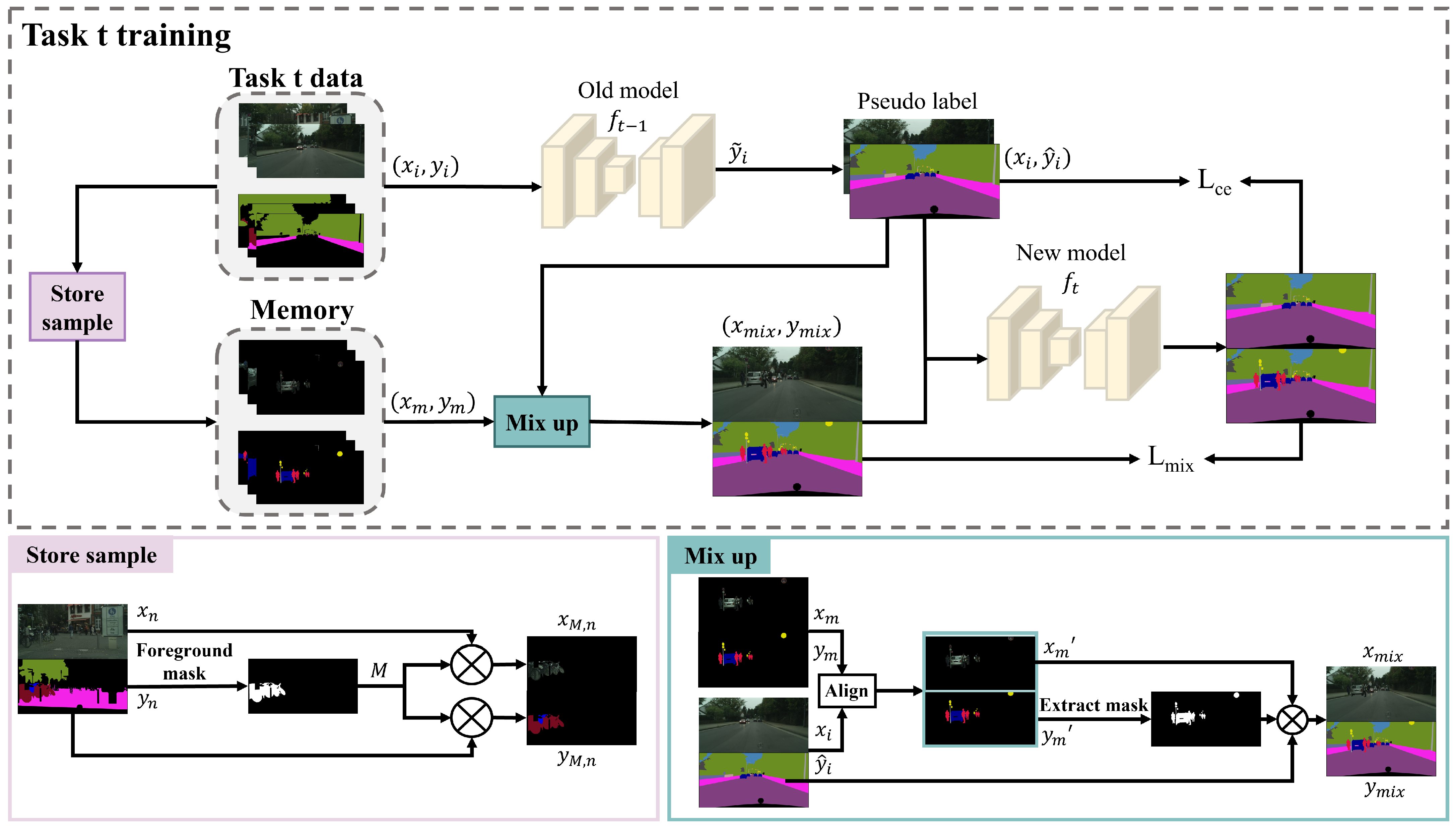
3.2. Overall Architecture

The overview of the proposed SAF is illustrated in Figure 2. During the training process for step t, $D_t$ is input into the old model obtained from step $t-1$ to generate pseudo-labels. The pseudo-labeled samples from $D_t$ are combined with replay samples from memory using SAM to obtain mixed samples. The new model is trained using both the pseudo-labeled samples and the mixed samples, yielding the losses $L_{ce}$ and $L_{mix}$, respectively. The detailed process will be described in the following. After training at step t, a randomly selected subset of samples from $D_t$ is stored in memory, with the number of samples given by the following:

$${\eta }_t={\displaystyle \frac{|D_t|}{\left|D\right|}}{\eta }_{total}$$

(1)

where $|·|$ denotes the number of elements in a set, and ${\eta }_{total}$ is the total number of samples allowed to be stored in memory.

During the initial training step (t = 1), no replay is performed, nor are pseudo-labels generated. The model is trained directly on $D_t$ using the loss $L_{ce}$.

3.3. Foreground Classes Replay

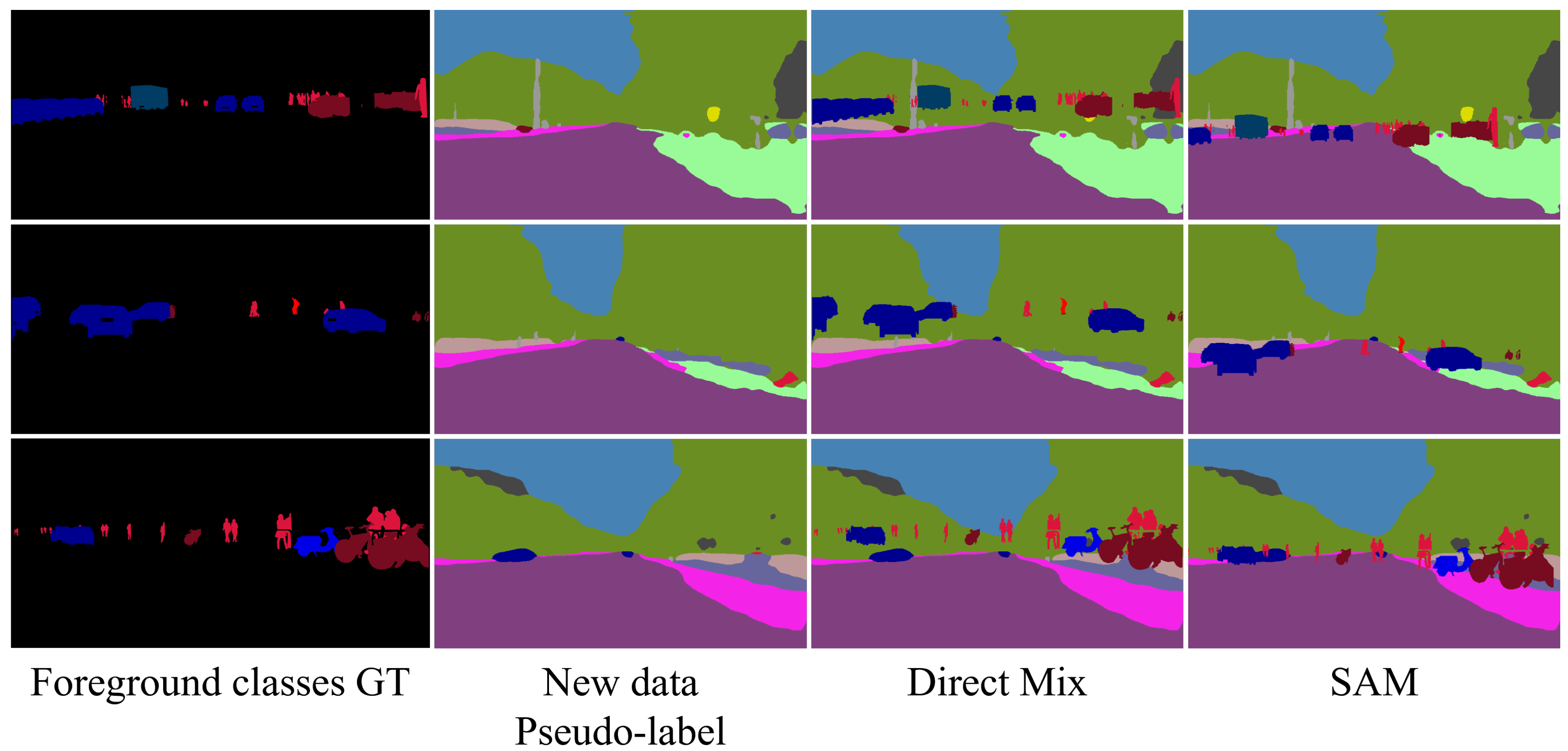
In semantic segmentation tasks, pixels from old classes repeat in subsequent samples. Particularly in autonomous driving scenarios, the pixels labeled in each incremental step are usually merely a small portion of the total pixels, and most of them are unlabeled pixels from old classes. To use information from old classes in the sample, a common method is to generate pseudo-labels using the teacher model from the previous incremental step. In the incremental step, t, of training, the pseudo-labels can be expressed as follows:

$${\widehat{y}}_i(h,w)=\left\{\begin{array}{cc}{\tilde{y}}_i(h,w),\hfill & otherwise\hfill \\ y_i(h,w),\hfill & if{y}_i(h,w)\in C_t\hfill \end{array}\right.,h\in H,w\in W$$

(2)

where H and W are the height and width of the images, $\tilde{y}$ denotes the label obtained from the step $t-1$ model, and $(x_i,{\widehat{y}}_i)$ are the samples added with pseudo-labeling for the subsequent process.

Our method focuses solely on replaying the foreground classes and storing only the relevant foreground-class information from the samples. A binary foreground mask, M, is generated to filter out the background classes in the samples $(x_n,y_n)$ to be stored, and the foreground mask M can be expressed as follows:

$$M(h,w)=\left\{\begin{array}{cc}0,\hfill & otherwise\hfill \\ 1,\hfill & if{y}_n(h,w)\in C_t\cap C_F\hfill \end{array}\right.,h\in H,w\in W$$

(3)

where $C_F$ is the foreground-class subset. Then, the foreground mask M is used to mix with $(x_n,y_n)$:

$$(x_{M,n},y_{M,n})=(M\odot x_n,M\odot y_n)$$

(4)

where ⊙ is element-wise multiplication, and $(x_{M,n},y_{M,n})$ is the stored sample. In the replay, for each new sample, $(x_i,{\widehat{y}}_i)$, we randomly select a replay sample, $(x_m,y_m)$, from the memory and use SAM to obtain a mixed sample:

$$(x_{mix,i},y_{mix,i})=Mix((x_i,{\widehat{y}}_i),(x_m,y_m))$$

(5)

where $Mix$ is SAM, described in Section 3.4. Then, we train using a mixed sample, and the loss is expressed as follows:

$$L_{mix}=-\sum _{k=1}^{H\times W}\sum _{c=1}^{C_{1:t}}{y}_{mix,i}^{(k,c)}log{P}_{mix,i}^{(k,c)}$$

(6)

where P denotes the prediction.

3.4. SAM

Given that only foreground-class information is retained, it is imperative to calculate the mixing position based on the spatial distribution of the samples during the mixing process to protect the contextual information. Therefore, we propose a simple and effective geometric matching method that aligns the ground structures across samples with a reasonable degree of accuracy. This approach ensures that foreground objects maintain a plausible spatial arrangement and reduce the adverse impact of inconsistent contextual information on the model’s performance.

The replay sample $(x_m,y_m)$ and the new sample $(x_i,{\widehat{y}}_i)$ are to be mixed samples; we extract the road contours ${\mu }_m$ and ${\mu }_i$ in $y_m$ and ${\widehat{y}}_i$ and calculate the image moments of the contours‘ convex hull. Then, the centroid coordinates of ${\mu }_m$,${\mu }_i$ can be expressed as follows:

$$(X_m,Y_m)=({\displaystyle \frac{{\mu }_m\left[m_{10}\right]}{{\mu }_m\left[m_{00}\right]}},{\displaystyle \frac{{\mu }_m\left[m_{01}\right]}{{\mu }_m\left[m_{00}\right]}})$$

(7)

$$(X_i,Y_i)=({\displaystyle \frac{{\mu }_i\left[m_{10}\right]}{{\mu }_i\left[m_{00}\right]}},{\displaystyle \frac{{\mu }_i\left[m_{01}\right]}{{\mu }_i\left[m_{00}\right]}})$$

(8)

where $m_{10}$ and $m_{01}$ represent first-order moments in the x and y directions. $m_{00}$ represents the zero-order moment. In addition, when storing the replayed samples, these centroid coordinates need to be stored. The coordinate offset $(\Delta x,\Delta y)$ can be expressed as follows:

$$(\Delta x,\Delta y)=(X_i-X_m,Y_i-Y_m)$$

(9)

We translate the image $(x_m,y_m)$ to $(x_m^{\prime },y_m^{\prime })$ based on the offset $(\Delta x,\Delta y)$. $(x_m^{\prime },y_m^{\prime })$ is the aligned image:

$$(x_m^{\prime },y_m^{\prime })=(x_m+\Delta x,y_m+\Delta y)$$

(10)

The mixing result $(x_{mix},y_{mix})$ can be expressed as follows:

$$x_{mix}=\left\{\begin{array}{cc}{x}_i(h,w),\hfill & if{y}_m^{\prime }(h,w)=0\hfill \\ x_m^{\prime }(h,w),\hfill & otherwise\hfill \end{array}\right.,h\in H,w\in W$$

(11)

$$y_{mix}=\left\{\begin{array}{cc}{\widehat{y}}_i(h,w),\hfill & if{y}_m^{\prime }(h,w)=0\hfill \\ y_m^{\prime }(h,w),\hfill & otherwise\hfill \end{array}\right.,h\in H,w\in W$$

(12)

3.5. Total Loss

In addition to the loss, $L_{mix}$, of the mixed samples, the pre-mixed sample $(x_i,y_i^{\prime })$ is used to train the model via cross-entropy loss:

$$L_{ce}=-\sum _{k=1}^{H\times W}\sum _{c=1}^{C_{1:t}}{\widehat{y}}_i^{(k,c)}log{P}_i^{(k,c)}$$

(13)

In summary, the total loss can be expressed as follows:

$$L=L_{ce}+\alpha L_{mix}$$

(14)

where $\alpha$ is the weight of the mixing loss.

4. Experiment

4.1. Experiment Setting

4.1.1. Datasets

The experiments in this paper use the Cityscapes [18] and BDD100K [19] datasets, both of which use the same 19 classes. Cityscapes is an autonomous driving dataset consisting of 2975 training images and 500 validation images captured from urban streets in European cities. BDD100K is a dataset of road scenes in the United States, covering various weather and time conditions, with 7000 training images and 1000 validation images. In the experiment, we divide the classes into background classes (road, sidewalk, building, wall, fence, vegetation, terrain, and sky) and foreground classes (other). The initial training step uses 13 classes, and the subsequent incremental steps use 6 classes. The 13 classes of the initial training step consist of eight background classes, four foreground classes (truck, bus, train, and motorcycle), and one randomly selected foreground class. Similar to the division in the paper [16], we divide the four classes (truck, bus, train, and motorcycle) into the initial thirteen classes, and the pixels of these four classes do not appear in the image of incremental steps.

4.1.2. Implementation Details

All experiments were implemented with Pytorch 1.10.0 and trained using two NVIDIA GeForce RTX 2080 Ti GPUs. The experiments used the segmentation model DeeplabV3 [33] and backbone ResNet-101 [34] pre-trained on ImageNet. During training, we cropped the image to a random region of size 768 × 768 and then used random level flip and normalization. In the initial step, we trained the model using an SGD optimizer, with a momentum of 0.9, a learning rate of $1\times {10}^{-2}$, and a weight decay of $1\times {10}^{-4}$, and we set the learning rate of the backbone network to be the optimizer learning rate divided by 10. In the incremental steps, we used a learning rate of $4\times {10}^{-3}$, and the other settings were the same as the initial step. In addition, we used the polynomial learning rate schedule [33] and set the power to 0.9. The mixed loss weight, $\alpha$, was set to 1.

4.1.3. Metrics

After the incremental steps were all over, we calculated the mean intersection over union (mIoU) for the initial step classes, incremental step classes, and all classes.

4.2. Comparison with Cityscapes

To demonstrate the effectiveness of SAF, we compared it with some classical methods. In the initial step, the model was trained using a subset containing 13 classes. In the incremental steps, the other 6 classes were trained (6, 3, and 1 per step). We compared SAF with simple replay, for which the memory size of SAF was set to 128 samples. In Cityscapes, SAF saves over 90% of memory when storing the same samples. Therefore, the memory size of simple replay was set to 16 and 128, which are similar to SAF in terms of memory occupation and number of samples stored, respectively.

The final results are shown in Table 1. Compared with other methods, SAF outperforms the other methods when setting increments to 13-6 and 13-3. At the 13-1 incremental setting, SAF is only 1.0% lower than the simple replay with the same number of stored samples of 128 while requiring approximately 10% of the memory used in simple replay for replay samples. The reduction in memory usage is due to the SAF not storing background-class information, which, while leading to a slight loss in performance, greatly enhances memory efficiency. By using both SAF and the unbiased knowledge of distillation losses in MiB, better results are achieved, outperforming the other methods in all three incremental settings. Furthermore, as the number of incremental steps increases (two steps → three steps → seven steps), the mIoU of classes learned in the initial training step exhibits varying degrees of decline. Among these, replay-based methods demonstrate a smaller decline, with SAF and simple replay (size = 128) showing only a 1.9% and 1.1% decrease, respectively. This highlights the importance of replay in mitigating catastrophic forgetting.

Table 1. Compare with classical methods on Cityscapes.

Methods	13-6 (2 Steps)			13-3 (3 Steps)				13-1 (7 Steps)
	1–13	14–19	All	1–13	14–16	17–19	All	1–13	14–19	All
offline	76.9	71.4	75.2	76.9	64.8	78.2	75.2	76.9	71.4	75.2
FT	41.3	61.7	47.7	30.8	34.2	67.7	37.1	3.9	10.7	6.1
CIL [35]	62.7	64.9	63.4	62.3	52.3	70.3	61.9	58.9	38.0	52.3
PLOP [36]	66.0	64.1	65.4	65.3	56.0	69.5	64.5	62.2	40.9	55.4
SSUL [12]	63.9	66.7	64.8	62.1	52.6	71.4	62.1	56.2	50.7	54.4
MiB [9]	64.7	65.9	65.1	64.3	55.7	70.6	63.9	62.9	41.3	56.0
Replay (size = 16)	65.3	59.3	63.4	64.9	44.0	65.3	61.7	62.2	26.1	50.8
Replay (size = 128)	68.1	58.7	65.1	67.5	52.7	63.6	64.5	67.0	46.0	60.4
Ours (size = 128)	67.6	63.0	66.1	67.1	51.3	69.2	64.9	65.7	46.3	59.6
Ours + MiB	68.9	65.4	67.8	68.5	54.3	70.9	66.6	67.3	48.7	61.4

Bold values indicate that metrics outperform other comparative incremental learning methods.

We further present qualitative results of the 13-6 incremental setting on Cityscapes in Figure 3. It can be observed that SAF performs well on certain foreground classes (e.g., bus and truck), as indicated by the white boxes. SAF correctly identifies a bus and a truck even when these objects are partially occluded by car-class objects, whereas SSUL and simple replay fail to distinguish them accurately. However, as shown in the black boxes, SAF struggles to recognize distant and smaller foreground objects (e.g., pole), the limitation was also observed in SSUL, simple replay, and even the offline training model.

Figure 3. Qualitative comparison of Cityscapes between SAF and previous methods at the incremental setting of 13-6 (two steps). The black and white box highlights the key areas for comparison.

4.3. Comparison with BDD100K

The results using BDD100k are shown in Table 2. Compared to the results using Cityscapes, most methods exhibit lower performance with BDD100k, likely due to the more complex weather and time conditions present in BDD100k. SAF has similar results to the simple replay with the same number of stored samples of 128 in the 13-6 setting, and it is 0.2% lower than PLOP. In the 13-1 setting, SAF is merely 0.3% lower than this simple replay. SAF + MiB achieve better results in all settings.

Table 2. Comparison with classical methods using BDD100k.

Methods	13-6 (2 Steps)			13-1 (7 Steps)
	1–13	14–19	All	1–13	14–19	All
Offline	59.8	51.7	57.2	59.8	51.7	57.2
FT	26.7	37.1	30.0	0.1	1.8	0.6
PLOP [36]	42.9	41.4	42.4	36.2	33.1	35.2
MiB [9]	38.7	43.0	40.1	37.9	35.9	37.3
Replay (size = 16)	39.9	38.4	39.4	37.1	19.7	36.9
Replay (size = 128)	44.2	37.8	42.2	41.9	32.4	38.9
Ours (size = 128)	43.0	40.5	42.2	41.3	32.9	38.6
Ours + MiB	43.9	42.7	43.5	41.7	33.6	39.1

Bold values indicate that metrics outperform other comparative incremental learning methods.

4.4. Replay Memory-Required Analysis

To ensure fairness in comparison, we conducted a quantitative analysis of the compression effectiveness, as shown in Table 3. We compared the average memory required for storing different numbers of replay samples under various incremental class settings for both simple replay and SAF on the Cityscapes datasets. Since simple replay stores original images, its memory requirement depends solely on the number of stored samples and is unaffected by the incremental class setting. In contrast, SAF stores only the foreground-class pixels of the current incremental step, which is influenced by the foreground classes included in each incremental step. Under conditions where all foreground classes are included in the initial step (e.g., 19-0), each replay sample must store all foreground-class pixels. It can be observed that, even in the 19-0 setting, SAF with a size of 128 requires a memory similar to simple replay with a size of 16. Under the 13-6 setting, which aligns with our experimental setup, SAF requires only 10 MB of memory, accounting for just 3.5% of the memory needed for simple replay with a size of 128.

Table 3. Comparison of memory of classical methods using Cityscapes.

Methods	Incremental Setting	Size	Memory
Replay (simple)	13-6	16	35.6 MB
		128	285 MB
	19-0	16	35.6 MB
		128	285 MB
SAF	13-6	128	10.1 MB
	19-0	128	36.2 MB

4.5. Ablation Studies

4.5.1. Effectiveness Assessment of Components

Experiments were conducted to validate the effectiveness of each component in SAF. Experiments used the Cityscapes dataset and the 13-1 incremental settings. The results are shown in Table 4. Since simple replay with a size of 16 and SAF with a size of 128 consume approximately the same amount of memory, we set the simple replay size to 16 and the foreground-class replay size to 128 in the ablation experiments. The use of foreground-class replay improves by 6.4% mIoU. Foreground-class replay enhances memory efficiency and improves the semantic richness of stored samples. Spatial adaptive alignment improves performance by 2.4%, which demonstrates that the model better learns the contextual information of old classes. Additionally, incorporating unbiased distillation loss from MiB contributes an additional 1.8% performance gain.

Table 4. Results of the ablation experiments on Cityscapes.

Components	Cityscapes 13-1 (7 Steps)
	1–13	14–19	All
Simple replay	62.2	26.1	50.8
+Foreground-class replay	64	42.6	57.2
+Spatial–adaptive alignment	65.7	46.3	59.6
+MiB [9]	67.3	48.7	61.4

Bold values indicate that metrics outperform other comparative incremental learning methods.

4.5.2. Hyperparameter

The loss function includes a hyperparameter, $\alpha$, used to balance the mixed loss. In order to test the effect of the hyperparameter on the model and determine the value that benefits the model most, we conducted experiments with different values of $\alpha$, as shown in Table 5. It can be observed that, when $\alpha =1$, the optimal mIoU for all classes is obtained. Therefore, in all other experiments, we set $\alpha =1$. Furthermore, in incremental learning, stability refers to the model’s ability to prevent forgetting old knowledge, while plasticity refers to its ability to learn new knowledge. The conflict between these two aspects constitutes the stability–plasticity dilemma in incremental learning [37]. As $\alpha$ decreases, the segmentation accuracy of the initial 13 classes gradually decreases, while the accuracy of the 6 incrementally added classes shows a slight improvement. This indicates that, as $\alpha$ decreases, our method tends to enhance the model’s plasticity in the stability–plasticity dilemma. Setting $\alpha$ to 1 effectively balances the model’s stability and plasticity.

Table 5. Results of the hyperparameter experiments on Cityscapes.

Hyperparameter	Cityscapes 13-1 (7 Steps)
$\mathbf{\alpha }$	1–13	14–19	All
10	66.1	40.9	58.1
1	65.7	46.3	59.6
0.1	64.8	46.6	59
0.01	63.3	46.8	58.1
0.001	60.9	46.7	56.5

Bold values indicate that metrics outperform other comparative incremental learning methods.

5. Conclusions

In this paper, we have proposed a replay-based CISS method SAF. To address the challenge of preserving critical semantic information in autonomous driving scenarios, the replay method of storing only foreground-class objects was proposed, which effectively improves memory efficiency. In addition, SAM mitigates the lack of contextual information and semantic confusion caused by the lack of background class information for stored samples. The experiments showed that SAF achieved competitive results. And SAF can be used as a replay module for other incremental learning tasks. Future work will focus on extending the applicability of SAF to more diverse scenarios, such as general semantic segmentation tasks, and exploring its application in domain-incremental settings to investigate the role of replay in domain-incremental learning.

References

1. Bono, F.M.; Radicioni, L.; Cinquemani, S. A novel approach for quality control of automated production lines working under highly inconsistent conditions. Eng. Appl. Artif. Intell. 2023, 122, 106149. [Google Scholar] [CrossRef]
2. Xiao, X.; Zhao, Y.; Zhang, F.; Luo, B.; Yu, L.; Chen, B.; Yang, C. BASeg: Boundary aware semantic segmentation for autonomous driving. Neural Netw. 2023, 157, 460–470. [Google Scholar] [PubMed]
3. Tavera, A.; Cermelli, F.; Masone, C.; Caputo, B. Pixel-by-pixel cross-domain alignment for few-shot semantic segmentation. In Proceedings of the IEEE/CVF Winter Conference on Applications of Computer Vision, Waikoloa, HI, USA, 3–8 January 2022; pp. 1626–1635. [Google Scholar]
4. Hong, Y.; Pan, H.; Sun, W.; Jia, Y. Deep dual-resolution networks for real-time and accurate semantic segmentation of road scenes. arXiv 2021, arXiv:2101.06085. [Google Scholar]
5. Zhao, W.; Rao, Y.; Liu, Z.; Liu, B.; Zhou, J.; Lu, J. Unleashing text-to-image diffusion models for visual perception. In Proceedings of the IEEE/CVF International Conference on Computer Vision, Paris, France, 2–6 October 2023; pp. 5729–5739. [Google Scholar]
6. Xu, M.; Zhang, Z.; Wei, F.; Hu, H.; Bai, X. Side adapter network for open-vocabulary semantic segmentation. In Proceedings of the IEEE/CVF Conference on Computer Vision and Pattern Recognition, Paris, France, 2–6 October 2023; pp. 2945–2954. [Google Scholar]
7. McCloskey, M.; Cohen, N.J. Catastrophic interference in connectionist networks: The sequential learning problem. In Psychology of Learning and Motivation; Elsevier: Amsterdam, The Netherlands, 1989; Volume 24, pp. 109–165. [Google Scholar]
8. Michieli, U.; Zanuttigh, P. Incremental learning techniques for semantic segmentation. In Proceedings of the IEEE/CVF International Conference on Computer Vision Workshops, Seoul, Republic of Korea, 27 October–2 November 2019. [Google Scholar]
9. Cermelli, F.; Mancini, M.; Bulo, S.R.; Ricci, E.; Caputo, B. Modeling the background for incremental learning in semantic segmentation. In Proceedings of the IEEE/CVF Conference on Computer Vision and Pattern Recognition, Seattle, WA, USA, 13–19 June 2020; pp. 9233–9242. [Google Scholar]
10. Michieli, U.; Zanuttigh, P. Continual semantic segmentation via repulsion-attraction of sparse and disentangled latent representations. In Proceedings of the IEEE/CVF conference on Computer Vision and Pattern Recognition, Nashville, TN, USA, 20–25 June 2021; pp. 1114–1124. [Google Scholar]
11. Baek, D.; Oh, Y.; Lee, S.; Lee, J.; Ham, B. Decomposed knowledge distillation for class-incremental semantic segmentation. Adv. Neural Inf. Process. Syst. 2022, 35, 10380–10392. [Google Scholar]
12. Cha, S.; Kim, B.; Yoo, Y.; Moon, T. Ssul: Semantic segmentation with unknown label for exemplar-based class-incremental learning. Adv. Neural Inf. Process. Syst. 2021, 34, 10919–10930. [Google Scholar]
13. Maracani, A.; Michieli, U.; Toldo, M.; Zanuttigh, P. Recall: Replay-based continual learning in semantic segmentation. In Proceedings of the IEEE/CVF International Conference on Computer Vision, Montreal, BC, Canada, 11–17 October 2021; pp. 7026–7035. [Google Scholar]
14. Chen, J.; Cong, R.; Luo, Y.; Ip, H.; Kwong, S. Saving 100× storage: Prototype replay for reconstructing training sample distribution in class-incremental semantic segmentation. Adv. Neural Inf. Process. Syst. 2024, 36, 35988–35999. [Google Scholar]
15. Van de Ven, G.M.; Siegelmann, H.T.; Tolias, A.S. Brain-inspired replay for continual learning with artificial neural networks. Nat. Commun. 2020, 11, 4069. [Google Scholar] [PubMed]
16. Kalb, T.; Roschani, M.; Ruf, M.; Beyerer, J. Continual learning for class-and domain-incremental semantic segmentation. In Proceedings of the 2021 IEEE Intelligent Vehicles Symposium (IV), Nagoya, Japan, 11–17 July 2021; pp. 1345–1351. [Google Scholar]
17. Kalb, T.; Mauthe, B.; Beyerer, J. Improving replay-based continual semantic segmentation with smart data selection. In Proceedings of the 2022 IEEE 25th International Conference on Intelligent Transportation Systems (ITSC), Macau, China, 8–12 October 2022; pp. 1114–1121. [Google Scholar]
18. Cordts, M.; Omran, M.; Ramos, S.; Rehfeld, T.; Enzweiler, M.; Benenson, R.; Franke, U.; Roth, S.; Schiele, B. The cityscapes dataset for semantic urban scene understanding. In Proceedings of the IEEE Conference on Computer Vision and Pattern Recognition, Las Vegas, NV, USA, 27–30 June 2016; pp. 3213–3223. [Google Scholar]
19. Yu, F.; Chen, H.; Wang, X.; Xian, W.; Chen, Y.; Liu, F.; Madhavan, V.; Darrell, T. Bdd100k: A diverse driving dataset for heterogeneous multitask learning. In Proceedings of the IEEE/CVF Conference on Computer Vision and Pattern Recognition, Seattle, WA, USA, 13–19 June 2020; pp. 2636–2645. [Google Scholar]
20. Wickramasinghe, B.; Saha, G.; Roy, K. Continual learning: A review of techniques, challenges, and future directions. IEEE Trans. Artif. Intell. 2023, 5, 2526–2546. [Google Scholar]
21. Aljundi, R.; Babiloni, F.; Elhoseiny, M.; Rohrbach, M.; Tuytelaars, T. Memory aware synapses: Learning what (not) to forget. In Proceedings of the European Conference on Computer Vision (ECCV), Munich, Germany, 8–14 September 2018; pp. 139–154. [Google Scholar]
22. Li, Z.; Hoiem, D. Learning without forgetting. IEEE Trans. Pattern Anal. Mach. Intell. 2017, 40, 2935–2947. [Google Scholar] [PubMed]
23. Castro, F.M.; Marín-Jiménez, M.J.; Guil, N.; Schmid, C.; Alahari, K. End-to-end incremental learning. In Proceedings of the European Conference on Computer Vision (ECCV), Munich, Germany, 8–14 September 2018; pp. 233–248. [Google Scholar]
24. Douillard, A.; Cord, M.; Ollion, C.; Robert, T.; Valle, E. Podnet: Pooled outputs distillation for small-tasks incremental learning. In Proceedings of the Computer Vision—ECCV 2020: 16th European Conference, Glasgow, UK, 23–28 August 2020; Proceedings, Part XX 16. Springer: Berlin/Heidelberg, Germany, 2020; pp. 86–102. [Google Scholar]
25. Li, X.; Zhou, Y.; Wu, T.; Socher, R.; Xiong, C. Learn to grow: A continual structure learning framework for overcoming catastrophic forgetting. In Proceedings of the International Conference on Machine Learning, PMLR, Long Beach, CA, USA, 9–15 June 2019; pp. 3925–3934. [Google Scholar]
26. Singh, P.; Mazumder, P.; Rai, P.; Namboodiri, V.P. Rectification-based knowledge retention for continual learning. In Proceedings of the IEEE/CVF Conference on Computer Vision and Pattern Recognition, Nashville, TN, USA, 20–25 June 2021; pp. 15282–15291. [Google Scholar]
27. Yan, S.; Xie, J.; He, X. Der: Dynamically expandable representation for class incremental learning. In Proceedings of the IEEE/CVF Conference on Computer Vision and Pattern Recognition, Nashville, TN, USA, 20–25 June 2021; pp. 3014–3023. [Google Scholar]
28. Rebuffi, S.A.; Kolesnikov, A.; Sperl, G.; Lampert, C.H. icarl: Incremental classifier and representation learning. In Proceedings of the IEEE Conference on Computer Vision and Pattern Recognition, Honolulu, HI, USA, 21–25 July 2017; pp. 2001–2010. [Google Scholar]
29. Wu, C.; Herranz, L.; Liu, X.; Van De Weijer, J.; Raducanu, B. Memory replay gans: Learning to generate new categories without forgetting. Adv. Neural Inf. Process. Syst. 2018, 31, 5966–5976. [Google Scholar]
30. Hayes, T.L.; Kafle, K.; Shrestha, R.; Acharya, M.; Kanan, C. Remind your neural network to prevent catastrophic forgetting. In Proceedings of the European Conference on Computer Vision, Glasgow, UK, 23–28 August 2020; Springer: Berlin/Heidelberg, Germany, 2020; pp. 466–483. [Google Scholar]
31. Michieli, U.; Zanuttigh, P. Knowledge distillation for incremental learning in semantic segmentation. Comput. Vis. Image Underst. 2021, 205, 103167. [Google Scholar]
32. Goodfellow, I.; Pouget-Abadie, J.; Mirza, M.; Xu, B.; Warde-Farley, D.; Ozair, S.; Courville, A.; Bengio, Y. Generative adversarial nets. Adv. Neural Inf. Process. Syst. 2014, 27, 2672–2680. [Google Scholar]
33. Chen, L.C. Rethinking atrous convolution for semantic image segmentation. arXiv 2017, arXiv:1706.05587. [Google Scholar]
34. He, K.; Zhang, X.; Ren, S.; Sun, J. Deep residual learning for image recognition. In Proceedings of the IEEE Conference on Computer Vision and Pattern Recognition, Las Vegas, NV, USA, 27–30 June 2016; pp. 770–778. [Google Scholar]
35. Klingner, M.; Bär, A.; Donn, P.; Fingscheidt, T. Class-incremental learning for semantic segmentation re-using neither old data nor old labels. In Proceedings of the 2020 IEEE 23rd International Conference on Intelligent Transportation Systems (ITSC), Rhodes, Greece, 20–23 September 2020; pp. 1–8. [Google Scholar]
36. Douillard, A.; Chen, Y.; Dapogny, A.; Cord, M. Plop: Learning without forgetting for continual semantic segmentation. In Proceedings of the IEEE/CVF Conference on Computer Vision and Pattern Recognition, Nashville, TN, USA, 20–25 June 2021; pp. 4040–4050. [Google Scholar]
37. Araujo, V.; Hurtado, J.; Soto, A.; Moens, M.F. Entropy-based stability-plasticity for lifelong learning. In Proceedings of the IEEE/CVF Conference on Computer Vision and Pattern Recognition, New Orleans, LA, USA, 18–24 June 2022; pp. 3721–3728. [Google Scholar]