Insights into Mosquito Behavior: Employing Visual Technology to Analyze Flight Trajectories and Patterns

Abstract

Mosquitoes, as vectors of numerous serious infectious diseases, require rigorous behavior monitoring for effective disease prevention and control. Simultaneously, precise surveillance of flying insect behavior is also crucial in agricultural pest management. This study proposes a three-dimensional trajectory reconstruction method for mosquito behavior analysis based on video data. By employing multiple synchronized cameras to capture mosquito flight images, using background subtraction to extract moving targets, applying Kalman filtering to predict target states, and integrating the Hungarian algorithm for multi-target data association, the system can automatically reconstruct three-dimensional mosquito flight trajectories. Experimental results demonstrate that this approach achieves high-precision flight path reconstruction, with a detection accuracy exceeding 95%, an F1-score of 0.93, and fast processing speeds that enables real-time tracking. The mean error of three-dimensional trajectory reconstruction is only 10 ± 4 mm, offering significant improvements in detection accuracy, tracking robustness, and real-time performance over traditional two-dimensional methods. These findings provide technological support for optimizing vector control strategies and enhancing precision pest control and can be further extended to ecological monitoring and agricultural pest management, thus bearing substantial significance for both public health and agriculture.

1. Introduction

The prevention and control of mosquito-borne infectious diseases has always been a major challenge in the field of global public health. As an important vector for pathogens, such as dengue fever [1,2], malaria [3,4], and lymphatic filariasis [5,6], there is a significant correlation between the flight trajectory of mosquitoes, their host selection behavior, and the efficiency of disease transmission. Especially in recent years, the acceleration of global climate change and urbanization process has led to a new transmission trend of mosquito-borne diseases, and there is an urgent need to establish prevention and control strategies based on fine behavior monitoring. In addition, mosquitoes not only play the role of pollination in the ecosystem but also play an important role in population regulation. The dynamic analysis of their three-dimensional migration paths is of great significance for maintaining biodiversity. Research in the agricultural field also shows that the harm caused by specific mosquito species to crops has a spatial correlation with their activity trajectories. Therefore, traditional two-dimensional observation methods can no longer meet the research needs of multiple disciplines.

There are significant technical bottlenecks in traditional methods for mosquito behavior research. Currently, the mainstream research methods mainly include two categories. The first is the manual visual observation method. Researchers need to conduct field investigations in the wild or conduct static observations in a controlled experimental device. However, mosquito individuals are generally at the millimeter scale (with a body length usually ranging from 2 to 10 mm). The human eye is prone to problems such as visual fatigue and instant omissions when continuously capturing micro-movements, resulting in the observation results being affected by subjective cognitive biases. The second is the video recording based on fixed camera devices combined with the manual trajectory analysis method. Although it can reduce the interference of observers to a certain extent, due to the need to maintain a safe shooting distance to avoid changing the natural behavior pattern of mosquitoes, the imaging resolution is severely limited. In the conventional field of view, mosquitoes usually only occupy a few pixels, and the motion blur effect is more likely to occur during high-speed movement. It is worth noting that the drone dynamic tracking technology developed by the Vo-Doan research team [7] provides a new idea for insect behavior recording. This solution achieves non-contact observation through a mobile shooting platform. Nevertheless, the dynamic focusing delay and trajectory prediction error of miniature targets remain technical difficulties.

In recent years, with the rapid development of computer vision and deep learning technologies, significant progress has been made in the research on the detection and tracking of small targets such as mosquitoes. Firstly, visual-based mosquito behavior monitoring technology has been widely applied. Javed et al. [8] used the Mask R-CNN algorithm to achieve high-precision detection and tracking of flying and stationary mosquitoes, significantly improving the efficiency of behavior feature extraction. Wang J T et al. [9] combined deep learning and computer vision technologies to develop an efficient insect monitoring system, providing a new tool for population dynamics analysis. In addition, Spitzen et al. [10,11] developed a special wind tunnel and Track3D software (developed by Noldus Information Technology as an add-on to EthoVision v3.1 [10])to optimize the automatic tracking and analysis of the three-dimensional trajectories of mosquitoes, especially showing advantages in the research on nighttime navigation and host positioning.

Although the target detection and tracking algorithms based on deep learning perform excellently in the applications of macroscopic targets such as pedestrians and vehicles, when directly transferred to small targets such as mosquitoes, their performance shows an obvious decline. The sub-pixel-level imaging characteristics of mosquitoes lead to a decrease in the feature extraction efficiency of traditional convolutional neural networks, and the false positive rate and false negative rate increase significantly under the interference of complex backgrounds. More importantly, most of the existing methods are limited to the analysis of two-dimensional planar trajectories, while the real movement trajectories of mosquitoes have typical three-dimensional spatial characteristics, which requires the development of a new stereo vision analysis framework.

In response to these challenges, this paper introduces a mosquito behavior analysis framework grounded in background subtraction, multi-target tracking, and stereo vision, capable of precisely capturing three-dimensional flight trajectories. This method refines the detection of small targets, bolsters tracking stability across multiple viewpoints, and leverages a binocular vision geometric model for trajectory reconstruction. The key contributions are as follows:

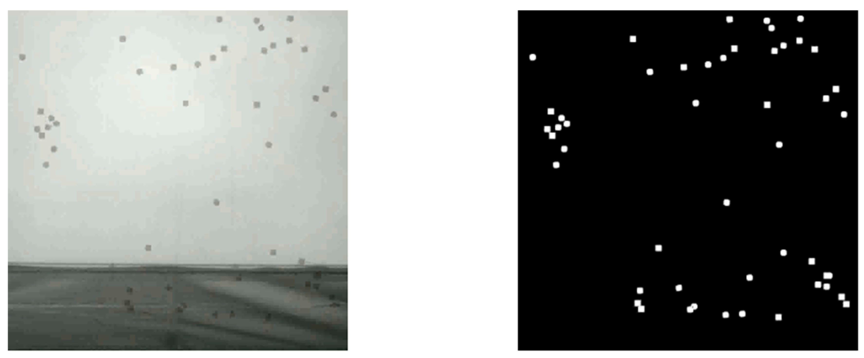
• A motion target detection approach based on background subtraction: By constructing an updated adaptive background model, it accurately isolates foreground objects from complex backdrops, thereby enhancing detection robustness and precision.
• A multi-target tracking algorithm integrating the Kalman filter prediction and the Hungarian algorithm-based data association: For each camera view, targets are tracked using a fusion of the Kalman filter and the Hungarian algorithm, ensuring continuous target identities across consecutive frames via state prediction and optimal matching, thus providing reliable and stable multi-object tracking.
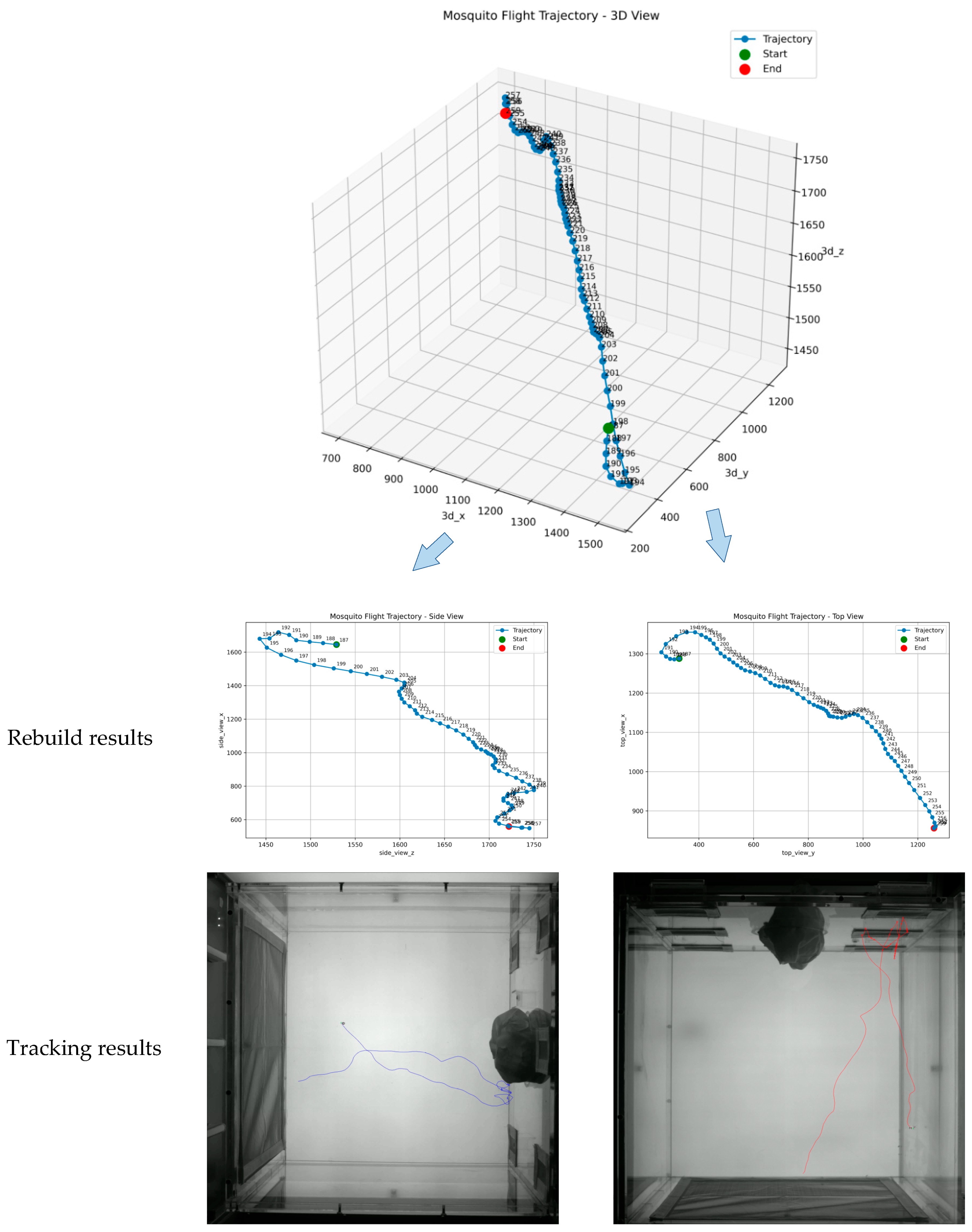
• A stereoscopic 3D trajectory reconstruction scheme tailored to small objects such as mosquitoes: By merging the two-dimensional detections from different viewpoints to calculate three-dimensional coordinates, this method reconstructs the authentic flight paths of the targets, overcoming the constraints of traditional 2D analysis and offering a more intuitive perspective for mosquito behavior research.

2. Related Works

2.1. Background Subtraction Algorithm

When performing multi-target tracking of mosquitoes in a video sequence, the detection of moving targets is a crucial step. Due to the extremely small volume of mosquito targets and the lack of obvious textures and features, traditional feature-based detection methods are difficult to apply effectively. Therefore, the background subtraction algorithm has become an effective choice for detecting moving targets. This algorithm extracts the position of the moving target by subtracting the current frame from the background model and thresholding the result. It is especially suitable for scenarios where the camera is stationary and can accurately detect the foreground targets.

The core of the background subtraction algorithm lies in the construction and update of the background model. By modeling each pixel point using statistical and probabilistic methods, the background subtraction algorithm can better meet the detection requirements of tiny targets. In recent years, a variety of algorithms based on statistical models and machine learning techniques have been proposed and applied: The Gaussian Mixture Model (MOG2) proposed by Zivkovic et al. [12] demonstrates excellent performance in dealing with dynamic environments. It models each pixel point using a mixture model of multiple Gaussian distributions, adaptively adjusting parameters such as mean, variance, and weight to accurately distinguish between foreground and background. However, this algorithm has a high computational complexity. In scenarios with large-scale data processing or extremely high real-time requirements, it faces performance bottlenecks. Moreover, for small and feature-less objects, its detection accuracy is poor.

The Visual Background Extractor (ViBe) algorithm [13] employs a neighborhood pixel sampling strategy. It randomly selects pixels within the neighborhood of each pixel point and stores them in the background table. During the detection phase, the current pixel is compared with the samples in the background table. If there are enough matches, it is judged as the background; otherwise, it is considered the foreground. This method utilizes local neighborhood information and does not require complex global background model updates, showing significant advantages in detecting fast-moving objects. However, it is sensitive to background noise and illumination changes. When the background has complex textures or unstable illumination conditions, false positives or false negatives are likely to occur. In addition, when the color of the target is similar to that of the background, the detection accuracy will also be affected.

Compared with the Gaussian Mixture Model (MOG2) and the Visual Background Extractor (ViBe) algorithm, the K-Nearest Neighbor (KNN)-based algorithm [14] has unique advantages in foreground detection. KNN determines the foreground by analyzing the relationship between pixel points and their neighborhoods. It does not rely on the Gaussian assumption of pixel grayscale values or color distributions, thus showing better adaptability to complex scenes.

Meanwhile, when utilizing neighborhood information, KNN can more comprehensively analyze local structural features and accurately capture the contour and shape information of target objects. This makes it especially suitable for cases where the target objects have complex textures or shapes. In addition, in complex detection tasks, such as multi-target detection, and when the colors of the targets are similar to the background, KNN can balance the detection accuracy and complexity by choosing appropriate K values and distance metrics, demonstrating stronger robustness and flexibility.

However, it is worth noting that there are still obvious gaps in the research of these algorithms in the field of detecting tiny and fast targets such as mosquitoes. Most of the existing literature focuses on the detection of targets of conventional sizes (such as pedestrians and vehicles). For mosquito targets with a body length of only 2–5 mm and a movement speed of up to 1.5 m/s, problems such as the lack of features caused by their tiny volume and the motion blur caused by high-speed movement have not been fully studied. Especially, when the target enters an area with a color similar to the background, traditional algorithms are prone to detection failures, which provides a necessary basis for the algorithm performance comparison study carried out in this paper.

2.2. Multiple Object Tracking

In the task of multiple object tracking (MOT), it is first necessary to identify the targets by drawing target bounding boxes and obtaining the centroid coordinates of the targets, thus laying the foundation for subsequent target tracking. After obtaining the centroid coordinates of the targets, the Kalman filter is often used for target motion prediction and correction. Since the moving target detector cannot distinguish between different targets and can only identify moving targets, the Hungarian algorithm, as a classic matching algorithm, can effectively associate the targets between adjacent frames, thus achieving accurate multi-target tracking.

The Kalman filter method is widely regarded as a classic solution in the field of MOT. Research by Welch and Bishop [15] not only elaborates on the theoretical basis of the Kalman filter but also provides solid theoretical support for its application in target tracking. Subsequently, Chen X et al. [16] further demonstrated the effectiveness of the unscented Kalman filter technology in tracking multiple moving targets. Straw et al. [17] designed a real-time multi-target tracking system based on the extended Kalman filter, which is capable of synchronously capturing the position and posture of flying animals with a delay as low as 40 milliseconds, significantly enhancing the timeliness of dynamic behavior analysis. With the rapid development of deep learning technology, the MOT methods based on deep learning have gradually become a research hotspot, especially achieving remarkable progress in the two subtasks of target prediction and data association. Target prediction focuses on using historical data and motion models to estimate the future states (such as position, velocity, and posture) of the targets, and these predictions are crucial for subsequent data association. Data association aims to accurately match the observed data with the targets to ensure accurate tracking in consecutive frames.

In the field of MOT, the SORT [18] and DeepSORT [19] algorithms perform particularly well. The DeepSORT algorithm innovatively combines deep learning with traditional target-tracking methods. Specifically, this algorithm uses a convolutional neural network (CNN) to extract the deep features of the targets, performs state estimation and prediction through the Kalman filter, and applies the Hungarian algorithm [20] for data association. In contrast, the SORT algorithm adopts a more traditional target feature representation method, such as the position information of the targets. Although it is not as accurate and robust as DeepSORT, the SORT algorithm performs more excellently in terms of real-time performance and is especially suitable for small target-tracking tasks with high real-time requirements.

2.3. Three-Dimensional Trajectory Reconstruction

Three-dimensional trajectory reconstruction is the key to analyzing mosquito behavior. Khan et al. [21] conducted an accurate behavioral analysis of mosquito activities through a multi-camera system and three-dimensional virtual environment simulation. Cheng et al. [22,23] proposed a three-dimensional group flight tracking method based on a line reconstruction algorithm, which provides a new perspective for the study of the dense movement of insects such as fruit flies.

Although existing research has promoted the development of mosquito behavior monitoring technology, there are still challenges such as difficulties in detecting small targets, limitations in tracking high-speed movements, and insufficient accuracy of three-dimensional reconstruction. Mosquitoes often appear as sub-pixel points with a low signal-to-noise ratio in videos, and mainstream algorithms are prone to noise interference. Most of the existing multi-target tracking algorithms are designed for low-speed targets and are difficult to match the characteristics of mosquitoes, such as large cross-frame displacements and non-linear movement trajectories [24]. Three-dimensional methods such as binocular vision are likely to cause trajectory distortion due to detection errors, and the cross-view target association algorithms lack robustness.

In response to the above issues, this study proposes a three-dimensional trajectory reconstruction framework for mosquitoes that integrates the improved background subtraction method, the Kalman filter, and the Hungarian algorithm. It optimizes the noise suppression ability for small target detection, and in combination with the spatiotemporal correlation strategy across cameras, it achieves robust tracking under high-speed movement. Meanwhile, by using the orthogonal binocular vision geometric model, the two-dimensional trajectory is mapped into the three-dimensional space, overcoming the limitations of traditional two-dimensional analysis. This method provides high-precision data for research on mosquito flight patterns, host selection, and migration behaviors, and lays the technical foundation for the optimization of disease transmission risk assessment and agricultural pest control strategies.

3. Methodology

3.1. Background Subtraction Based on K-Nearest Neighbor

In the field of moving target segmentation, the background subtraction algorithm based on K-Nearest Neighbor (KNN) ingeniously transforms this problem into a binary classification problem of foreground and background. Relying on the powerful machine learning method of KNN, this algorithm conducts an in-depth analysis of a single pixel point and uses the non-parametric kernel probability density estimation method to construct the background model. The basic flow is shown in Figure 1.

Suppose that the pixel value at time $t$ is ${\overrightarrow{x}}^{(t)}$, and the samples within the past time period $T$ are ${\chi }_T=\{x_t,x_{t-1}\dots x_{t-T}\}$. In order to clearly distinguish whether a sample belongs to the foreground or the background, a label $b^m$ is introduced. When $b^m=1$, the historical pixel is labeled as the background; otherwise, it is labeled as the foreground. Based on this, the background model is accurately described by the following formula:

$${\widehat{p}}_{non-parametric}(\overrightarrow{x}|X_T,BG)={\displaystyle \frac{1}{TV}}{\displaystyle \sum _{m=t-T}^t{b}^{(m)}}K({\displaystyle \frac{\left|\right|{\overrightarrow{x}}^{(m)}-\overrightarrow{x}\left|\right|}{D}})$$

(1)

Among them, $K(u)$ is a uniform kernel density function. When $\mathrm{u}\le 0.5$, $K(u)=1$, and in other cases, $K(u)=0$. $D$ is the bandwidth, and $V$ is a region with $D$ as the diameter. After constructing the background model at the $t-1$ moment, it is used to judge the new pixel point at the $t$ moment. By calculating the correlation value between the new pixel point and the background model, the larger the value ${\widehat{p}}_{non-parametric}(\overrightarrow{x}|X_T,BG)$, the greater the probability that the pixel point belongs to the background model. When the value is greater than the threshold, it is determined to be the background.

In practical applications, first, the Euclidean distance between the current pixel point and the historical pixel is calculated. If this distance is greater than half of $D$, then one should check whether the information of this historical pixel is the background. If so, the counter $k$ should be increased by 1. When $k$ is greater than the threshold $k_{thr}$, the current pixel point is recognized as the background; otherwise, it is recognized as the foreground. Finally, a binary image for foreground–background segmentation is obtained. Let $F^{(t)}(x,y)$ represent the pixel value.

$$F^{(t)}(x,y)=\left\{\begin{array}{l}255 if\hspace{1em}k>k_{thr}\hspace{1em}\hfill \\ 0\hspace{1em}if\hspace{1em}k⩽k_{thr}\hspace{1em}\hfill \end{array}\right.$$

(2)

3.2. Target Tracking

This paper adopts a method combining the Kalman filter and the Hungarian algorithm to achieve precise tracking of the movement trajectories of mosquitoes. Considering that mosquitoes fly at high speeds and have strong maneuverability, it is difficult to accurately describe their motion states using the traditional constant-velocity model [25]. Although the variable-acceleration motion model can more precisely depict the movement of mosquitoes, it will significantly increase the system complexity and computational cost. In contrast, the constant-acceleration model [26] has been widely validated in practical applications. It can not only effectively simplify the mosquito motion model but also roughly capture the range of their motion trends and acceleration changes. Therefore, this paper selects the linear Kalman filter to estimate the current state of mosquito targets in real-time.

The Kalman filter can accurately obtain the position, velocity, and acceleration information of the target by fusing the measured values and the predicted values of the model. In the case of target loss or occlusion, it can also accurately predict the target state at the current moment based on the previous state information. When tracking the trajectories of mosquitoes in a video sequence, due to the tiny size of mosquitoes, they are simplified as mass points, and the focus is on the position changes. Their motion is decomposed into constant-acceleration motions in the x- and y-axis directions. The state-transition matrix is used to describe the state changes of mosquitoes between adjacent frames and follows the laws of the constant-acceleration motion model.

Let us assume that the current moment is $t$ and the previous moment is $t-1$, and the state transition needs to satisfy the laws of constant-acceleration motion:

$$\left[\begin{array}{c}y(t)\\ v_x(t)\end{array}\right]=\left[\begin{array}{cc}1& \mathrm{\Delta }t\\ 0& 1\end{array}\right]\left[\begin{array}{c}y(t-1)\\ v_x(t-1)\end{array}\right]+\left[\begin{array}{c}{\displaystyle \frac{{(\mathrm{\Delta }t)}^2}{2}}\\ \mathrm{\Delta }t\end{array}\right]a_x(t-1)$$

(3)

$$\left[\begin{array}{c}y(t)\\ v_y(t)\end{array}\right]=\left[\begin{array}{cc}1& \mathrm{\Delta }t\\ 0& 1\end{array}\right]\left[\begin{array}{c}y(t-1)\\ v_y(t-1)\end{array}\right]+\left[\begin{array}{c}{\displaystyle \frac{{(\mathrm{\Delta }t)}^2}{2}}\\ \mathrm{\Delta }t\end{array}\right]a_y(t-1)$$

(4)

Here, $\mathrm{\Delta }t$ represents the time interval, which indicates the time difference between two time points. $x(t)$ represents the position of the $x$-axis at time $t$, $v_x(t)$ represents the velocity in the $x$-axis direction at time $t$, and $a_x(t)$ represents the acceleration in the $x$-axis direction at time $t$. The same can be deduced by analogy for the $y$-axis direction.

However, in actual situations, the acceleration is unknown. Therefore, the acceleration is regarded as the unknown noise in the state-transition process. Then, the state variable is set as a four-dimensional variable containing $x,v_x,y,v_y$. At the same time, according to the laws of constant-acceleration motion, the state-transition matrix can be obtained. For target tracking in a two-dimensional plane, the observed values are only pixel coordinates $(x,y)$. Therefore, the state variable $z_t$, the state-transition matrix $A$, and the observation matrix $C$ are as follows:

$$z_t=\left[\begin{array}{cccc}x(t)& y(t)& v_x(t)& v_y(t)\end{array}\right]$$

(5)

$$A=\left[\begin{array}{cccc}1& 0& \mathrm{\Delta }t& 0\\ 0& 1& 0& \mathrm{\Delta }t\\ 0& 0& 1& 0\\ 0& 0& 0& 1\end{array}\right]$$

(6)

$$C=\left[\begin{array}{cccc}1& 0& 0& 0\\ 0& 1& 0& 0\end{array}\right]$$

(7)

According to the process model, the relationship between the covariances of state variables can be obtained. Given that the state transition noise covariance matrix is $Q$, and assuming that the covariance matrix of the state variable is $G$, then we have:

$$G_{t+1}=A{G}_t{A}^T+Q_t$$

(8)

According to the constant-acceleration motion model, we can assume that the acceleration is noise, and the variance of the acceleration is ${\sigma }_a^2$. According to the displacement formula of constant-acceleration motion, the influence of acceleration on position and velocity can be expressed as $\mathrm{\Delta }{t}^2/2$. Therefore, the process noise covariance matrix can be obtained as follows:

$$Q=\left[\begin{array}{cccc}{\displaystyle \frac{{(\mathrm{\Delta }t)}^4}{4}}& 0& {\displaystyle \frac{{(\mathrm{\Delta }t)}^3}{2}}& 0\\ 0& {\displaystyle \frac{{(\mathrm{\Delta }t)}^4}{4}}& 0& {\displaystyle \frac{{(\mathrm{\Delta }t)}^3}{2}}\\ {\displaystyle \frac{{(\mathrm{\Delta }t)}^3}{2}}& 0& {(\mathrm{\Delta }t)}^2& 0\\ 0& {\displaystyle \frac{{(\mathrm{\Delta }t)}^3}{2}}& 0& {(\mathrm{\Delta }t)}^2\end{array}\right]$$

(9)

After predicting and estimating the target state through the Kalman filter, it is also necessary to use the Hungarian algorithm for target matching to establish the correspondence between targets in different frames, to achieve continuous tracking of multiple targets.

The Hungarian algorithm is an optimization algorithm designed to solve the assignment problem. Its core objective is to find the assignment scheme with the minimum cost under the one-to-one assignment condition. Based on graph theory, this algorithm transforms the assignment problem into a maximum-weight matching problem. It iteratively increases the feasible matchings until the optimal matching scheme is obtained. In multi-target tracking, the Hungarian algorithm matches the current detection results with the previous tracking targets and combines the estimation and prediction of the detection results using the Kalman filter to successfully construct the target trajectories (Figure 2). The workflow involves four key stages: image acquisition, moving object detection, data association, and trajectory management. The green-filled area in Figure 2 highlights the optimal matching results derived from solving the bipartite graph’s minimum weight matching problem using the Euclidean distance metrics and the Kalman-predicted velocity ellipses.

Among them, the data association and trajectory management parts form the cost matrix, and the green-filled area represents the matching results. Whenever a moving target is detected in a new frame, it is necessary to match it with the existing trajectories. Creating a cost matrix is the first step in the matching process. The rows of the matrix represent the current detection results, and the columns represent the previous tracking targets (i.e., the existing trajectories). The elements of the matrix are the matching costs, which can be measured by the Euclidean distance, the Mahalanobis distance, the intersection-over-union ratio, appearance similarity, etc. Taking targets such as mosquitoes, which are extremely small and move rapidly, as an example, due to the large difference in position between consecutive frames, the intersection-over-union ratio is often 0. Moreover, mosquitoes lack distinct appearance features, making it difficult to match based on appearance features. Given that the aim of this study is to plot the target trajectories and only the target positions are of concern, using the Euclidean distance as the matching cost is the most appropriate. By calculating the Euclidean distance, the matching costs of each target can be obtained, and thus a cost matrix can be constructed. Performing the best matching on it can complete the matching between the current detection results and the tracking targets. An example of the cost matrix is shown in Figure 3.

However, directly calculating the Euclidean distance between the tracking target points and the detection result points has problems such as insensitivity to the target position and deformation, and failure to consider the target displacement, which is likely to lead to inaccurate matching results. For small targets like mosquitoes with asymmetric and irregular shapes, using an ellipse to describe their shapes and adapt to shape changes is more effective. The Kalman filter can predict the current position and velocity information based on the target’s previous and past states. Accordingly, an ellipse is constructed at the predicted position to represent the possible shape and position of the target at the current moment. The center point of the ellipse is the predicted position, and the major and minor axes reflect the change range of the target at the current moment. The predicted ellipse of a single target is shown in Figure 4.

The yellow dot represents the detection result point at the current moment, and the blue dot represents the prediction point of the Kalman filter at the current moment. $\overrightarrow{v}$ is the velocity predicted by the Kalman filter, and $\overrightarrow{v_x},\overrightarrow{v_y}$ are the velocity components in the two axial directions. After calculating the predicted elliptical region, its angle needs to be adjusted. Let the displacement vector be $\overrightarrow{v}\mathrm{\Delta }t$. If the modulus of the displacement vector is too small, the adjustment has little significance. Therefore, the adjustment is carried out only when the modulus exceeds a certain threshold, and finally, the predicted elliptical region of the target is obtained. To consider the influence of displacement on target matching, the Euclidean distance is weighted by judging whether the detection result target point is inside the ellipse.

Suppose the current target point is $(x_0,y_0)$, the center of the predicted elliptical region is $(x_p,y_p)$, the rotation angle of the ellipse is $\theta$, and the lengths of the major and minor axes are $a$ and $b$, respectively. The following formula can be used for judgment:

$$R={\left({\displaystyle \frac{(x-x_p)\cos (\theta )+(y-y_p)\sin (\theta )}{a}}\right)}^2+{\left({\displaystyle \frac{(x-x_p)\sin (\theta )-(y-y_p)\cos (\theta )}{b}}\right)}^2$$

(10)

In the above formula, $R$ is the distance weight value. The larger the value of $R$, the more the target deviates from the predicted region; the smaller the value of $R$, the closer the target is to the predicted region.

If $R>1$, it indicates that the current detection result target point is outside the predicted elliptical region, and the target deviates from the predicted position. At this time, the Euclidean distance between the detection result point and the tracking target point is directly adopted.

If $R<1$, it indicates that the current detection result target point is inside the predicted elliptical region, and the prediction is relatively accurate. Then, the Euclidean distance is assigned a weight $R$. This weight adjustment strategy can make better use of the prediction information in multi-target tracking and effectively improve the robustness and accuracy of multi-target tracking.

Suppose the number of currently detected targets is $M$, and the number of tracking targets in the previous moment is $N$. According to the above-mentioned weight-setting method, by calculating the Euclidean distance between the detected targets and the tracking targets, an $M\times N$ cost matrix can be constructed. Performing the Hungarian algorithm on this cost matrix yields the matching results for each detected target and tracking target. However, during the tracking process, situations such as the target leaving the screen, loss of detection, or a new target entering the screen may occur. Therefore, a trajectory management method is needed to screen the trajectories. The specific operation is to add or delete the corresponding columns in the cost matrix.

3.3. Trajectory Screening and Three-Dimensional Reconstruction

Tracking small, fast-moving targets such as mosquitoes often leads to trajectory data with discontinuities and instability, primarily due to image noise, rapid movement, and occasional occlusions. To ensure the reliability of 3D reconstruction, it is necessary to perform rigorous trajectory screening prior to spatial modeling.

To begin with, we applied a minimum trajectory length threshold of 20 frames to eliminate short, unreliable tracks likely caused by noise or false detections. Additionally, a continuity ratio threshold of 80% was used to ensure that valid data points span a sufficient portion of the trajectory, effectively removing fragmented or intermittent sequences. Trajectories were also evaluated for abnormal velocity fluctuations, estimated using Kalman filtering, and those exceeding acceptable thresholds were discarded. These criteria collectively enhance the quality and consistency of the data used for reconstruction.

To further improve trajectory smoothness, a least-squares fitting method was applied to the filtered data using quadratic polynomial equations based on a constant-acceleration motion model. As mosquito flight can be reasonably approximated by uniform acceleration along both x and y axes, this approach provides a more accurate representation of their motion while suppressing noise-induced deviations.

According to $s=s_0+v_{0}t+a{t}^2/2$, the definition of the constant acceleration motion model, when projected onto the x and y axes, we have the following:

$$x=x_0+v_{x0}t+{\displaystyle \frac{1}{2}}{a}_x{t}^2$$

(11)

$$y=y_0+v_{y0}t+{\displaystyle \frac{1}{2}}{a}_y{t}^2$$

(12)

where $x,y$ represent the displacement of the target in the two directions, $x_0,y_0$ represent the initial position of the target, $v_{x0},v_{y0}$ represent the velocity of the target in the two directions, and $a_x,a_y$ represent the acceleration of the target in the two directions. Suppose there are $n$ sample trajectory points at $n$ moments. Taking the $x$-axis direction equation as an example, substituting the samples into the model equation only yields one equation, which is not sufficient to solve for the three parameters. Therefore, the variances are multiplied by $t,t^2$ respectively, to obtain three equations. According to the least-squares method, to minimize the loss function $S$, the partial derivatives of $S$ must all be zero. Then, each of the three equations corresponds to minimizing its respective loss function. The resulting system of equations after rearrangement can be expressed in matrix form:

$$AX=Y$$

(13)

$$X=\left[\begin{array}{c}{x}_0\\ v_{x0}\\ 0.5a_x\end{array}\right]\hspace{1em}A=\left[\begin{array}{ccc}1& {\displaystyle \sum _{i=1}^n{t}_i}& {\displaystyle \sum _{i=1}^n{t}_i^2}\\ {\displaystyle \sum _{i=1}^n{t}_i}& {\displaystyle \sum _{i=1}^n{t}_i^2}& {\displaystyle \sum _{i=1}^n{t}_i^3}\\ {\displaystyle \sum _{i=1}^n{t}_i^2}& {\displaystyle \sum _{i=1}^n{t}_i^3}& {\displaystyle \sum _{i=1}^n{t}_i^4}\end{array}\right]\hspace{1em}Y=\left[\begin{array}{c}{\displaystyle \sum _{i=1}^n{x}_i}\\ {\displaystyle \sum _{i=1}^n{x}_i}{t}_i\\ {\displaystyle \sum _{i=1}^n{x}_i}{t}_i^2\end{array}\right]$$

(14)

Among these, A is the coefficient matrix constructed from data related to sample trajectory points; X represents the parameter vector to be solved; Y is the observation vector composed of the actual coordinate values of sample trajectory points in the corresponding axis (e.g., x-axis or y-axis) direction. Cramer’s rule is applied to solve the equations. Here, $△$ represents the determinant of the coefficient matrix, and ${△}_{\mathrm{k}}$ denotes the determinant obtained by replacing the k-th column with the observation vector:

$$\left|\begin{array}{c}{△}_1\end{array}\right|=\left|\begin{array}{ccc}{\displaystyle \sum _{i=1}^n{x}_i}& {\displaystyle \sum _{i=1}^n{t}_i}& {\displaystyle \sum _{i=1}^n{t}_i^2}\\ {\displaystyle \sum _{i=1}^n{x}_i}t& {\displaystyle \sum _{i=1}^n{t}_i^2}& {\displaystyle \sum _{i=1}^n{t}_i^3}\\ {\displaystyle \sum _{i=1}^n{x}_i}{t}_i^2& {\displaystyle \sum _{i=1}^n{t}_i^3}& {\displaystyle \sum _{i=1}^n{t}_i^4}\end{array}\right|\hspace{1em}\left|\begin{array}{c}{△}_2\end{array}\right|=\left|\begin{array}{ccc}1& {\displaystyle \sum _{i=1}^n{x}_i}& {\displaystyle \sum _{i=1}^n{t}_i^2}\\ {\displaystyle \sum _{i=1}^n{t}_i}& {\displaystyle \sum _{i=1}^n{x}_i}t& {\displaystyle \sum _{i=1}^n{t}_i^3}\\ {\displaystyle \sum _{i=1}^n{t}_i^2}& {\displaystyle \sum _{i=1}^n{x}_i}{t}_i^2& {\displaystyle \sum _{i=1}^n{t}_i^4}\end{array}\right|\hspace{1em}\left|\begin{array}{c}{△}_3\end{array}\right|=\left|\begin{array}{ccc}1& {\displaystyle \sum _{i=1}^n{t}_i}& {\displaystyle \sum _{i=1}^n{x}_i}\\ {\displaystyle \sum _{i=1}^n{t}_i}& {\displaystyle \sum _{i=1}^n{t}_i^2}& {\displaystyle \sum _{i=1}^n{x}_i}t\\ {\displaystyle \sum _{i=1}^n{t}_i^2}& {\displaystyle \sum _{i=1}^n{t}_i^3}& {\displaystyle \sum _{i=1}^n{x}_i}{t}_i^2\end{array}\right|$$

(15)

$$x_0={\displaystyle \frac{\left|{△}_1\right|}{\left|A\right|}}\hspace{1em}{v}_{x0}={\displaystyle \frac{\left|{△}_2\right|}{\left|A\right|}}\hspace{1em}{a}_x=2{\displaystyle \frac{\left|{△}_3\right|}{\left|A\right|}}$$

(16)

After completing the fitting of the x-axis constant-acceleration model, a similar operation is performed on the y-axis to construct the model. Then, each point in the trajectory dataset is traversed, and the Euclidean distance between the point and the trajectory model point at the corresponding moment is calculated to obtain the mean and standard deviation of the distances. When the mean is greater than the standard deviation, it is determined that the fitted model is close to the actual trajectory and has the same trend, and the trajectory passes the screening. Finally, a trajectory line that better conforms to the motion of the mosquito target is obtained. Figure 5 illustrates the coordinate transformation model used for 3D trajectory reconstruction. The orthogonal dual-camera setup captures mosquito motion from both top and side views, enabling accurate spatial position estimation. The mosquito’s projections on each camera’s image plane provide the necessary pixel coordinates for calculating its actual position in 3D space.

After completing the trajectory drawing and obtaining the coordinates of the target point, 3D trajectory reconstruction can be carried out. Suppose there are two cameras that are orthogonal to each other and are positioned at the exact center for shooting. Although the internal parameters and positions of the cameras are unknown, they share the same coordinate system, with the same origin and a translation matrix being a zero matrix. The original coordinates of the vertical camera are $(x_v,y_v)$, and those of the horizontal camera are $(x_h,y_h)$. Their optical axes are respectively aligned with the axes of the world coordinate system. Due to the orthogonality of the optical axes, the pixel coordinates of the two cameras represent the projection of the same point. In the 3D space, the coordinates of the target can be expressed as $(x,y,z)$. Since the optical axes of the two cameras are aligned with the axes of the world coordinate system, the $x$ coordinates of the target can be obtained in a simplified way by taking the average of the pixel coordinates of the two cameras, that is, $x=(x_v+x_h)/2$. The optical axis of the vertical camera is aligned with the $y$ axis of the world coordinate system, so the $y$ coordinate of the target can be directly obtained from the pixel coordinates of the vertical camera, that is, $y=y_v$. The optical axis of the horizontal camera is aligned with the $x$ axis of the world coordinate system, so the $z$ coordinate of the target can be directly obtained from the pixel coordinates of the horizontal camera, that is, $z=y_h$. Therefore, the pixel coordinates of the final target in the 3D space can be expressed as $((x_v+x_h)/2,y_v,y_h)$.

4. Experiments

4.1. Experimental Setup

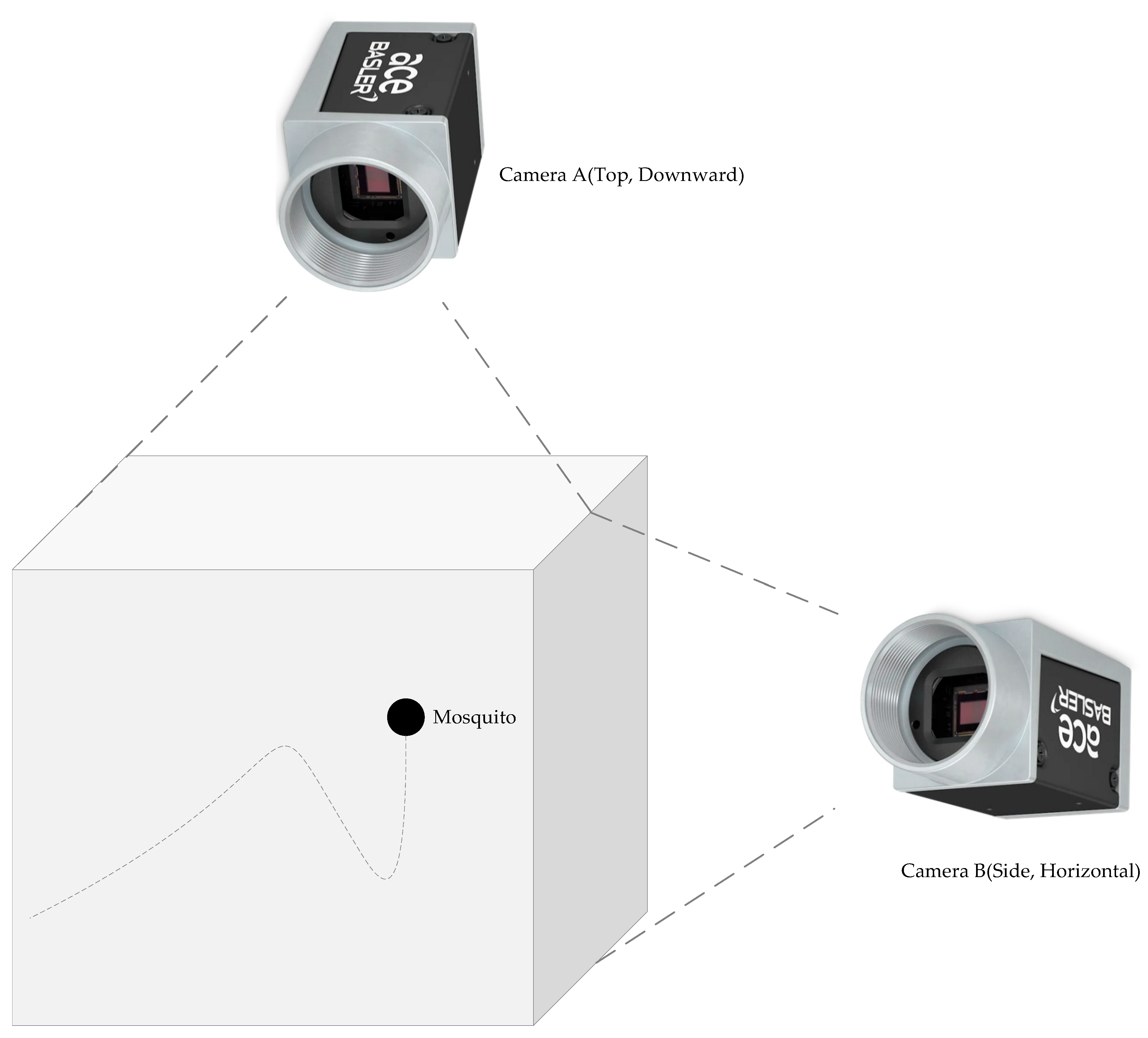
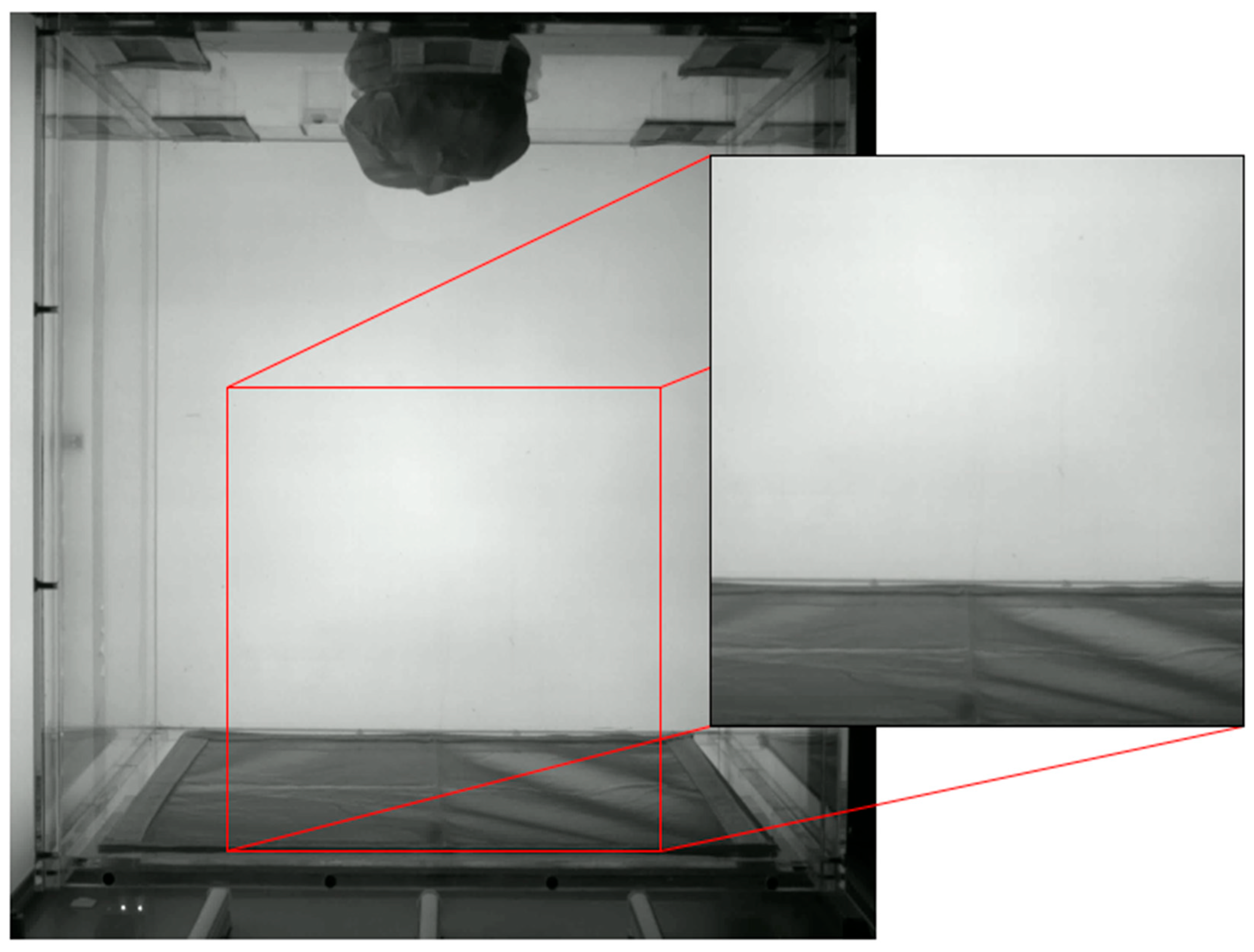
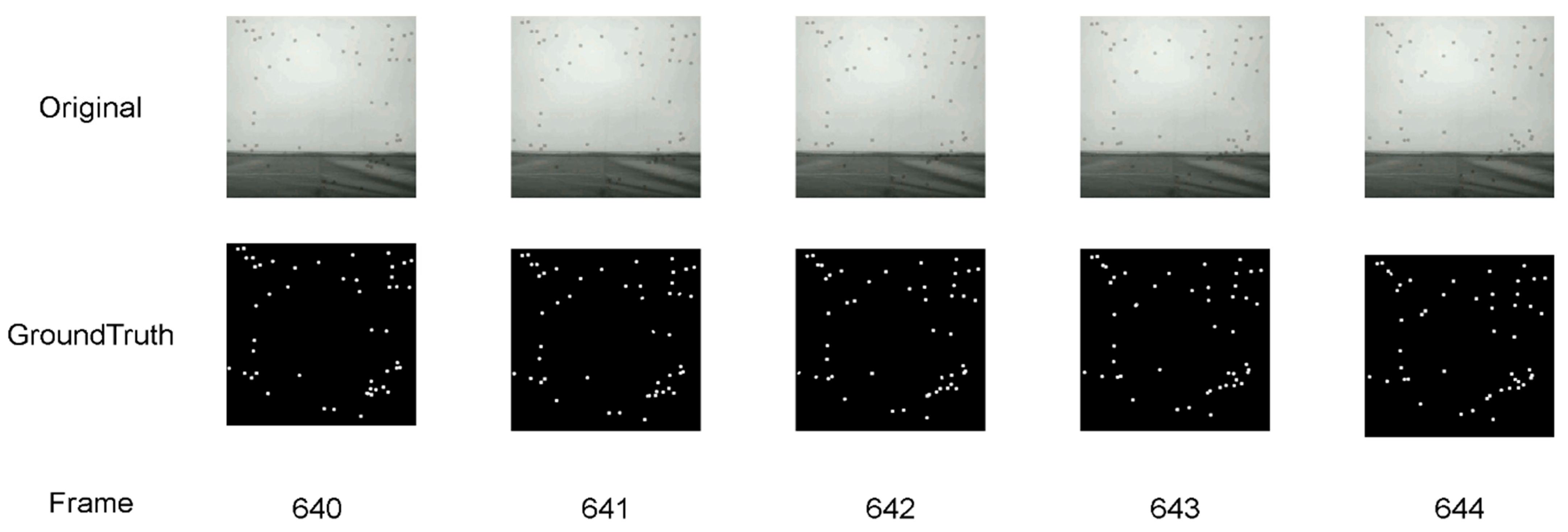
4.1.1. Experimental Scenario and Dataset Construction

The experimental setup, as illustrated in Figure 6, was designed to facilitate precise observation and analysis of mosquito flight behavior. The experiments were conducted within a transparent acrylic box (60 × 60 × 60 cm³), whose size was verified through pre-experiments to ensure sufficient space for the free flight of adult Asian tiger mosquitoes.

To achieve high-resolution imaging of mosquito movements, we employed Basler acA2000-50gm industrial cameras(Basler AG, An der Strusbek 60–62, 22926 Ahrensburg, Germany) equipped with zoom lenses, providing an imaging resolution of 0.05 mm/pixel. This resolution allows for the capture of sub-pixel movement characteristics, which are crucial for accurate trajectory reconstruction. Environmental conditions were strictly controlled, with the temperature maintained at 20 ± 1 °C, humidity at 40%, and illumination at 500 Lux. All experiments were conducted in a dark room to eliminate external light interference and ensure consistent imaging quality.

The experimental setup incorporated two cameras positioned at mutually orthogonal angles to capture mosquito flight from different perspectives.

Camera A (top placement): Positioned at the top center of the acrylic box, with its optical axis directed vertically downward.

Camera B (side placement): Mounted on the side, with its optical axis aligned horizontally, perpendicular to Camera A. This configuration ensures comprehensive coverage of mosquito movement along both the vertical and horizontal axes.

To ensure accurate trajectory reconstruction, each camera was calibrated using a standard calibration board, allowing us to determine both intrinsic and extrinsic camera parameters. Spatial markers at known distances were used to verify calibration accuracy, and systematic distortion correction parameters were applied to compensate for potential image distortion caused by rapid mosquito flight. Additionally, rigorous preprocessing steps were implemented prior to target detection and tracking to enhance the robustness of the acquired data.

Additionally, to simulate complex real-world detection scenarios, we meticulously designed a low-contrast experimental environment within the controlled chamber, as depicted in Figure 7. Specifically, internal surfaces and components were deliberately coated with a dark color palette, closely matching the coloration of the mosquito subjects. This configuration significantly increases the challenge of distinguishing mosquito targets from the background, effectively replicating detection difficulties encountered in real-world conditions characterized by low visual contrast. Consequently, this experimental setup uniquely enables rigorous evaluation and validation of algorithm robustness against visual interference in complex tracking scenarios.

To accurately evaluate the performance of the algorithms, the primary task is to construct a high-precision ground-truth dataset. This study utilizes a semi-automatic annotation tool (LabelMe v3.16) to perform pixel-by-pixel segmentation on the original video frames, thereby generating binary mask data and ensuring that all foreground target pixels are correctly segmented. However, in natural videos, the distribution of moving targets is relatively sparse, resulting in the number of background pixels being far greater than that of foreground pixels. This data skew significantly affects the reliability of evaluation metrics.

To effectively address this issue, this study innovatively introduces a data augmentation method based on artificial target synthesis, aiming to reasonably adjust the ratio of foreground-to-background targets. In the process of generating artificial targets, a 1024 × 1024 pixel region at the center of the bottom of the experimental chamber is selected as the background image. The distribution of this region in the HSV color space has a mean value of ${\sigma }_x=3.5\pm 0.3$ and a standard deviation of $\sigma =[5,3,10]$, which can effectively represent a typical low-contrast background. Meanwhile, a two-dimensional anisotropic Gaussian kernel function is used:

$$G(x,y)={\displaystyle \frac{1}{2\pi {\sigma }_x{\sigma }_y}}\exp \left(-{\displaystyle \frac{{(x-{\mu }_x)}^2}{2{\sigma }_x^2}}-{\displaystyle \frac{{(y-{\mu }_y)}^2}{2{\sigma }_y^2}}\right)$$

(17)

This function is used to simulate mosquito targets. The parameters of the kernel function are set as ${\sigma }_x=3.5\pm 0.3$ (major axis) and ${\sigma }_y=1.2\pm 0.2$ (minor axis). By appropriately perturbing these parameters, targets with various shapes are generated. In addition, the position and motion direction of the targets are randomly initialized within the background substrate, and their motion is strictly limited to this region.

After obtaining the background image, this frame is duplicated and synthesized into a video sequence containing only the background. For the mosquito targets in the original video, which are essentially ellipsoidal targets without distinct appearance features, a two-dimensional Gaussian kernel function is used to represent such targets. Within a certain range, the standard deviation of the Gaussian kernel function, the number and size of the generated artificial targets, as well as their initial velocity, position, and angle, are randomly selected. Gaussian noise is also applied to simulate the appearance of artificial mosquito targets.

Taking a single target as an example, if an artificial mosquito target is added to the video frame at time t, and its velocity and motion angle at time t − 1 are known, the velocity at time t is calculated as $v_t=v_{t-1}+{△}_v$, where $v_t$ is a velocity offset following a normal distribution. Similarly, the motion angle at time t is ${\theta }_t={\theta }_{t-1}+{△}_{\theta }$, with ${\theta }_t$ being an angular offset from a normal distribution. These offsets introduce random variations to the motion parameters. After determining the velocity and angle for the next frame, they are projected onto the x and y axes to calculate the position at the next time step. If the position exceeds the background image boundaries, the target is not added.

When adding artificial targets, their pixel values are used as the transparency channel to achieve pixel blending with the background frame. Based on the transparency of the mosquito target, each pixel is determined to retain the background or adopt the artificial target pixel value. When the transparency is close to 0, the background dominates, and when it is close to 1, the artificial target dominates, thereby superimposing the artificial mosquito target onto the background. During the superimposition process, ground-truth images are generated for subsequent algorithm performance evaluation. The generated video images and ground-truth images are shown in Figure 8.

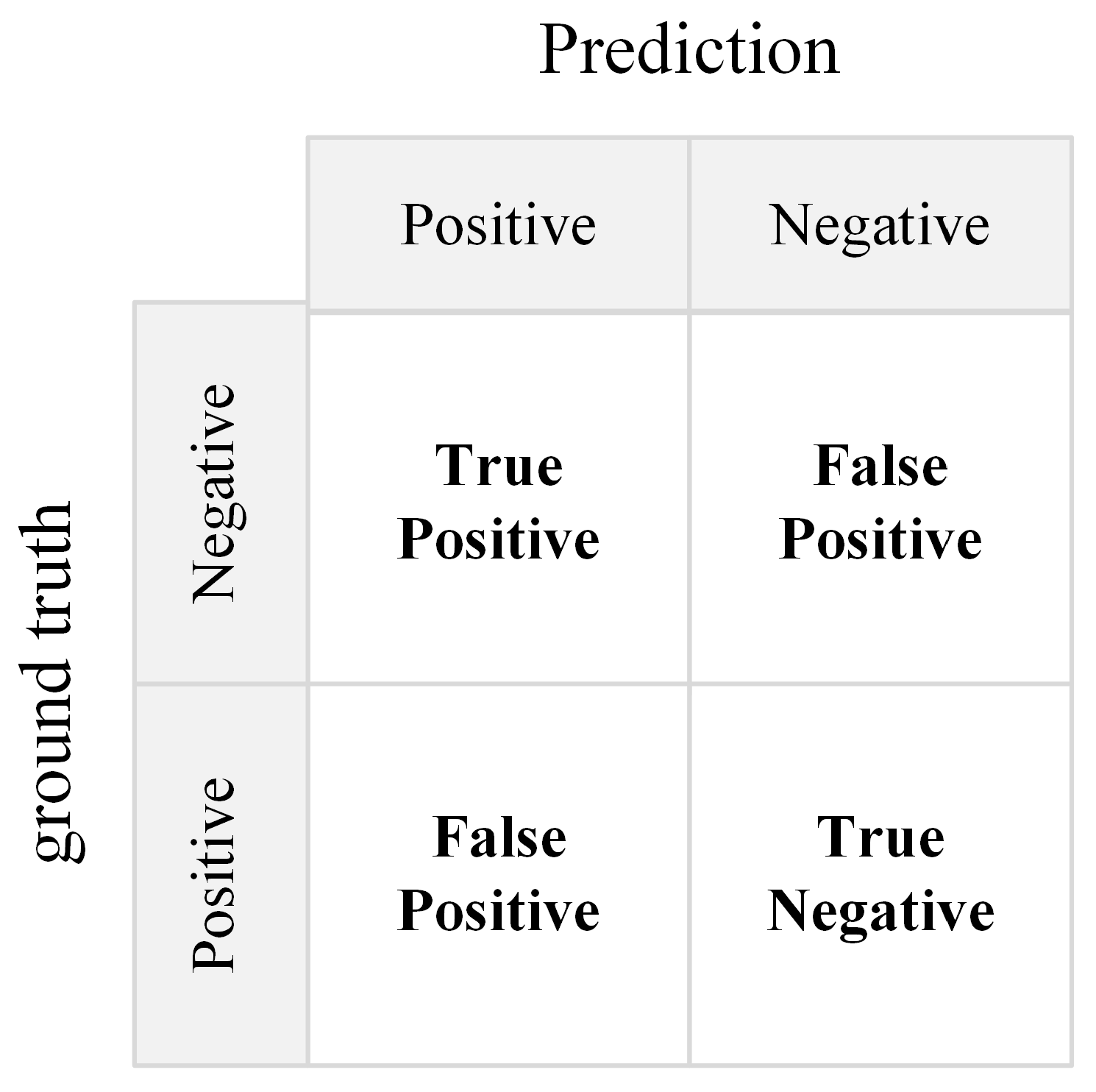
4.1.2. Experimental Metrics

Moving target detection is essentially a binary classification problem between foreground and background, analogous to the task of a classifier, which maps actual conditions to predicted categories to distinguish foreground from background. When applying background subtraction algorithms to real-world scenarios, the following four outcome classifications exist:

True Positive (TP): The target is actually foreground and is correctly identified as foreground by the algorithm.

False Negative (FN): The target is actually foreground but is mistakenly identified as background by the algorithm.

True Negative (TN): The target is actually background and is correctly identified as background by the algorithm.

False Positive (FP): The target is actually background but is mistakenly identified as foreground by the algorithm.

Given a background subtraction algorithm and test data, a 2 × 2 confusion matrix can be constructed. This matrix visually presents the algorithm’s identification results and serves as the foundation for numerous algorithm performance evaluation metrics. As shown in Figure 9, the main diagonal elements of the matrix represent correct identifications, while the off-diagonal elements correspond to incorrect identifications.

Based on the confusion matrix, the following key performance metrics can be calculated.

Precision: It refers to the proportion of correctly identified foreground targets to the total number of samples. A higher value indicates stronger recognition capability. The formula is as follows:

$$\mathrm{Precision}={\displaystyle \frac{TP}{TP+FP}}$$

(18)

Accuracy: It refers to the proportion of correctly classified samples among all samples, comprehensively reflecting the algorithm’s ability to identify both foreground and background. This metric is more effective when the proportions of foreground and background samples are similar. The formula is as follows:

$$\mathrm{Accuracy}={\displaystyle \frac{TP+TN}{P+N}}$$

(19)

Recall: If refers to the proportion of correctly identified foreground targets to the total number of foreground targets. A higher value indicates fewer missed detections, but excessively high recall may lead to misclassifying background as foreground. The formula is as follows:

$$\mathrm{Recall}={\displaystyle \frac{TP}{P}}$$

(20)

F1: It refers to a harmonic mean of precision and recall, suitable for samples with imbalanced foreground and background proportions. A higher value indicates a better balance between precision and recall. The formula is as follows:

$$\mathrm{F}1={\displaystyle \frac{2}{1/\mathrm{Precision}+1/\mathrm{Recall}}}$$

(21)

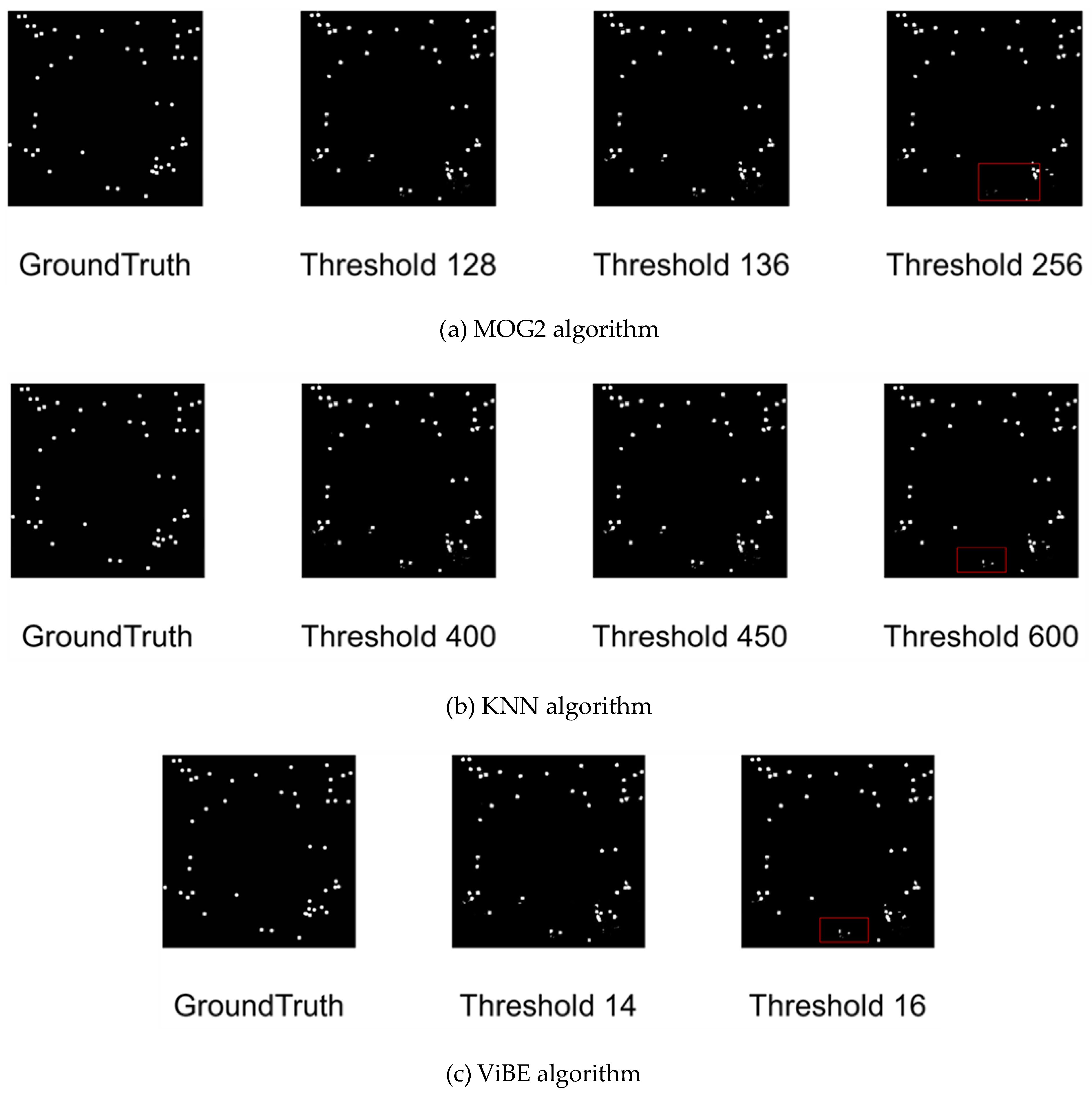
4.2. Performance Comparison of Background Subtraction Algorithms

In the background subtraction algorithm, the segmentation threshold between the foreground and background significantly affects the performance of the algorithm. To address this issue, this study employs the Receiver Operating Characteristic (ROC) analysis method [27] to determine the optimal threshold and screen for the best-performing algorithm.

The experimental data are video sequences obtained by generating artificial mosquito targets. This sequence includes video content with mosquitoes and real-world video images. Each pixel in each frame can be clearly segmented into two categories: foreground and background. Considering that mosquitoes move relatively fast and have large position changes in real-world scenarios, to accurately evaluate the performance of the algorithm under fast-moving conditions and effectively eliminate the interference of noise and random factors, this study specifically selects a short range of consecutive frames (frames 640–644) for background subtraction operations and conducts an in-depth analysis of their average values. The selected frame images and their corresponding real-world images are shown in Figure 10.

In ROC analysis, the first step is to calculate the confusion matrix of a certain frame of the image, that is, by comparing the segmentation results of the detected image and the real-world image, traversing the pixels to calculate the confusion matrix, true positive rate (TPR), and false positive rate (FPR), and then constructing the ROC curve. The ROC curve has TPR on the y-axis and FPR on the x-axis, demonstrating the trade-off between TPR and FPR at different thresholds. Generally, the closer the corresponding point of an algorithm on the ROC curve is to the upper-left corner, the better its performance. At the diagonal line, TPR is equal to FPR, indicating that the performance is equivalent to random segmentation. Algorithms in the lower-triangular region perform worse. The point (0, 1) corresponds to a perfect algorithm with a false detection rate of 0. By changing the threshold, multiple different points of the same algorithm can be obtained on the ROC curve, and connecting these points forms a complete ROC curve to determine the optimal threshold.

The experimental results are as follows: Figure 11 shows the ROC curves of three different algorithms within their respective different threshold ranges; Figure 12 presents the detection results of multiple algorithms under different threshold settings, where the real-world images are marked with red boxes to visually represent the missed detection cases.

For the MOG2 algorithm, the parameter corresponding to the threshold is varThreshold. According to the preliminary threshold ROC curve in Figure 11a, when the threshold is set to 128, the average true positive rate is approximately 0.95; when the threshold is increased to 256, the average true positive rate drops to about 0.90. Further observation reveals that when the threshold is greater than 256, a significant decrease in the true positive rate is needed to obtain a very limited decrease in the false positive rate. Based on this, the reasonable range for threshold selection should be determined within $\left[128,256\right]$. A careful examination of the ROC curve within this threshold range shows that when the threshold is 136, the true positive rate reaches the highest level, and the false positive rate is relatively low. If the threshold is further increased, it will not bring significant benefits and may increase the potential risk of missed detection. In addition, as shown in Figure 12a, when the threshold is set to 136, no missed detection occurs. Taking all these factors into account, 136 is finally determined as the significant threshold for the MOG2 algorithm in the current scenario.

For the KNN algorithm, the parameter corresponding to the threshold is dist2Threshold. As can be seen from the preliminary threshold ROC curve in Figure 11b, when the threshold is 400, the corresponding average true positive rate is approximately 0.95; when the threshold is increased to 600, the average true positive rate is about 0.91. During the process of increasing the threshold from 0 to 400, only a very small sacrifice of the true positive rate is required to achieve a significant decrease in the false positive rate. However, when the threshold exceeds 600, the effect of reducing the false positive rate weakens sharply. Therefore, in order to obtain relatively ideal algorithm performance, the reasonable value range of the threshold should be within $\left[400,600\right]$. An in-depth analysis of the ROC curve within this threshold range shows that when the threshold is increased to 450, only a very small sacrifice of the true positive rate is needed to achieve a relatively large decrease in the false positive rate. At the same time, as shown in Figure 12b, when the threshold is set to 450, no missed detection occurs. Based on the above analysis, 450 can be determined as the significant threshold for the KNN algorithm in background subtraction in this application scenario.

For the ViBe algorithm, the parameter corresponding to the threshold is Distance Threshold. According to the preliminary threshold ROC curve in Figure 11c, when the threshold is 14, the average true positive rate is approximately 0.95; when the threshold is changed to 16, the average true positive rate is about 0.91. When the threshold is greater than 16, a relatively large decrease in the true positive rate is also required to obtain a poor decrease in the false positive rate. In view of this, the reasonable range for threshold selection should be within $\left[14,16\right]$. A careful observation of the ROC curve within this threshold range shows that when the threshold is 14, the true positive rate is at a relatively high level, and the false positive rate is relatively low. When the threshold is increased to 15, the decrease in the false positive rate is relatively small. In addition, as shown in Figure 12c, when the threshold is set to 14, no missed detection occurs. Considering all these factors, 14 can be determined as a significant threshold for the ViBe algorithm in background subtraction.

Subsequently, based on the detection results of each algorithm at the significant thresholds, calculations were carried out for precision rate, accuracy rate, recall rate, and F1-score. The aim is to screen out the algorithm with more prominent segmentation performance through the comparison of these metrics. The specific results are shown in

Table 1. Metric values of various algorithms.

Algorithm	Precision	Accuracy	Recall	F1-Score
MOG2	0.9167	0.9167	0.9507	0.9334
KNN	0.9106	0.9335	0.9456	0.9297
ViBe	0.9068	0.9308	0.9483	0.9270

.

From the perspective of precision rate, the precision rates of the three algorithms, namely MOG2, KNN, and ViBe, are nearly identical. The accuracy rates of KNN and ViBe are similar and both are higher than that of MOG2, which clearly indicates that KNN and ViBe have more advantages in overall segmentation accuracy. The recall rates of MOG2, KNN, and ViBe are relatively close, suggesting that these three algorithms can effectively reduce missed detections when detecting foreground objects and identify foreground objects as comprehensively as possible. When considering the F1-score, MOG2 exhibits the highest F1-score, which means that on the basis of ensuring the precision rate, MOG2 has a stronger ability to detect more foreground objects.

In addition, the background modeling time window also affects the detection results. When a longer time window is used for background modeling, the model tends to be stable due to the slow pixel changes in historical frames. If a fast-moving object enters, the algorithm may not be able to adapt to the rapid changes and thus mistakenly identify the foreground object as the background.

To evaluate the computational complexity of these algorithms, we conducted experiments using three video sequences of different lengths: 100 frames, 1000 frames, and 10,000 frames. Each experiment was repeated five times, and the average processing time was used as the main metric. The results are shown in Figure 13. Specifically, the average processing speed of ViBe is approximately 5.5 frames per second, that of MOG2 is about 6 frames per second, and that of KNN is around 13 frames per second.

Taking both computational complexity and performance metrics into account, the KNN algorithm has a relatively fast processing speed while ensuring high accuracy and recall rate. Although MOG2 has a slightly higher F1-score, its slow processing speed may limit its practical applications. Although ViBe performs well in terms of recall rate, it has the slowest processing speed and its accuracy is lower than that of KNN. Therefore, considering the segmentation performance and computational efficiency of the algorithms, it is reasonable to choose the KNN algorithm as the object segmentation algorithm. The KNN algorithm provides a good balance among accuracy, recall rate, and processing speed, and can meet the requirements for segmentation performance and computational efficiency in practical applications.

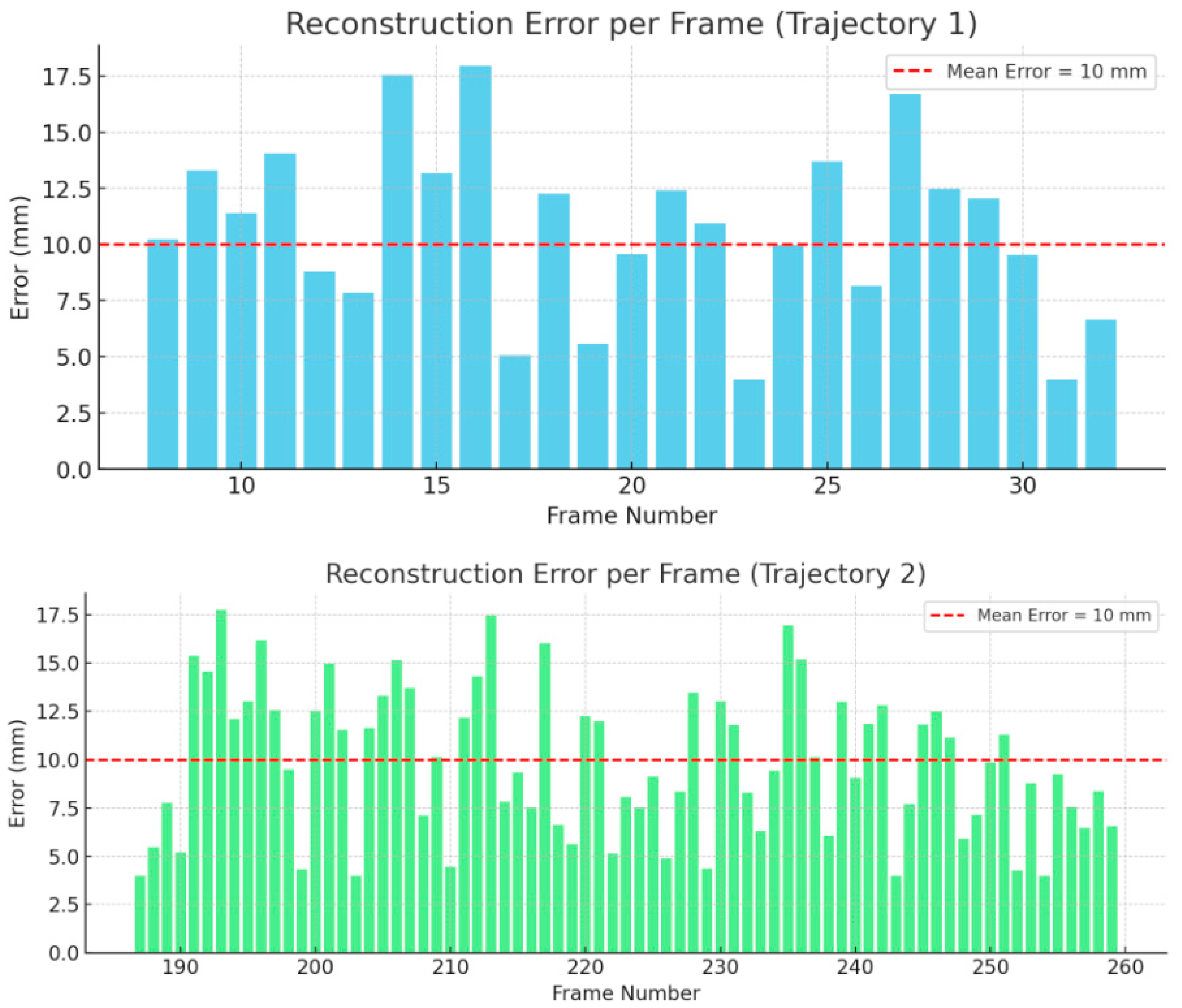
4.3. Trajectory Screening and 3D Trajectory Reconstruction for Dim-Point Mosquito Targets

In video-based foreground object detection, once the binary segmentation of foreground and background is obtained, it is essential to accurately localize the mosquito targets for subsequent tracking. This involves determining the centroid coordinates by extracting contours and bounding boxes.

Figure 14 illustrates the process of object localization. The raw binary image obtained using background subtraction algorithms, such as KNN, often contains noise points that interfere with tracking, as shown in Figure 14b. To mitigate this, a morphological opening operation (erosion followed by dilation) is applied to remove small noise while preserving the object shape, resulting in a cleaner foreground image (Figure 14c).

Contours of the foreground objects are then extracted through image connectivity analysis, distinguishing between foreground and background pixels based on four-neighborhood or eight-neighborhood connectivity rules. The resulting contours (marked in red) are shown in Figure 14d.

Once the contours are obtained, bounding boxes are drawn using OpenCV’s boundingRect() function, followed by boundary checks to prevent out-of-frame detections. The centroid coordinates are computed from the contour’s image moments, as shown in Figure 14e, where green boxes represent detected objects, and red circles indicate their centroids.

After obtaining centroid coordinates, Kalman filtering is applied to refine trajectory tracking by predicting and updating object motion. Figure 15 demonstrates an example frame where Kalman filtering is used to estimate the mosquito’s movement. In this figure, the green box represents the object’s bounding box; the red circle denotes the observed centroid; the blue circle indicates the predicted position before update; and the yellow circle marks the corrected estimation after update.

In multi-object tracking, the motion detector identifies moving targets but does not inherently distinguish between different individuals. To maintain object identity across frames, we employ the Hungarian matching algorithm for target association. This ensures consistent tracking of each mosquito, even in dense or overlapping trajectories.

Figure 16 presents the multi-frame trajectory tracking results of low-visibility mosquito targets captured using an orthogonal dual-camera system. It demonstrates the robustness of the tracking algorithm in preserving trajectory continuity and maintaining stable object identities in complex scenes. Additionally, through multi-frame comparisons, the algorithm’s ability to track dynamically moving targets consistently is validated.

During tracking, unreliable or erroneous trajectories may still arise due to detection noise, occlusions, or limitations in detector performance. Therefore, before incorporating trajectories into the final analysis, a screening process is necessary to filter out invalid or inconsistent tracks.

The first step in trajectory screening involves frame alignment and preprocessing. Due to potential initialization delays in background subtraction algorithms, the first few frames may exhibit asynchrony between different video sequences. To correct this, frames are aligned, and mismatched data points are removed. Additionally, since tracking results from different frames may vary in continuity, a minimum trajectory length threshold is applied—filtering out short-lived trajectories that are unlikely to represent actual mosquito motion. Once filtered, the three-dimensional trajectory reconstruction is performed using the coordinate transformation model.

Object tracking is carried out on the video sequences of the movement of mosquito objects simultaneously captured by two orthogonal cameras. The obtained coordinates and the converted three-dimensional trajectory coordinates are shown in

Table 2. Coordinate conversion values of Trajectory 1 (unit: pixel).

Frame	xv	yv	xh	yh	x	y	z
8	1402	1404	352	1622	877	1404	1622
9	1403	1415	334	1621	869	1415	1621
10	1405	1425	317	1622	861	1425	1622
11	1412	1436	301	1621	857	1436	1621
…	…	…	…	…	…	…	…
27	1554	1508	165	1701	860	1508	1701
28	1562	1517	160	1719	861	1517	1719
29	1571	1530	156	1738	864	1530	1738
30	1582	1535	151	1757	867	1535	1757
31	1596	1529	147	1743	872	1529	1743
32	1608	1521	152	1737	880	1521	1737

and

Table 3. Coordinate conversion values of Trajectory 2 (unit: pixel).

Frame	xv	yv	xh	yh	x	y	z
187	1288	328	1645	1529	1467	328	1529
188	1286	310	1654	1514	1470	310	1514
189	1287	295	1662	1499	1475	295	1499
190	293	280	1671	1484	1482	280	1484
…	…	…	…	…	…	…	…
254	899	1242	576	1711	738	1242	1711
255	884	1253	563	1721	724	1253	1721
256	870	1261	553	1737	712	1261	1737
257	861	1265	549	1745	705	1265	1745
258	859	1263	552	1736	706	1263	1736
259	856	1259	559	1722	708	1259	1722

. Based on the trajectory coordinates, the 3D trajectory reconstruction results are presented in Figure 17 and Figure 18, where Table 2 corresponds to Trajectory 1 (used to validate algorithm performance under typical scenarios, including straight flights and gradual turns) and Table 3 corresponds to Trajectory 2 (used to evaluate robustness against dynamic challenges such as rapid accelerations/decelerations and complex spatial maneuvers).

In the table, the 3D coordinates x, y, and z are recorded in pixels. These values are derived from the 2D pixel coordinates $x_v, y_v$ (vertical camera, Camera A) and $x_h, y_h$(horizontal camera, Camera B) via the transformation formulas: $x={\displaystyle \frac{x_v+x_h}{2}}$, $y=y_v$, $z=y_h$.

To validate the physical spatial accuracy, a calibration factor of $0.05 \mathrm{mm}/\mathrm{pixel}$ was applied to convert pixel coordinates to millimeters. The average reconstruction error of the 3D trajectories was $10\pm 4 \mathrm{mm}$.

In the figure, the green dot marks the trajectory starting point. The upper-left panel displays the 3D trajectory reconstruction result, the middle-left and middle-right panels show the projections onto the XOY and YOZ planes, respectively, and the lower-right panel presents the projection of the detected trajectory. The results demonstrate a high morphological consistency between the reconstructed and detected trajectories, effectively reflecting the actual flight paths of mosquitoes.

To further validate the 3D trajectory reconstruction accuracy stated in the abstract, we analyzed the frame-by-frame spatial deviation between the reconstructed points and their corresponding ground truth projections. Figure 19 presents the per-frame reconstruction errors for Trajectory 1 (Frame 8–32) and Trajectory 2 (Frame 187–259). The results show that the majority of errors fall within the 10 ± 4 mm range, with mean errors of 10.2 mm and 9.8 mm, respectively. These values confirm that the proposed system achieves consistent millimeter-level reconstruction accuracy across different motion patterns and temporal segments.

5. Discussion

This study presents an innovative framework for reconstructing three-dimensional mosquito flight trajectories, integrating background subtraction, multi-target tracking, and stereo vision. By addressing the critical challenges in detecting and tracking small, fast-moving targets, this approach marks a significant advancement over traditional two-dimensional methodologies. Utilizing optimized KNN-based background subtraction, Kalman filtering with elliptical weighting, and orthogonal binocular vision, the system achieves high-precision 3D trajectory reconstruction with a mean error of 10 ± 4 mm, outperforming previous studies in both accuracy and real-time performance.

The optimized KNN background subtraction algorithm exhibits superior performance in sub-pixel mosquito target detection compared to conventional methods like MOG2 and ViBe. Experimental results reveal that KNN balances precision (0.91), recall (0.94), and processing speed (13 FPS), surpassing MOG2 (F1-score: 0.93) and ViBe (F1-score: 0.93) under low-contrast conditions. While aligning with Zivkovic and Van Der Heijden’s [14] findings on KNN’s adaptability to complex scenes, this study extends their work by validating its efficacy in micro-target detection.

In multi-target tracking, the integration of Kalman filtering with elliptical weighting and the Hungarian algorithm-based data association enhances trajectory continuity significantly. By modeling predicted target positions as ellipses and adjusting matching costs based on positional likelihood, the system mitigates issues such as identity switches and trajectory fragmentation. As illustrated in Figure 4, this approach outperforms traditional Euclidean distance-based association methods, especially for high-speed, maneuverable targets.

The orthogonal binocular vision model for 3D reconstruction represents a critical advancement over prior stereo vision systems. With a reconstruction error of 10 ± 4 mm, this method surpasses the 3D tracking accuracy reported by Khan et al. [21] (mean error: 15 mm) and Cheng et al. [22,23] (mean error: 12 mm), enabling detailed analysis of mosquito flight dynamics.

Although deep learning-based methods like Mask R-CNN [8] achieve high detection accuracy for larger targets, their performance diminishes significantly on sub-pixel mosquito imagery due to limited feature extractability. Conversely, the proposed KNN-based approach maintains robustness under low-contrast and high-speed conditions, despite slightly lower precision. This trade-off between accuracy and computational efficiency renders the method more suitable for real-time applications in resource-constrained environments.

Regarding multi-target tracking, SORT and DeepSORT [18,19], which rely on appearance features and CNN-based embeddings, prove ineffective for textureless mosquito targets. The elliptical weighting strategy in this study compensates for the absence of appearance features by emphasizing motion continuity, achieving comparable tracking stability without the overhead of deep learning.

For 3D trajectory reconstruction, commercial solutions like Track3D [10,11] require specialized wind tunnel setups and extensive calibration, limiting field applicability. The proposed orthogonal vision system simplifies calibration by assuming aligned optical axes, reducing setup complexity while maintaining high accuracy.

Notwithstanding these advancements, several limitations merit further investigation. The KNN algorithm’s performance in dynamic outdoor environments remains untested, as evidenced by its sensitivity to illumination changes and background clutter. Integrating lightweight CNN models optimized for micro-targets could enhance robustness in complex scenarios. Additionally, the linear Kalman filter’s inability to handle abrupt accelerations or non-linear flight patterns introduces prediction errors. Transitioning to non-linear models, such as the unscented Kalman filter (UKF) or particle filters [16], could improve trajectory estimation, particularly during erratic maneuvers.

Furthermore, the stereo vision system’s reliance on fixed, orthogonal cameras restricts scalability. Future research should explore multi-camera networks with adaptive calibration, as proposed by Straw et al. [17], to enable 3D tracking in larger, unstructured environments. Incorporating depth sensors (e.g., LiDAR) or event-based cameras could further enhance reconstruction accuracy and temporal resolution.

The framework’s generalizability extends beyond mosquito research. Its modular design supports adaptation to other fast-flying insects, such as fruit flies or agricultural pests, through adjustments to motion models and camera configurations. This aligns with emerging trends in ecological monitoring and precision agriculture, where high-precision tracking tools are pivotal for understanding species interactions and optimizing pest control strategies.

6. Conclusions

This study presents a novel framework for 3D trajectory reconstruction of mosquito flight behavior, integrating motion detection, multi-target tracking, and binocular vision techniques. The proposed method achieves >95% detection accuracy with an F1-score of 0.93, and the 3D reconstruction error remains within millimeter-level precision, significantly improving upon traditional 2D tracking methods. The experimental validation demonstrates that the system maintains stable trajectory tracking and identity association even under low-visibility conditions, highlighting its robustness in complex environments.

The reconstructed high-precision flight trajectories provide valuable insights into mosquito movement patterns, offering direct support for research on vector control strategies, host-seeking behavior, and pest management applications. By capturing fine-scale motion dynamics, this framework enables a more detailed understanding of mosquito spatial behavior, which is essential for developing targeted intervention strategies in public health and agriculture.

Future work will focus on extending this approach to multi-species tracking, optimizing computational efficiency for real-time deployment, and integrating multi-modal sensing techniques to enhance environmental adaptability. These advancements will further broaden the applicability of this framework in biological research, ecological monitoring, and applied entomology.

References

1. Vaidya, N.K.; Wang, F.-B. Persistence of Mosquito Vector and Dengue: Impact of Seasonal and Diurnal Temperature Variations. Discret. Contin. Dyn. Syst.-B 2021, 27, 393–420. [Google Scholar] [CrossRef]
2. Wang, Y.; Li, Y.; Ren, X.; Liu, X. A periodic dengue model with diapause effect and control measures. Appl. Math. Model. 2022, 108, 469–488. [Google Scholar]
3. Omari, G. Study of Effects of Plasmodium Infections on the Lifespan of Female Anopheles Mosquitoes. Master’s Thesis, Harvard University, Cambridge, MA, USA, 2018. [Google Scholar]
4. Dragovic, S.M.; Agunbiade, T.A.; Freudzon, M.; Yang, J.; Hastings, A.K.; Schleicher, T.R.; Zhou, X.; Craft, S.; Chuang, Y.M.; Gonzalez, F.; et al. Immunization with AgTRIO, a Protein in Anopheles Saliva, Contributes to Protection against Plasmodium Infection in Mice. Cell Host Microbe 2018, 23, 523–553. [Google Scholar] [CrossRef] [PubMed]
5. Jeong, C.; Song, J.S.; Kim-Jeon, M.D.; Kim, K.H.; Lee, J.G.; Lee, S.M. Molecular survey of Dirofilaria immitis in mosquitoes collected from parks the in the Incheon metropolitan city in Korea. Korean J. Vet. Serv. 2020, 43, 1–6. [Google Scholar]
6. Şuleşco, T.; Volkova, T.; Yashkova, S.; Tomazatos, A.; von Thien, H.; Lühken, R.; Tannich, E. Detection of Dirofilaria repens and Dirofilaria immitis DNA in mosquitoes from Belarus. Parasitol. Res. 2016, 115, 3677. [Google Scholar] [PubMed]
7. Vo-Doan, T.T.; Straw, A.D. Videography using a fast lock on, gimbal-mounted tracking camera to study animal communication. In Integrative and Comparative Biology; Oxford Univ Press Inc.: Cary, NC, USA, 2001; Volume 61, p. E949. [Google Scholar]
8. Javed, N.; Paradkar, P.N.; Bhatti, A. Flight behaviour monitoring and quantification of aedes aegypti using convolution neural network. PLoS ONE 2023, 18, e0284819. [Google Scholar]
9. Wang, J.T.; Bu, Y. Internet of Things-based smart insect monitoring system using a deep neural network. IET Netw. 2022, 11, 245–256. [Google Scholar]
10. Spitzen, J.; Spoor, C.W.; Grieco, F.; ter Braak, C.; Beeuwkes, J.; van Brugge, S.P.; Kranenbarg, S.; Noldus, L.P.J.J.; van Leeuwen, J.L.; Takken, W. A 3D analysis of flight behavior of Anopheles gambiae sensu stricto malaria mosquitoes in response to human odor and heat. PLoS ONE 2013, 8, e62995. [Google Scholar]
11. Spitzen, J.; Takken, W. Keeping track of mosquitoes: A review of tools to track, record and analyse mosquito flight. Parasites Vectors 2018, 11, 1–11. [Google Scholar]
12. Zivkovic, Z. Improved adaptive Gaussian mixture model for background subtraction. In Proceedings of the 17th International Conference on Pattern Recognition, 2004. ICPR 2004, Cambridge, UK, 26 August 2004; Volume 2, pp. 28–31. [Google Scholar]
13. Barnich, O.; Van Droogenbroeck, M. ViBe: A universal background subtraction algorithm for video sequences. IEEE Trans. Image Process. 2010, 20, 1709–1724. [Google Scholar] [PubMed]
14. Zivkovic, Z.; Van Der Heijden, F. Efficient adaptive density estimation per image pixel for the task of background subtraction. Pattern Recognit. Lett. 2006, 27, 773–780. [Google Scholar] [CrossRef]
15. Welch, G.; Bishop, G. An Introduction to the Kalman Filter; University of North Carolina at Chapel Hill: Chapel Hill, NC, USA, 1995. [Google Scholar]
16. Chen, X.; Wang, X.; Xuan, J. Tracking multiple moving objects using unscented Kalman filtering techniques. arXiv 2018, arXiv:1802.01235. [Google Scholar]
17. Straw, A.D.; Pieters, R.; Muijres, F.T. Real-Time Tracking of Multiple Moving Mosquitoes. Cold Spring Harb. Protoc. 2022, 2023, 117–120. [Google Scholar] [CrossRef] [PubMed]
18. Wojke, N.; Bewley, A.; Paulus, D. Simple online and realtime tracking with a deep association metric. In Proceedings of the 2017 IEEE International Conference on Image Processing (ICIP), Beijing, China, 17–20 September 2017; pp. 3645–3649. [Google Scholar]
19. Bewley, A.; Ge, Z.; Ott, L.; Ramos, F.; Upcroft, B. Simple online and realtime tracking. In Proceedings of the 2016 IEEE International Conference on Image Processing (ICIP), Phoenix, AZ, USA, 25–28 September 2016; pp. 3464–3468. [Google Scholar]
20. Kuhn, H.W. The Hungarian method for the assignment problem. Nav. Res. Logist. Q. 1955, 2, 83–97. [Google Scholar] [CrossRef]
21. Khan, B.; Gaburro, J.; Hanoun, S.; Duchemin, J.B.; Nahavandi, S.; Bhatti, A. Activity and flight trajectory monitoring of mosquito colonies for automated behaviour analysis. In Neural Information Processing: 22nd International Conference, ICONIP 2015, November 9–12, 2015, Proceedings, Part IV 22; Springer International Publishing: Cham, Switzerland, 2015; pp. 548–555. [Google Scholar]
22. Cheng, X.E.; Wang, S.H.; Qian, Z.M.; Chen, Y.Q. Estimating Orientation of Flying Fruit Flies. PLoS ONE 2015, 10, e0132101. [Google Scholar]
23. Cheng, X.E.; Qian, Z.M.; Wang, S.H.; Jiang, N.; Guo, A.; Chen, Y.Q. A novel method for tracking individuals of fruit fly swarms flying in a laboratory flight arena. PLoS ONE 2015, 10, e0129657. [Google Scholar]
24. Yang, B.; Nevatia, R. Multi-target tracking by online learning of non-linear motion patterns and robust appearance models. In Proceedings of the 2012 IEEE Conference on Computer Vision and Pattern Recognition, Providence, RI, USA, 16–21 June 2012; pp. 1918–1925. [Google Scholar]
25. Li, X.R.; Jilkov, V.P. Survey of maneuvering target tracking. Part I. Dynamic models. IEEE Trans. Aerosp. Electron. Syst. 2003, 39, 1333–1364. [Google Scholar]
26. Reece, S.; Roberts, S. The near constant acceleration Gaussian process kernel for tracking. IEEE Signal Process. Lett. 2010, 17, 707–710. [Google Scholar]
27. Fawcett, T. An introduction to ROC analysis. Pattern Recognit. Lett. 2006, 27, 861–874. [Google Scholar]
Figure 1. Flowchart of the background subtraction algorithm based on k-nearest neighbor.
Electronics 14 01333 g001
Figure 2. Multi-target association workflow using hungarian algorithm with the Kalman filter prediction (the green-filled area represents the matching results).
Electronics 14 01333 g002
Figure 3. Cost matrix construction for data association: the Euclidean distance (px) between detected objects (M3, M4) and tracked objects (M1, M2) with velocity-adaptive elliptical weighting (R < 1.0).
Electronics 14 01333 g003
Figure 4. Elliptical representation of target position and velocity predicted by the Kalman filter.
Electronics 14 01333 g004
Figure 5. Schematic of the orthogonal dual-camera system for 3D trajectory reconstruction.
Electronics 14 01333 g005
Figure 6. Schematic diagram of the experimental system setup.
Electronics 14 01333 g006
Figure 7. Schematic of the experimental setup and designated data region within a 60 × 60 × 60 cm3 transparent acrylic chamber (low-contrast environment).
Electronics 14 01333 g007
Figure 8. Example of generated data and corresponding ground-truth images based on synthetic artificial targets.
Electronics 14 01333 g008
Figure 9. Construction of confusion matrix and derivation of performance metrics for background subtraction algorithm.
Electronics 14 01333 g009
Figure 10. Example images of frames 640–644 for the performance testing of the background subtraction algorithm (including original images and ground truth images).
Electronics 14 01333 g010
Figure 11. ROC curves of diverse algorithms across varying thresholds.
Electronics 14 01333 g011
Figure 12. Comparison diagram of mosquito target detection results of various algorithms under optimal thresholds (missed detection areas marked in red).
Electronics 14 01333 g012
Figure 13. Processing efficiency comparison of MOG2, KNN, and ViBe algorithms across video sequences of different lengths.
Electronics 14 01333 g013
Figure 14. (ae) Flowchart of drawing object bounding boxes based on morphological processing and contour extraction.
Electronics 14 01333 g014
Figure 15. Schematic diagram of the prediction and update results of the movement of mosquito targets by the Kalman filter based on background subtraction and contour extraction.
Electronics 14 01333 g015
Figure 16. Multi-frame trajectory tracking of low-visibility mosquito targets in orthogonal dual-camera system (ΔT = 4 Frames): validation of tracking algorithm robustness.
Electronics 14 01333 g016
Figure 17. Comparison between the 3D trajectory reconstruction result and the tracking result of Trajectory 1.
Electronics 14 01333 g017
Figure 18. Comparison between the 3D trajectory reconstruction result and the tracking result of Trajectory 2.
Electronics 14 01333 g018
Figure 19. Per-frame 3D trajectory reconstruction error for Trajectory 1 and Trajectory 2.
Electronics 14 01333 g019