Article

UMAP-Based All-MLP Marine Diesel Engine Fault Detection Method

1
Merchant Marine College, Shanghai Maritime University, Shanghai 200135, China
2
Shanghai Ship and Shipping Research Institute, Shanghai 200135, China
3
College of Artificial Intelligence, Shenyang Aerospace University, Shenyang 110136, China
4
College of Marine Engineering, Dalian Maritime University, Dalian 116026, China
*
Authors to whom correspondence should be addressed.
Electronics 2025, 14(7), 1293; https://doi.org/10.3390/electronics14071293
Submission received: 24 February 2025 / Revised: 19 March 2025 / Accepted: 24 March 2025 / Published: 25 March 2025

Abstract

:
This study presents an innovative approach for marine diesel engine fault detection, integrating unsupervised learning through Uniform Manifold Approximation and Projection (UMAP) dimensionality reduction with time series prediction, offering significant improvements over existing methods. Unlike traditional model-based or expert-driven approaches, which struggle with complex nonlinear systems, or supervised data-driven methods limited by scarce labeled fault data, our unsupervised method establishes a normal operational baseline without requiring fault labels, enhancing applicability across diverse conditions. Leveraging UMAP’s nonlinear dimensionality reduction, the proposed method outperforms conventional linear techniques (e.g., PCA) by amplifying subtle system anomalies, enabling earlier detection of state transitions—up to two batches before deviations appear in traditional performance indicators (Ps)—thus improving fault detection sensitivity. To address nonlinear relationships in UMAP-reduced dimensions, the proposed TimeMixer-FI model enhances the TimeMixer architecture with MLP-Mixer layers. The TimeMixer-FI model demonstrates consistent improvements over the original TimeMixer across various sequence lengths, achieving an MSE reduction of 69.1% (from 0.0544 to 0.0168) and an MAE reduction of 46.3% (from 0.1023 to 0.0549) at an input sequence length of 60 time steps, thereby enhancing the reliability of the time series prediction baseline. Experimental results validate that this approach significantly enhances both the sensitivity and accuracy of early fault detection, providing a more robust and efficient solution for predictive maintenance in marine diesel engines.

1. Introduction

As industrial systems advance toward higher levels of automation, complexity, and interconnectivity, ensuring system reliability has become paramount [1]. Fault Detection and Diagnosis (FDD) technologies play a crucial role in maintaining continuous system operation by identifying and localizing faults, thereby supporting maintenance decisions [2]. Over the past decade, FDD technologies have made significant strides across various sectors, including manufacturing [3], energy systems [4], and transportation [5].
Maritime transport, as a cost-effective mode of global trade, has become increasingly vital and demonstrates promising growth potential [6]. Ships powered by marine diesel engines form the backbone of this industry. Failure to detect engine faults promptly can result in substantial economic losses and severe safety risks [7]. Diesel engine faults account for the majority of marine power system failures. Recently, with advancements in artificial intelligence and industrial big data, data-driven FDD methods have been widely adopted for marine diesel engine maintenance, becoming crucial tools for ensuring safe navigation [8]. While this study validates our unsupervised fault detection approach using marine diesel engine data, its reliance on general principles of anomaly detection and time series analysis—independent of domain-specific features—suggests potential applicability to other engineering fields, such as aerospace or manufacturing, pending validation with diverse datasets. This study implements an unsupervised FDD approach for marine diesel engines using tanker data; however, it does not involve dataset-specific feature optimization or tailored preprocessing efforts. While rooted in general anomaly detection and time series analysis principles, its applicability to other domains—such as aerospace or manufacturing—remains to be validated with diverse datasets.
In the domains of ship fault detection, traditional approaches have primarily relied on models and expert knowledge. However, as ship systems grow increasingly complex and certain vessels require unique and confidential handling, model-based methods have become progressively infeasible. The complexity and uncertainty of marine engine systems make constructing precise models nearly impossible, significantly undermining the reliability of traditional fault detection methods. Moreover, relying solely on expert knowledge poses challenges, particularly in addressing the diverse and complex nature of ship operations [9].
With the rapid advancement of artificial intelligence, these methods have shifted away from reliance on prior knowledge, instead leveraging large-scale real-world data and experience to achieve higher accuracy in fault diagnosis and detection [10]. Data-driven techniques can integrate multi-source data, overcoming traditional methods’ limitations, and have increasingly become the dominant approach in this field [11]. However, in practical applications, the high cost of acquiring and labeling fault data, coupled with the complexity and variability of fault patterns, makes supervised learning methods difficult to implement widely [12]. Unsupervised learning, which identifies anomalous states by learning system behavior patterns during normal operation, offers a new approach to addressing data scarcity [13].
Unsupervised anomaly detection approaches that establish predictive patterns from normal operation data provide an effective mechanism for identifying potential anomalies without invasive interventions. Unlike many supervised frameworks that employ physics-informed models or depend on labeled fault data, our method integrates UMAP for nonlinear dimensionality reduction and transition state extraction with TimeMixer-FI for unsupervised time series prediction. By comparing UMAP-reduced features from six correlated metrics against a seventh un-reduced metric, anomalies are detected via mode transitions without requiring fault labels. By defining a baseline of typical behavior using sensor data, deviations from this norm can be flagged as early indicators of faults, eliminating the need for labeled fault data or destructive testing. However, in high-dimensional time series data, the complexity of analysis escalates, making dimensionality reduction techniques indispensable. These methods extract critical features while reducing computational overhead, enabling proactive maintenance without compromising system integrity. Traditional approaches like Principal Component Analysis (PCA) generate orthogonal components but struggle to preserve the intrinsic structure of nonlinear data. In contrast, Uniform Manifold Approximation and Projection (UMAP) has emerged as a powerful alternative, excelling in maintaining both local and global data structures, as highlighted in [14]. This topology-preserving characteristic makes UMAP particularly suitable for fault detection in a nondestructive maintenance context, as it effectively captures system state transitions in a reduced dimensional space using only noninvasive sensor readings, a strength further emphasized in [15]. By enabling early anomaly detection without physical disruption, UMAP supports the goals of nondestructive maintenance, such as preserving equipment functionality and minimizing operational risks.
The selection of UMAP for dimensionality reduction in high-dimensional marine engine data is driven by its demonstrated superiority in handling nonlinear data structures, making it an optimal choice for fault detection in complex systems. Studies such as Altin and Cakir (2024) [16] have shown that UMAP enhances anomaly detection accuracy in multivariate time series datasets like MSL, SMAP, and SWaT, while significantly reducing training times by approximately 300–650%, owing to its ability to preserve both local and global structures. Similarly, research on structural health monitoring of damaged wind turbine blades underscores UMAP’s superior performance over PCA and t-SNE in feature extraction and classification of vibration signals, adeptly managing high-dimensional nonlinear data despite a modest increase in computational demand [17]. Furthermore, a recent study on dimensionality reduction in structural health monitoring reinforces these findings, demonstrating UMAP’s effectiveness in processing complex datasets under varied conditions, thus supporting its application in marine diesel engine fault detection, where nonlinear relationships and high dimensionality are prevalent [18].
With UMAP’s topology-preserving properties simplifying high-dimensional data, effective time series analysis becomes essential for processing the resulting reduced-dimensional features. In time series prediction, Transformer models excel at capturing long-term dependencies through self-attention mechanisms, as introduced in [19]. Notable variants enhance this capability further: Informer [20] incorporates sparse attention mechanisms and multi-scale modeling for greater efficiency; Autoformer [21] integrates adaptive seasonal-trend decomposition to better handle periodic patterns; and Iformer [22] combines the multi-scale feature extraction of Inception modules with Transformer’s global context modeling. Together, these advancements enable precise anomaly detection in reduced-dimensional time series, seamlessly leveraging UMAP’s structural insights to facilitate robust fault identification in intricate systems like marine engines.
However, these attention-based methods have inherent limitations: attention mechanisms’ permutation invariance leads to temporal information loss, preservable only through positional encoding, while quadratic computational complexity with sequence length severely restricts large-scale data processing efficiency [23].
Recently, MLP-based methods have gained attention for their structural simplicity and computational efficiency. Wu et al.’s TimeMixer [24] achieved significant progress in this direction, but limitations remain in handling complex feature interactions. Addressing this, we enhance feature interaction modeling by introducing MLP-Mixer layers, providing more effective solutions for UMAP-reduced feature processing.
Based on this analysis, the main innovations include:
(1) UMAP was employed for dimensionality reduction of high-dimensional marine engine data, facilitating early fault warning by establishing a reference baseline from UMAP-reduced features under normal conditions to detect anomalies through significant deviations in real-time data.
(2) Analysis of feature distributions revealed nonlinear relationships among UMAP-reduced features, with metrics such as Pearson and Spearman correlation coefficients indicating weak linear ties, while nonlinear metrics like mutual information highlighted significant dependencies, laying the groundwork for advanced feature interaction modeling.
(3) The TimeMixer-FI model was developed by integrating MLP-Mixer layers into the TimeMixer architecture, enhancing feature interaction capabilities and demonstrating consistent superior performance over the baseline TimeMixer and traditional methods across multiple test scenarios.

2. Materials and Methods

2.1. UMAP

UMAP serves as a sophisticated dimensionality reduction and visualization framework, uniquely designed to maintain both local and global data structures when mapping high-dimensional information into lower-dimensional spaces, facilitating deeper insights into data patterns. The algorithm constructs a topological representation by modeling data points as vertices and their relationships as edges. This process initiates by analyzing local neighborhoods in the high-dimensional space, establishing their structural characteristics, and generating a corresponding graph representation. The method then creates a parallel graph in low-dimensional space, optimizing the embedding by minimizing structural disparities between dimensions. The UMAP implementation encompasses several key phases:
1. Neighborhood Analysis: For each point x i , k-nearest neighbors are determined using k-NN methodology [25], with high-dimensional proximity calculated via a Gaussian kernel:
p i j = exp | | x i x j | | 2 2 σ i 2
where σ i functions as a locally adaptive scaling parameter derived from neighborhood distances.
2. High-dimensional Network Formation: The proximity metrics establish a weighted graph structure that captures the dataset’s inherent organization.
3. Dimensional Transformation: Points are mapped into lower dimensions, with inter-point relationships modeled through a Student’s t-distribution:
q i j = 1 1 + | | y i y j | | 2
where y i and y j denote the transformed coordinates in the reduced space.
The process concludes by optimizing the cross-entropy between dimensional representations to maximize topological preservation. UMAP distinguishes itself through computational efficiency and visualization quality, particularly excelling in processing large-scale datasets. Its capacity to preserve multi-scale structural relationships enables effective dimensionality reduction across diverse machine learning applications.
In fault detection scenarios, UMAP exhibits two crucial properties:
(1) Structural Preservation: Through optimization of graph structures between high- and low-dimensional spaces, UMAP maps system state transitions into continuous trajectories in reduced dimensions. As systems gradually deteriorate from normal conditions, these trajectories display predictable deviation patterns.
(2) Local Sensitivity: UMAP demonstrates high sensitivity to subtle data variations through local distance metrics ( p i j ) and global optimization objectives. This capability amplifies early fault signatures, transforming potentially overlooked system degradation signals into detectable feature variations. Leveraging these properties, UMAP is integrated with time series prediction for fault detection. By monitoring prediction deviations in UMAP-reduced space, early detection of system state transitions becomes feasible. This approach not only inherits UMAP’s dimensional reduction advantages but also utilizes its anomaly pattern amplification effect, establishing a novel technical pathway for fault warning systems. This methodology offers three distinct advantages:
(1) Enhanced sensitivity to incipient faults through UMAP’s local structure preservation.
(2) Computational efficiency via dimensionality reduction.
(3) Early warning capability through combined anomaly amplification and prediction deviation analysis.
The integration creates a robust framework that bridges the gap between traditional dimensionality reduction and proactive fault detection, offering a more nuanced approach to system health monitoring.

2.2. TimeMixer-FI (Feature Interaction)

Time series at different scales inherently exhibit distinct characteristics, with finer scales capturing detailed patterns, while coarser scales emphasize broader, macro-level changes. This multi-scale perspective intrinsically facilitates the interpretation of complex variations across multiple components, offering advantages in modeling temporal dynamics. In predictive tasks, multi-scale time series demonstrate varying levels of predictive capability, as they are governed by different dominant temporal patterns. To effectively harness these multi-scale sequences, Wu et al. introduced TimeMixer [24], which employs a pure MLP architecture, utilizing a combination of a Temporal Mixing Layer and a Feature Mixing Layer to capture temporal features at different scales. However, TimeMixer exhibits limitations in processing complex feature interactions. To address this challenge, we propose enhancing the TimeMixer framework by incorporating MLP-Mixer layers, thereby improving the model’s capability to capture feature interactions.
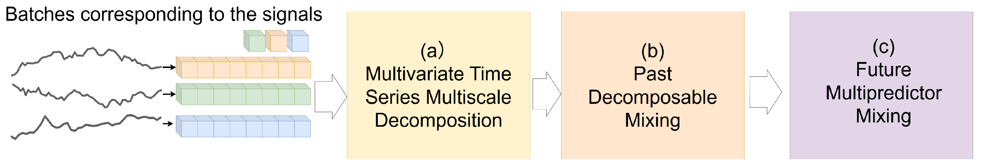
TimeMixer-FI(Feature Interaction) extends the original TimeMixer framework by incorporating the MLPMixer architecture to facilitate sophisticated feature interactions. Overview of the proposed framework as show in Figure 1. The process includes three main steps: (a) Multivariate Time Series Multiscale Decomposition, (b) Past Decompose Mixing, and (c) Future Multipredictor Mixing. On the left, batches corresponding to the signals are shown, with different colors representing distinct signals or channels. Arrows indicate the data flow through the three main steps, where step (a) decomposes the signals into multiscale components, step (b) mixes the decomposed components, and step (c) performs future prediction.
Unlike PCA [26], which produces independent principal components, UMAP’s dimensionality reduction preserves intricate topological relationships among features, resulting in a graph-like structure of interconnected components. Traditional linear layers are insufficient to capture these complex, nonlinear relationships between reduced dimensions.
The MLP-Mixer mechanism is introduced to facilitate comprehensive feature interaction learning through its dual-path mixing strategy. This enhancement enables the model to effectively capture both local and global feature dependencies, resulting in more nuanced representation learning. The combination of token-mixing and channel-mixing operations in MLPMixer provides an elegant solution for modeling the inherent graph-like relationships present in UMAP-reduced features, thereby improving the model’s ability to leverage the rich structural information preserved by UMAP transformation.

2.2.1. Multilayer Perceptron

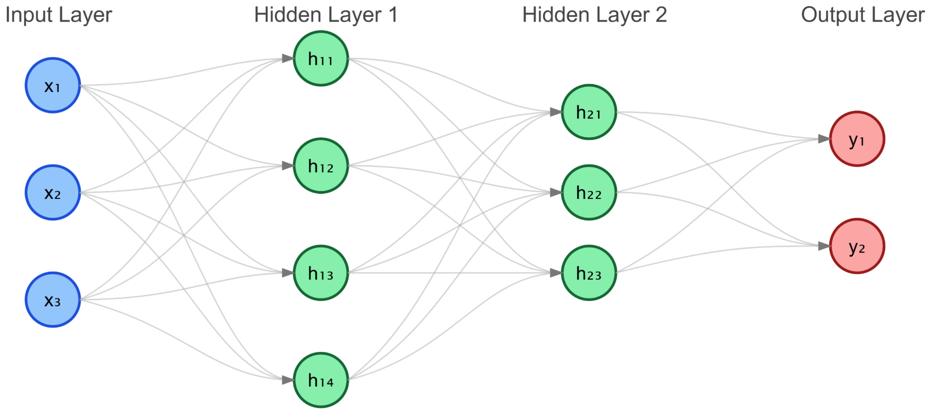
As a fundamental neural architecture, MLP enables effective handling of classification and regression tasks through its adaptive feedforward structure. This network comprises an input layer, multiple hidden layers, and an output layer, distinguished by its adaptability in modeling complex nonlinear relationships. The structural design is illustrated in Figure 2.
1. Architecture Design: The framework incorporates interconnected layers where information flows from input through hidden transformations to generate output predictions. Hidden layers utilize ReLU activation to introduce nonlinearity, defined by:
f ( x ) = max ( 0 , x )
2. Signal Propagation: Information traverses the network through sequential layer transformations. Each layer processes its input through linear operations followed by nonlinear activation:
h ( l ) = f W ( l ) h ( l 1 ) + b ( l )
where W ( l ) and b ( l ) denote the weight matrix and bias vector at layer l, h ( l 1 ) represents the previous layer output, and f indicates the activation function.
3. Optimization Framework: The network parameters are refined by minimizing objective functions—typically, MSE for regression or cross-entropy for classification tasks. Parameter updates utilize gradient computation through backpropagation, implementing optimization strategies like Adam [27] or SGD [28].
MLP’s effectiveness stems from its architectural simplicity combined with modeling versatility. The integration of hidden transformations and nonlinear activations enables capture of intricate data patterns, establishing MLP as a cornerstone component in deep learning applications. As shown in Figure 2, to disentangle complex variations, we first apply average pooling to the observation x R P × C , resulting in M low-dimensional sequences { x 0 , , x m } , where x m R P m × C and m { 0 , , M } . The lower-level sequence x 0 is the input sequence containing the finest scale variations, while the higher-level sequence captures more macro-level trends. We then embed these multi-scale sequences into a deeper feature representation z 0 = Embed ( X ) , which encodes the multi-scale properties of the sequence.
Next, we propose to decompose the past sequences and extract multi-scale historical information through a Progressive Decomposition Module (PDM) across layers. The output at layer l can be formalized as follows:
X l = PDM ( X l 1 ) , l { 0 , , L } ,
where L is the total number of layers, and X l = { x 0 l , , x M l } , where each sequence x m l R P m × C model represents a progressively refined representation of the input. The detailed operations of the PDM are described in the next section.
For the forecasting stage, we employ a Future Multiscale Mixer (FMM) module to aggregate the multi-scale information X L and generate the future prediction:
x ^ = FMM ( X L ) ,
where x ^ R F × C denotes the final predicted sequence. Through this design, the TiMixer architecture effectively captures essential past information and utilizes the strengths of multi-scale representations to forecast the future.

2.2.2. Construction of Multi-Scale Temporal Representations

To disentangle complex variations, the past observations x R P × C are first downsampled into M scales through average pooling, ultimately obtaining a set of multiscale time series x = x 0 , , x m , where x m R [ P 2 m ] × C , m { 0 , , M } , and C denotes the variate number. The lowest-level series x 0 = x represents the input series containing the finest temporal variations, while the highest-level series x M captures macroscopic variations. Subsequently, these multiscale series are projected into deep features X 0 through the embedding layer, which can be formalized as X 0 = Embed ( X ) 
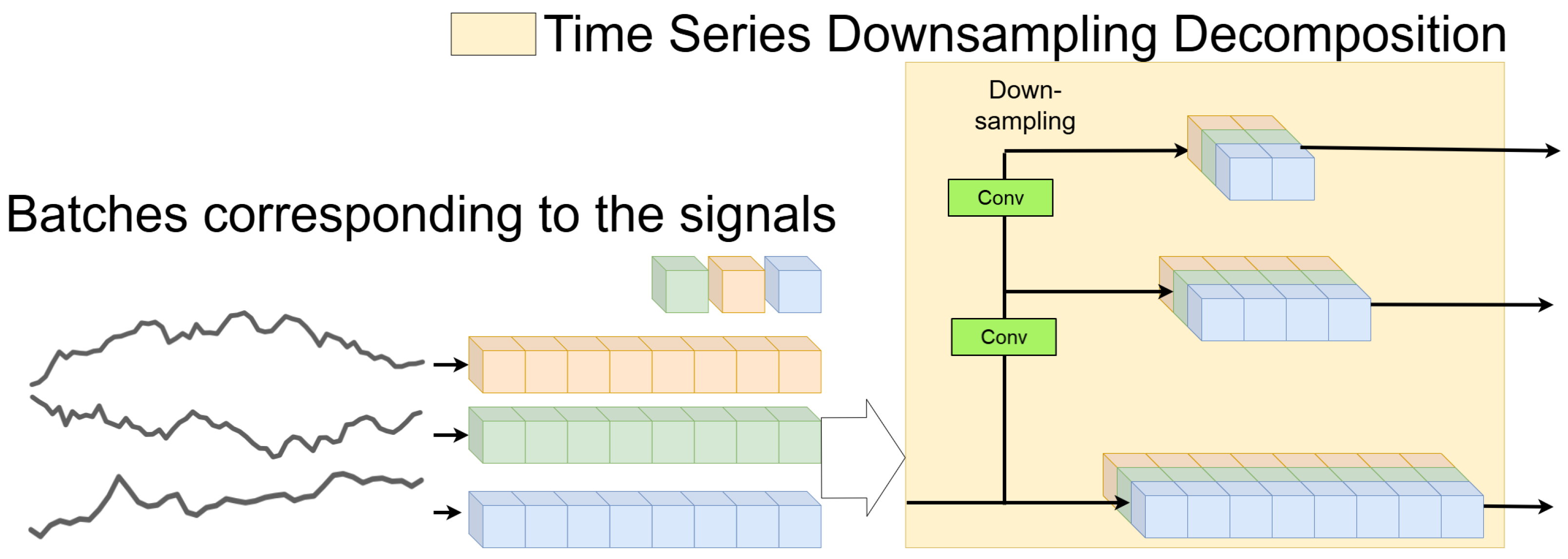
. Through the above designs, multiscale representations of the input series are obtained. Illustration of the Time Series Downsampling Decomposition process as show in Figure 3. The input signals (batches on the left) are processed through multiple Conv and Downsampling layers to decompose the time series into multiscale components. Different colors represent distinct signals or channels, with the output components at varying scales shown on the right. Arrows indicate the data flow through the Conv and Downsampling layers, where each layer reduces the temporal resolution to capture multiscale patterns.

2.2.3. Seasonal Component Mixing

In seasonal analysis, cyclical patterns can be detected over time, such as daily peaks in traffic volume. With time, sharp seasonal shifts occur, necessitating finer adjustments in future predictions. To this end, we employ a bottom-up approach to integrate the information across time scales, progressively refining the seasonal patterns from the coarse to finer scales.
For a set of seasonal components δ l = { δ 0 l , , δ M l } , we recursively compute the seasonal interaction at layer l as follows:
δ m l = δ m l + Bottom - Up - Mixing ( δ m 1 l ) + Feature Fusion ( δ m 1 l ) ,
where Bottom-Up-Mixing(·) is linear and operates across temporal dimensions using GELU activations, with input dimension P 2 m , and 
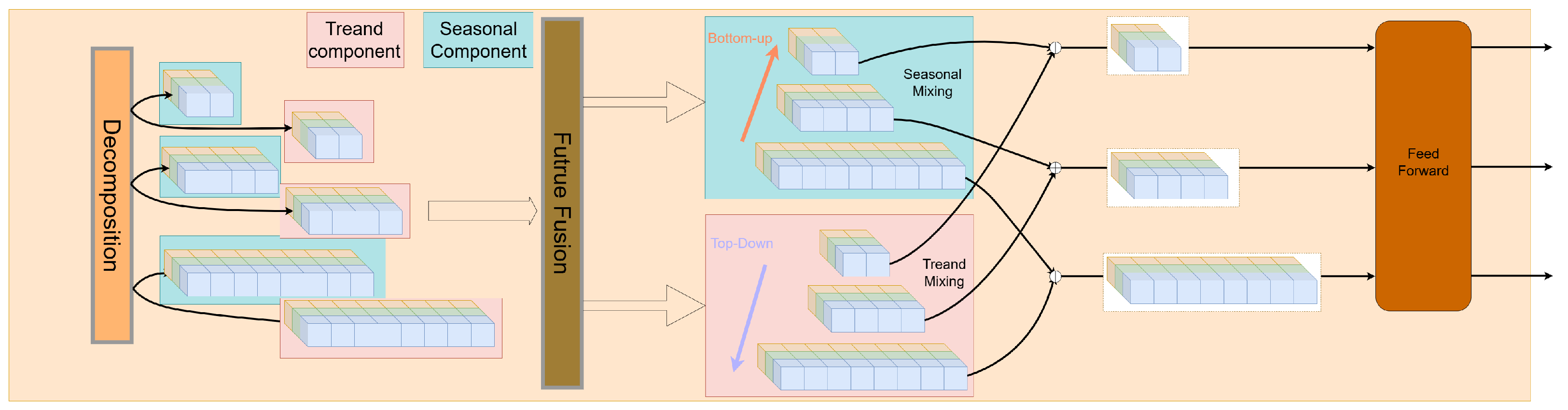
Feature Fusion(·) applies a LayerNorm followed by GELU. The structure of this module is shown in the Figure 4. Pink represents the trend component, blue represents the seasonal component, and orange indicates the decomposition process. The brown section on the right denotes the feed-forward process. Arrows (bottom-up in red and top-down in purple) denote the seasonal and trend mixing directions.

2.2.4. Trend Component Mixing

In contrast to the seasonal part, trend components often exhibit smoother, macro-level changes. Upper layers tend to contain coarse information, while lower layers reveal more refined variations. Thus, we apply a top-down mixing approach, using coarse scales to guide the refinement of the trend patterns across finer scales.
For a set of trend components τ m l = { τ 0 l , , τ M l } , we recursively compute the trend interaction as follows:
τ m l = τ m l + Top - Down - Mixing ( τ m + 1 l ) + Feature Fusion ( τ m + 1 l ) ,
where Top-Down-Mixing(·) uses GELU activations and progressively refines the trends with input dimension P 2 m .  Feature Fusion(·) is similar to the seasonal fusion process, involving two linear layers followed by GELU activations and LayerNorm.

2.2.5. Feature Fusion

Given input feature X i n , the Feature Fusion operation is defined as:
X o u t = T ( M L P ( L N ( C h ( P ( X i n ) ) ) ) + X i n
where P ( · ) denotes the patch operation, C h ( · ) represents the channel processing operation, L N ( · ) indicates Layer Normalization, and M L P ( · ) is the Multi-Layer Perceptron. T ( · ) represents the final transformation. For each channel i { 1 , 2 , 3 , 4 } , the operation can be formulated as follows:
Y i = M L P i ( L N ( X c ) )
where X c represents the channel-processed feature. Through this Feature Fusion module, we can effectively integrate multi-scale features while preserving the original information through skip connections. The structure of the Future Fusion module (highlighted in brown in Figure 4) as show in Figure 5. The module processes input data through LayerNorm, Patch, and multiple MLP layers with skip-connections. Different colors represent distinct channels of the input data, which are processed and fused across layers. The ‘T’ denotes a transpose operation to adjust the dimensions of the data, and arrows indicate the data flow with skip-connections enabling information transfer across layers.

2.2.6. Future Multiscale Forecasting Mixer

After processing through the PDM block, we acquire the multi-scale past information X L = { x 0 L , , x M L } , where x m L R P 2 m × d model . Since different scales of the sequence exhibit distinct primary variations, they also demonstrate different forecasting capabilities. To fully exploit this multi-scale information, we propose a future multiscale forecasting mixer (FMM), which generates predictions by combining predictions from various scales:
x ^ m = Predictor m ( x m L ) , m { 0 , , M } , x ^ = m = 0 M x ^ m ,
where x ^ m R F × C represents the future prediction at scale m, and the final output x ^ R F × C represents the predicted future sequence. Predictor m (·) refers to the predictor for the m-th scale sequence, which applies a linear layer to the final deepest feature representation from the previous layers, mapping it to the future sequence of length 
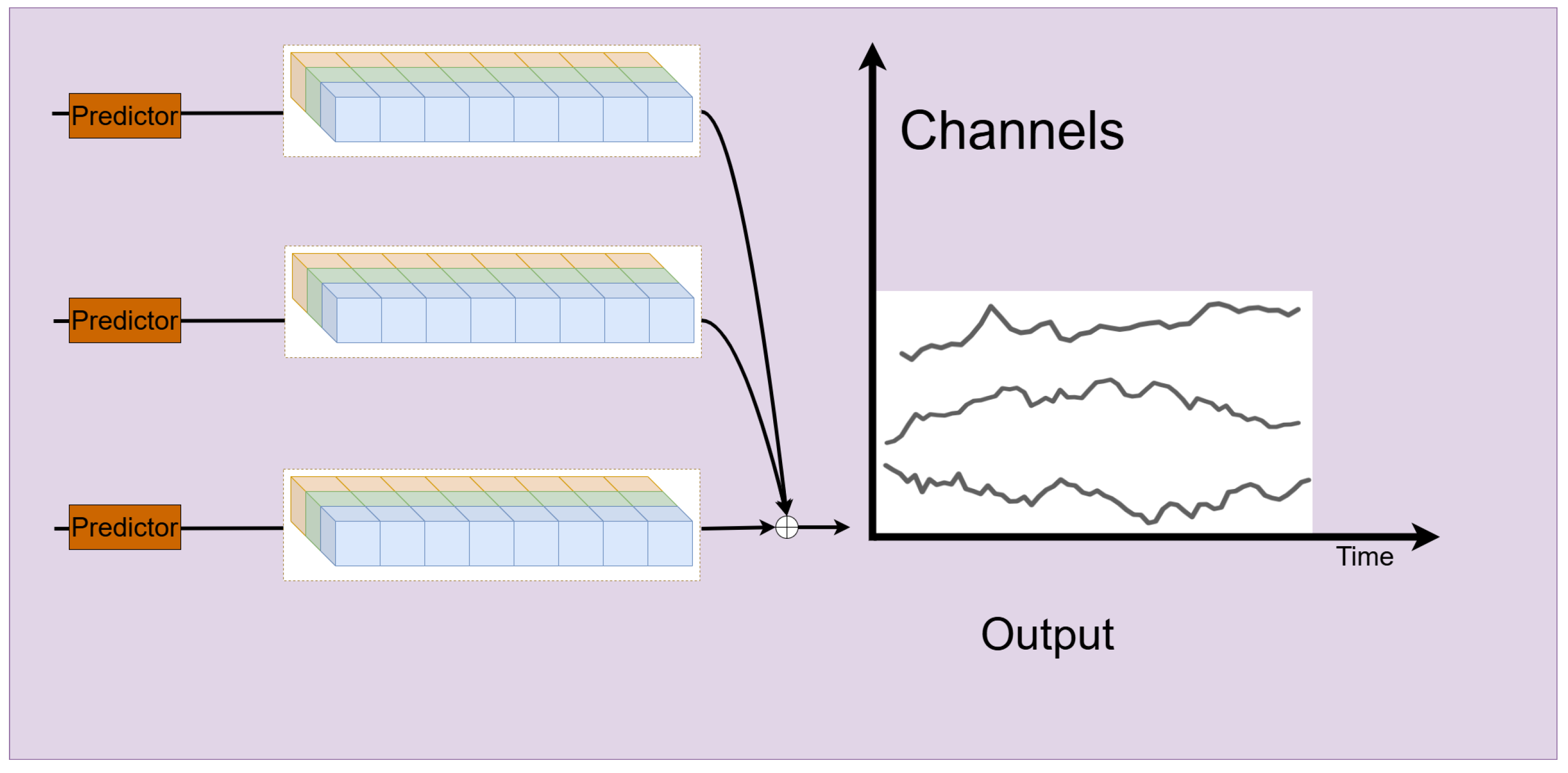
F. Notably, FMM aggregates multiple predictors, each utilizing the historical information from different scales. This aggregation enhances the predictive capabilities, especially in forecasting complex, multi-scale sequences. The structure of the Predictor module as show in Figure 6. The module processes multi-channel input data (represented by different colors) and generates the output time series. The vertical axis represents channels, and the horizontal axis represents time. Each predictor block processes a subset of channels to produce the final prediction. Arrows indicate the data flow from input to output through the Predictor blocks, and the output on the right shows the predicted time series for each channel.

3. Time Complexity Comparison: TimeMixer vs. TimeMixer-FI

To clearly demonstrate the similarity in computational complexity between the original TimeMixer and the modified TimeMixer-FI, we analyze their time complexities using big-O notation, parameterized by the batch size B, sequence length T, and number of channels C. Both models share highly consistent core modules, such as PastDecomposableMixing and MultiScaleMixing.

3.1. Itemized Complexity Breakdown

The time complexity decomposition for both models is as follows:
  • TimeMixer (Original Version)
    PastDecomposableMixing: O ( B · T · C · d ff ) , where d ff is the feedforward network dimension.
    MultiScaleSeasonMixing and MultiScaleTrendMixing: O ( B · C · T 2 ) , dominated by multi-scale downsampling/upsampling operations.
    Total Complexity: O ( B · C · T 2 ) .
  • TimeMixer-FI (Modified Version)
    PastDecomposableMixing: O ( B · T · C · ( d + d ff ) ) , with an added feature interaction term (d is the hidden dimension).
    MultiScaleSeasonMixing and MultiScaleTrendMixing: O ( B · C · T 2 ) , with additional interaction layers contributing O ( B · T · C · d ) .
    Total Complexity: O ( B · C · T 2 ) .

3.2. Key Comparison

The analysis reveals: Both models exhibit a total time complexity of O ( B · C · T 2 ) , primarily driven by multi-scale mixing operations.The additional computation introduced by TimeMixer-FI (e.g., feature interaction O ( B · T · C · d ) ) is a lower-order term, which becomes negligible compared to O ( B · C · T 2 ) when T is sufficiently large.
The following Table 1 provides a visual comparison of their complexities:

3.3. Conclusion

TimeMixer and TimeMixer-FI exhibit virtually identical time complexities, both totaling O ( B · C · T 2 ) . The additional computations in the modified version are limited to lower-order terms, rendering their impact negligible for large T. Thus, from both theoretical and practical perspectives, the computational costs of the two models are extremely similar.

4. Experiment

4.1. Data and Experiment Platform

The experiment utilizes operational data from the YUAN FU YANG, a 167,168 gross tonnage crude oil tanker operated by COSCO Shipping Energy Transportation and constructed by the Dalian Shipbuilding Industry Co., Ltd., Dalian, China. The data were collected using the marine equipment inspection manhole with an integrated temperature monitoring system (Figure 7), which measured exhaust gas temperatures across six cylinders and facilitated the recording of power output (Ps) during two operational phases: steady-state full-speed navigation and an abnormal rapid speed reduction event. These parameters were chosen for their strong internal relationships and correlation with engine performance, making them ideal for UMAP dimensionality reduction and fault detection analysis (Figure 8). The computational platform, equipped with an Intel Core i9-13900HX processor, an NVIDIA GeForce RTX 4090 Laptop GPU, CUDA 12.1, and PyCharm 2023.1.2 Professional Edition, was used for data preprocessing (denoising with Learnable Wavelet Packet Transform), UMAP dimensionality reduction, and training/evaluation of all models (Transformer, Autoformer, Informer, Dlinear, TimeMixer, and TimeMixer-FI). This setup ensured efficient processing of the high-dimensional data and enabled the experiments reported in Section 4.2 and Section 4.3.
Notably, UMAP exhibits stringent requirements for input data quality, with its performance heavily dependent on accurate local neighborhood structure construction. Since noise significantly interferes with distance metric accuracy and disrupts the authentic topological relationships between data points, preliminary signal denoising proves crucial for UMAP’s dimensionality reduction effectiveness. Moreover, given that UMAP relies on distance-based nearest neighbor computations, which can be skewed by features with differing scales, the engine data—comprising exhaust gas temperatures across six cylinders and power output (Ps)—was normalized prior to denoising. This normalization, scaling all features to a uniform range (e.g., [0, 1]), ensures that each feature contributes equally to the distance calculations, preventing features with larger magnitudes from disproportionately influencing the UMAP transformation, thus enhancing training stability and anomaly detection sensitivity. The experiment then employs the Learnable Wavelet Packet Transform (L-WPT) [29] for denoising, as it provides effective noise reduction while preserving essential signal characteristics. Due to UMAP’s focus on preserving topological structure rather than absolute magnitudes, no denormalization was performed post-processing, ensuring compatibility with its algorithmic requirements.
Figure 9 shows a comparison of the exhaust gas temperature signals from a six-cylinder engine, with the original signal above and the denoised signal below. The denoised signal is smoother, removes high-frequency noise, and retains the main features of the signal, which is conducive to subsequent fault diagnosis. Appropriate signal processing methods can effectively improve the quality of exhaust temperature signals and provide reliable data support for engine condition monitoring. Similarly, Figure 10 presents a comparison of the PS signal, with the original signal above and the denoised signal below.

4.2. UMAP Dimensionality Reduction and Feature Correlation Analysis

UMAP hyperparameters were empirically configured with default values: n_components = 2, n_neighbors = 15, and min_dist = 0.1. As a nonlinear dimensionality reduction technique, UMAP was employed to map high-dimensional engine operational data into a low-dimensional feature space, providing optimized input features for subsequent time series prediction models. To evaluate the sensitivity of UMAP’s performance to hyperparameter variations, we introduced the “local preservation rate” as a metric, defined as the percentage of k-nearest neighbors preserved after dimensionality reduction, i.e.,
Local Preservation Rate = 1 N i = 1 N | N N high ( i ) N N low ( i ) | k × 100 ,
where N is the number of data points, N N high ( i ) and N N low ( i ) are the sets of k-nearest neighbors for point i in the high-dimensional and low-dimensional spaces, respectively, and k is set equal to the n_neighbors parameter.
This metric quantifies UMAP’s ability to retain local structures, directly reflecting the impact of hyperparameters such as n_neighbors and min_dist. We conducted experiments with various hyperparameter combinations (e.g., n_neighbors ranging from 5 to 50 and min_dist from 0.1 to 0.9) on the marine diesel engine dataset, and the results demonstrated that the default parameters (n_components = 2, n_neighbors = 15, min_dist = 0.1) achieve the highest local preservation rate of approximately 55%, as illustrated in Figure 11 (refer to the blue line corresponding to min_dist = 0.1). These findings validate the effectiveness of the selected default hyperparameters in preserving local structures, thereby providing an optimal feature representation for fault detection in our study, while also indicating that UMAP’s performance is moderately sensitive to n_neighbors—with a 15% drop in local preservation rate as n_neighbors increases to 50—but relatively robust to changes in min_dist, with variations within 5%.
To evaluate the model’s behavior under real-world conditions with noisy data, we analyzed UMAP’s dimensionality reduction on raw, unprocessed signals (Figure 12). The resulting chaotic fluctuations suggest that without preprocessing, subtle fault signatures are obscured, reflecting challenges typical of noisy real-world scenarios. This is contrasted with the denoised results in Figure 13, where L-WPT preprocessing enhances pattern detection, demonstrating a practical workflow for real-world deployment. While this does not encompass all possible noise profiles, it provides an initial assessment of the model’s sensitivity to noise, with further real-world validation planned for future work.
The comprehensive analysis of feature relationships illustrated in Figure 13, Figure 14, Figure 15, Figure 16 and Figure 17 reveals significant nonlinear patterns and complex interdependencies that challenge traditional linear architectures. The feature interaction scatter plot (Figure 14) demonstrates intricate branching structures with curved trajectories and multiple bifurcations, while the feature space distribution (Figure 15) space distribution in two dimensions (Dim1 and Dim2). The density is visualized using a color gradient, where deep purple represents low-density regions, and bright green indicates high-density regions with local maxima. The distribution exhibits irregular density patterns with multiple local maxima, as evidenced by the non-uniform distribution of high-density regions. Dim1 and Dim2 are obtained through dimensionality reduction to visualize the high-dimensional feature space. The joint probability distribution (Figure 16) further corroborates this complexity through asymmetric coupling patterns, particularly visible in the irregularly distributed high-probability regions. Most notably, the local correlation analysis (Figure 17) exhibits dramatic fluctuations between [−1, 1], indicating strong context-dependent feature relationships that fundamentally violate the assumptions of linear transformations.
These observations conclusively demonstrate that simple linear layers are insufficient for capturing such sophisticated feature interactions. The presence of dynamic, context-dependent relationships, coupled with the non-uniform spatial distribution of feature dependencies, necessitates advanced architectural components, such as nonlinear activation functions, attention mechanisms, and residual connections, to effectively model these complex patterns. The empirical evidence establishes a clear requirement for sophisticated neural network architectures capable of modeling intricate feature relationships and nonlinear dependencies observed in the data distribution.
The empirical analysis indicates that conventional model architectures based on channel-independent processing or simple linear layers cannot adequately capture the complex feature interactions observed in temporal data. The integration of MLP-Mixer layers enhances the model’s capability to learn and utilize nonlinear feature dependencies, significantly improving predictive performance. This architectural enhancement enables more accurate capture of intrinsic data structures, establishing a robust feature representation foundation for state identification and prediction tasks. The improved architecture demonstrates superior capacity in modeling temporal dynamics and feature correlations, as evidenced by the comprehensive evaluation results. The enhanced feature interaction capabilities contribute to more reliable temporal pattern recognition and state transition modeling, addressing the limitations of traditional approaches in handling complex temporal dependencies.

4.3. Performance Evaluation and Early Warning Validation

To evaluate model performance systematically, an experimental framework was designed with fixed output length (60 time steps) and variable input lengths (60–600 time steps), aligning with practical ship engine monitoring requirements where fixed-horizon predictions utilize varying historical data lengths. The experimental results in Table 2 and Table 3 demonstrate the advantages of MLP-based architectures over attention-based approaches. The traditional attention-based models (Transformer, Autoformer, and Informer) showed significant performance deterioration with increasing sequence lengths. For instance, Transformer’s MSE increased from 0.1047 to 0.4598, while Autoformer and Informer exhibited even more substantial degradation, with MSE values rising to 0.6993 and 0.5599, respectively, at 600 time steps. This degradation highlights the limitations of attention mechanisms in processing extended sequences. In contrast, the pure MLP-based architecture of TimeMixer demonstrated superior stability, maintaining relatively consistent performance across different sequence lengths. The enhanced TimeMixer-FI model, incorporating additional MLP layers for feature interaction, further improved upon this foundation. At input length 60, TimeMixer-FI achieved an MSE of 0.0168 and MAE of 0.0549, significantly outperforming all baseline models. This performance advantage remained consistent across longer sequences—at 600 time steps, TimeMixer-FI maintained exceptional stability with MSE of 0.0198 and MAE of 0.0917, while other models showed substantial degradation. The comparison between TimeMixer and TimeMixer-FI particularly highlights the effectiveness of enhanced feature interaction modeling through additional MLP layers. TimeMixer-FI consistently achieved lower error rates across all sequence lengths, with MSE improvements ranging from 69.1% to 64.1% compared to the baseline TimeMixer. This consistent performance across varying temporal scales validates the effectiveness of strengthening feature interaction capabilities within the MLP architecture for complex time series prediction tasks.
Analysis of Figure 18 examines the model’s predictive performance during steady-state operation across three feature dimensions: The red line represents the predicted values of Feature 1 (Pred F1), the green line represents Feature 2 (Pred F2), and the blue line represents Feature 3 (Pred F3). The x-axis denotes time steps (0 to 40), and the y-axis represents the feature values.The detailed subplot analysis reveals nuanced performance patterns across features and batches during steady-state operation. Feature 1 (Power Output) demonstrates exceptional stability, with gradual upward trends in Batches 1–4 (MSE: 0.00–0.01) and near-perfect prediction in Batches 5–6. The first UMAP component (Feature 2) exhibits consistent downward trends, with steeper declines in early batches (MSE ≤ 0.00, MAE ≤ 0.02) and gentler slopes in later ones (MAE: 0.03–0.07). The second UMAP component (Feature 3) shows more varied behavior, transitioning from stable downward trends in Batches 1–2 to upward movements in Batches 3–4, and controlled oscillations in Batches 5–6, while maintaining acceptable error ranges. This hierarchical error distribution, where Feature 1 achieves the highest accuracy followed by Features 2 and 3, validates the model’s capability to capture both direct performance metrics and UMAP-reduced representations during steady-state operation.
As shown in Figure 19, the temporal prediction analysis during fault transition demonstrates distinct patterns across three features. The red line represents the predicted values of Feature 1 (Pred F1), the green line represents Feature 2 (Pred F2), and the blue line represents Feature 3 (Pred F3). For Feature 1 (power output), Batch 1 and Batch 2 show stable operation with minimal prediction errors (MSE: 0.01, MAE: 0.07 and MSE: 0.00, MAE: 0.01, respectively). The critical transition appears in Batch 3, where significant oscillations emerge (MSE: 0.00, MAE: 0.05), followed by pronounced deviations in Batch 4 (MSE: 0.17, MAE: 0.35). Batches 5 and 6 indicate system adaptation to the new operational state with sustained differences between the predicted and actual values (MSE: 0.03, MAE: 0.13 and MSE: 0.02, MAE: 0.12).
The UMAP-reduced dimensions (Features 2 and 3) demonstrate earlier detection of system anomalies compared to the raw power output (Ps). Specifically, Feature 2’s prediction divergence manifests significantly in Batch 2 with increasing error metrics (MSE: 0.03, MAE: 0.16), followed by Feature 3’s concordant deviation pattern in the same batch (MSE: 0.01, MAE: 0.19). In contrast, Ps maintains relatively stable predictions through Batch 3 with minimal errors (MSE: 0.00, MAE: 0.05), only showing substantial prediction deviations in Batch 4 (MSE: 0.17, MAE: 0.35). This sequential progression of error metrics across features—beginning with UMAP-reduced dimensions in Batch 2 and manifesting in power output during Batch 4—validates UMAP’s effectiveness in early anomaly detection through dimensional reduction.
Notably, after the system stabilizes in an altered operational state (Batches 5 and 6), a distinct difference emerges between UMAP-processed and raw data predictions. The raw power output (Ps) maintains relatively high prediction errors (MAE > 0.1), indicating sustained deviation from the original baseline. In contrast, the UMAP-reduced features demonstrate improved prediction accuracy during these batches, with errors returning to near-baseline levels (Feature 2: MSE: 0.00, MAE: 0.03; Feature 3: MSE: 0.00, MAE: 0.02). This phenomenon aligns with UMAP’s topological preservation principles as when the system settles into a new stable state, the data points form a new cluster in the reduced dimensional space, enabling accurate predictions despite the shift from initial operating conditions. While the UMAP-TimeMixer-FI framework effectively detects early faults using EGT-reduced features, it does not directly isolate individual cylinder contributions due to UMAP’s composite representation. Analysis of Figure 8’s EGT-Ps correlations suggests that cylinders with strong ties to Ps (e.g., Cylinder 1 or 6) are likely key contributors to anomalies, with early EGT deviations in Batch 2 (Figure 19) preceding Ps shifts. Engineers can pair model outputs with raw EGT logs to identify specific cylinder temperature changes driving these signals.

5. Conclusions

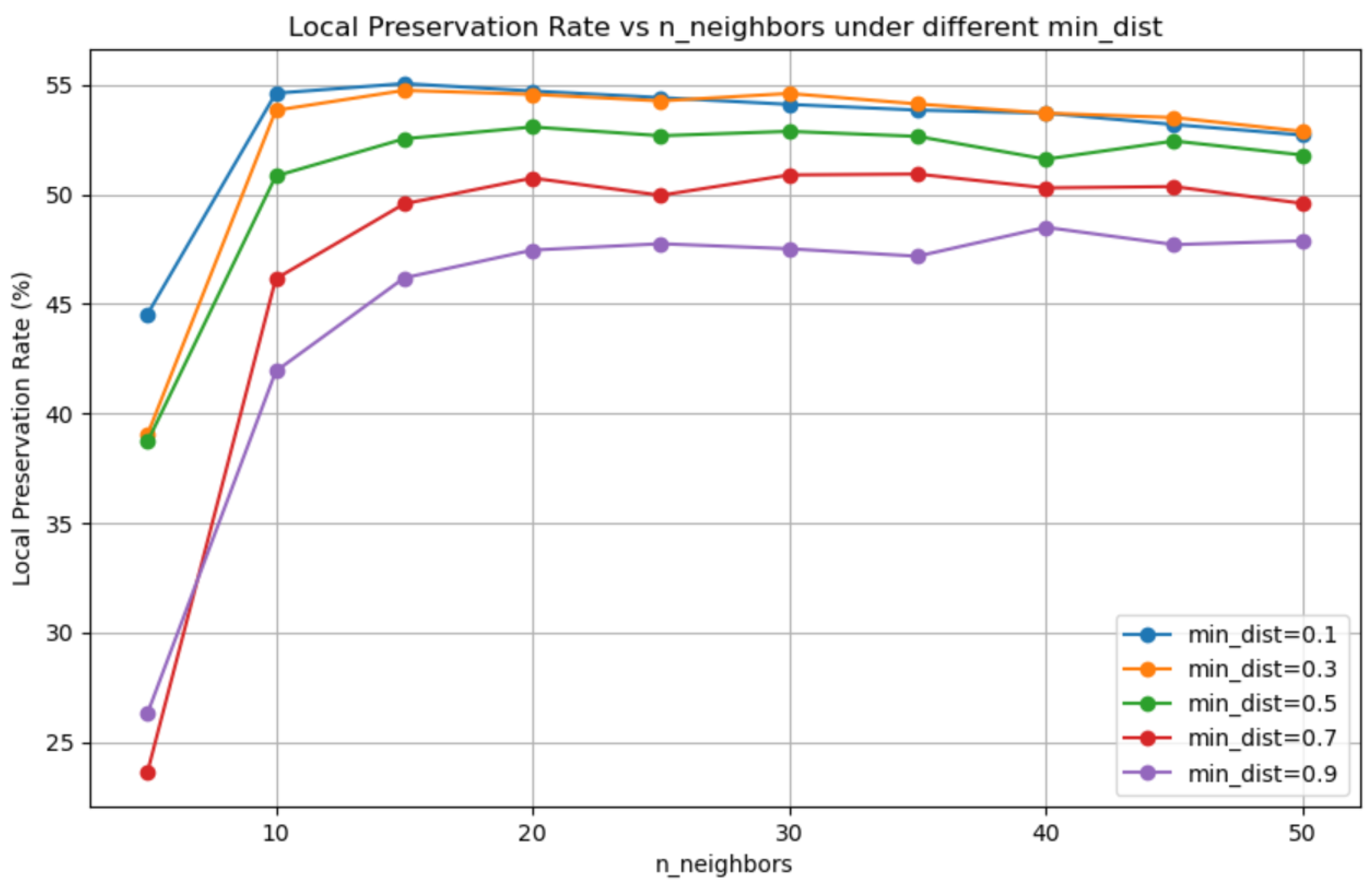
An unsupervised approach is introduced for early fault signals in marine diesel engines, combining UMAP dimensionality reduction with time series prediction to tackle the challenges of high-dimensional data and scarce fault labels in marine diesel engine fault diagnosis. UMAP effectively preserves topological structures and amplifies local differences, making subtle early fault signatures more detectable in the reduced dimensional space. To address the complex nonlinear relationships in UMAP-reduced features, the TimeMixer-FI model integrates MLP-Mixer layers, enhancing feature interaction modeling. The study concludes that this approach significantly improves fault detection, as validated by experiments: UMAP preserves topological structures with a local preservation rate of approximately 55% using default hyperparameters (Section 4.2, 
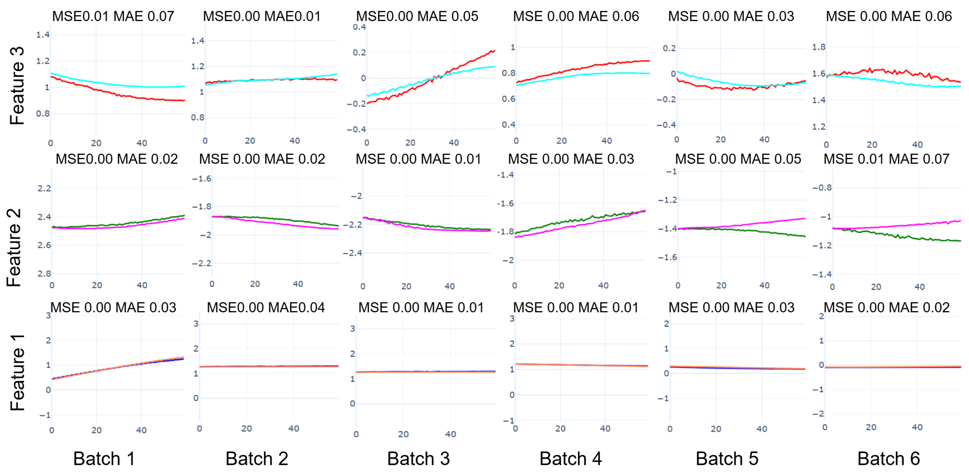
Figure 11), amplifying subtle anomalies, while TimeMixer-FI achieves a 69.1% MSE reduction (0.0544 to 0.0168) and 46.3% MAE reduction (0.1023 to 0.0549) at 60 time steps, enabling detection in Batch 2 (e.g., MSE 0.03, MAE 0.16 for Feature 2) versus Batch 4 for raw power output (MSE 0.17, MAE 0.35), two batches earlier, per Figure 16 (Section 4.3). Experiments demonstrate that TimeMixer-FI surpasses several baseline models in both steady-state and fault transition scenarios. By learning normal operating patterns as a baseline and monitoring deviations in the UMAP space, this approach detects anomalies before they significantly impact standard performance metrics, thereby improving the precision and efficiency of predictive maintenance in marine systems.
However, the current evaluation is limited to a single dataset from the YUAN FU YANG tanker, reflecting specific operational conditions (steady-state and rapid speed reduction), which may not fully represent diverse engine types or operating modes. Despite these advancements, practical deployment faces challenges, including: (1) model interpretability, as the complexity of UMAP and TimeMixer-FI may hinder engineers’ understanding of fault detection decisions; (2) generalization across diverse conditions, as varying marine environments or engine types may affect consistent fault detection; and (3) computational scalability, as the combined framework may demand substantial resources for real-time use on resource-limited shipboard systems. Future work will address these limitations by: (1) improving interpretability through feature importance analysis or UMAP embedding visualizations to clarify fault detection outcomes for engineers; (2) enhancing generalization with adaptive learning techniques to accommodate diverse marine conditions and engine variations, alongside testing on additional datasets; and (3) optimizing computational efficiency via model compression or lightweight architectures to ensure scalability for real-time shipboard applications. Future work could explore compatibility with optimization techniques like Bayesian Optimization to refine hyper-parameter tuning, enhancing model performance across diverse conditions.

Author Contributions

Methodology, S.D. and B.H.; formal analysis, S.D. and J.L.; writing—original draft preparation, S.D. and B.H.; writing—review and editing, B.H. and S.W.; visualization, M.Z.; supervision, B.H.; project administration, H.Z. and S.D.; funding acquisition, B.H. All authors have read and agreed to the published version of the manuscript.

Funding

This research received no external funding.

Data Availability Statement

We have published part of our research’s raw data at https://drive.google.com/file/d/1n6PYE5tCddKaj-R6LWB6DecTxtf-dyXd/view?usp=drive_link, accessed on 23 March 2025.

Conflicts of Interest

The authors declare no conflicts of interest.

References

  1. Toothman, M.; Braun, B.; Bury, S.J.; Moyne, J.; Tilbury, D.M.; Ye, Y.; Barton, K. Overcoming challenges associated with developing industrial prognostics and health management solutions. Sensors 2023, 23, 4009. [Google Scholar] [CrossRef] [PubMed]
  2. Lv, Y.; Guo, X.; Zhou, Q.; Qian, L.; Liu, J. Predictive maintenance decision-making for variable faults with non-equivalent costs of fault severities. Adv. Eng. Inform. 2023, 56, 102011. [Google Scholar]
  3. Qi, L.; Ren, Y.; Fang, Y.; Zhou, J. Two-view LSTM variational auto-encoder for fault detection and diagnosis in multivariable manufacturing processes. Neural Comput. Appl. 2023, 35, 22007–22026. [Google Scholar]
  4. Chen, Z.; O’Neill, Z.; Wen, J.; Pradhan, O.; Yang, T.; Lu, X.; Lin, G.; Miyata, S.; Lee, S.; Shen, C.; et al. A review of data-driven fault detection and diagnostics for building HVAC systems. Appl. Energy 2023, 339, 121030. [Google Scholar] [CrossRef]
  5. Wang, G.; Jin, S.; Zhao, G.; Zhao, J.; Xie, J. An independent component analysis based correlation coefficient method for internal short-circuit fault diagnosis of battery-powered intelligent transportation systems. Control Eng. Pract. 2023, 138, 105606. [Google Scholar]
  6. Huang, X.; Wen, Y.; Zhang, F.; Han, H.; Huang, Y.; Sui, Z. A review on risk assessment methods for maritime transport. Ocean Eng. 2023, 279, 114577. [Google Scholar]
  7. Singh, S.K.; Khawale, R.P.; Hazarika, S.; Bhatt, A.; Gainey, B.; Lawler, B.; Rai, R. Hybrid physics-infused 1D-CNN based deep learning framework for diesel engine fault diagnostics. Neural Comput. Appl. 2024, 36, 17511–17539. [Google Scholar]
  8. Woodyard, D. Pounder’s Marine Diesel Engines and Gas Turbines; Butterworth-Heinemann: Oxford, UK, 2009. [Google Scholar]
  9. Lv, Y.; Yang, X.; Li, Y.; Liu, J.; Li, S. Fault detection and diagnosis of marine diesel engines: A systematic review. Ocean Eng. 2024, 294, 116798. [Google Scholar]
  10. Orhan, M.; Celik, M. A literature review and future research agenda on fault detection and diagnosis studies in marine machinery systems. Proc. Inst. Mech. Eng. Part M J. Eng. Marit. Environ. 2024, 238, 3–21. [Google Scholar]
  11. Huang, M.; Liu, Z.; Tao, Y. Mechanical fault diagnosis and prediction in IoT based on multi-source sensing data fusion. Simul. Model. Pract. Theory 2020, 102, 101981. [Google Scholar]
  12. Li, X.; Cheng, C.; Peng, Z. Label-guided contrastive learning with weighted pseudo-labeling: A novel mechanical fault diagnosis method with insufficient annotated data. Reliab. Eng. Syst. Saf. 2025, 254, 110597. [Google Scholar] [CrossRef]
  13. Mejri, N.; Lopez-Fuentes, L.; Roy, K.; Chernakov, P.; Ghorbel, E.; Aouada, D. Unsupervised anomaly detection in time-series: An extensive evaluation and analysis of state-of-the-art methods. Expert Syst. Appl. 2024, 256, 124922. [Google Scholar] [CrossRef]
  14. McInnes, L.; Healy, J.; Melville, J. Umap: Uniform manifold approximation and projection for dimension reduction. arXiv 2018, arXiv:1802.03426. [Google Scholar]
  15. Demidova, L.A.; Stepanov, M.A. Approach to the analysis of the multidimensional time series based on the UMAP algorithm in the problems of the complex systems proactive maintenance. In Proceedings of the 2020 International Conference on Information Technologies (InfoTech), Varna, Bulgaria, 17–18 September 2020; IEEE: Piscataway, NJ, USA, 2020; pp. 1–4. [Google Scholar] [CrossRef]
  16. Altin, M.; Cakir, A. Exploring the Influence of Dimensionality Reduction on Anomaly Detection Performance in Multivariate Time Series. IEEE Access 2024, 12, 85783–85794. [Google Scholar] [CrossRef]
  17. Rezazadeh, N.; Polverino, A.; Perfetto, D.; De Luca, A. Dimensionality reduction in structural health monitoring: A case study on damaged wind turbine blades. In Macromolecular Symposia; Wiley: Hoboken, NJ, USA, 2024; Volume 413, p. 2400044. [Google Scholar] [CrossRef]
  18. Rezazadeh, N.; Annaz, F.; Jabbar, W.A.; Vieira Filho, J.; De Oliveira, M. A transfer learning approach for mitigating temperature effects on wind turbine blades damage diagnosis. Struct. Health Monit. 2025, 1–23. [Google Scholar] [CrossRef]
  19. Vaswani, A. Attention is all you need. In Advances in Neural Information Processing Systems; Neural Information Processing Systems Foundation, Inc.: Red Hook, NY, USA, 2017. [Google Scholar]
  20. Zhou, H.; Zhang, S.; Peng, J.; Zhang, S.; Li, J.; Xiong, H.; Zhang, W. Informer: Beyond efficient transformer for long sequence time-series forecasting. In Proceedings of the AAAI Conference on Artificial Intelligence, Virtual, 19–21 May 2021; Volume 35, pp. 11106–11115. [Google Scholar]
  21. Wu, H.; Xu, J.; Wang, J.; Long, M. Autoformer: Decomposition transformers with auto-correlation for long-term series forecasting. Adv. Neural Inf. Process. Syst. 2021, 34, 22419–22430. [Google Scholar]
  22. Si, C.; Yu, W.; Zhou, P.; Zhou, Y.; Wang, X.; Yan, S. Inception transformer. Adv. Neural Inf. Process. Syst. 2022, 35, 23495–23509. [Google Scholar]
  23. Zeng, A.; Chen, M.; Zhang, L.; Xu, Q. Are transformers effective for time series forecasting? In Proceedings of the AAAI Conference on Artificial Intelligence, Washington, DC, USA, 7–14 February 2023; AAAI Press: Palo Alto, CA, USA, 2023; Volume 37, pp. 11121–11128. [Google Scholar]
  24. Wang, S.; Wu, H.; Shi, X.; Hu, T.; Luo, H.; Ma, L.; Zhang, J.Y.; Zhou, J. Timemixer: Decomposable multiscale mixing for time series forecasting. arXiv 2024, arXiv:2405.14616. [Google Scholar]
  25. Peterson, L.E. K-nearest neighbor. Scholarpedia 2009, 4, 1883. [Google Scholar] [CrossRef]
  26. Abdi, H.; Williams, L.J. Principal component analysis. Wiley Interdiscip. Rev. Comput. Stat. 2010, 2, 433–459. [Google Scholar] [CrossRef]
  27. Zhang, Z. Improved adam optimizer for deep neural networks. In Proceedings of the 2018 IEEE/ACM 26th International Symposium on Quality of Service (IWQoS), Banff, AB, Canada, 4–6 June 2018; IEEE: Piscataway, NJ, USA, 2018; pp. 1–2. [Google Scholar]
  28. Keskar, N.S.; Socher, R. Improving generalization performance by switching from adam to sgd. arXiv 2017, arXiv:1712.07628. [Google Scholar]
  29. Frusque, G.; Fink, O. Robust time series denoising with learnable wavelet packet transform. Adv. Eng. Inform. 2024, 62, 102669. [Google Scholar]
Figure 1. TimeMixer-FI model flowchart.
Electronics 14 01293 g001
Figure 2. MLP structure.
Electronics 14 01293 g002
Figure 3. Details of multivariate time series multiscale decomposition (module (a) from Figure 1).
Electronics 14 01293 g003
Figure 4. Details of past decomposable mixing (module (b) from Figure 1).
Electronics 14 01293 g004
Figure 5. Details of feature fusion structure.
Electronics 14 01293 g005
Figure 6. Details of future multipredictor mixing (module (c) from Figure 1).
Electronics 14 01293 g006
Figure 7. Marine equipment inspection manhole with integrated temperature monitoring system.
Electronics 14 01293 g007
Figure 8. Multi-cylinder exhaust gas temperature (EGT) and Ps parameter correlation matrix.
Electronics 14 01293 g008
Figure 9. Comparison of exhaust gas temperature—Cylinder 1 signal denoising effects.
Electronics 14 01293 g009
Figure 10. Comparison of Ps signal denoising effects.
Electronics 14 01293 g010
Figure 11. Local preservation rate.
Electronics 14 01293 g011
Figure 12. UMAP visualization of raw signals without denoising.
Electronics 14 01293 g012
Figure 13. UMAP visualization of denoised signals.
Electronics 14 01293 g013
Figure 14. Feature interaction scatter.
Electronics 14 01293 g014
Figure 15. Feature space distribution.
Electronics 14 01293 g015
Figure 16. Joint probability distribution.
Electronics 14 01293 g016
Figure 17. Local correlation changes.
Electronics 14 01293 g017
Figure 18. Multi-feature temporal prediction analysis during steady-state operation.
Electronics 14 01293 g018
Figure 19. Multi-feature temporal prediction analysis during fault transition period.
Electronics 14 01293 g019
Table 1. Time Complexity Comparison of TimeMixer and TimeMixer-FI.
ModuleTimeMixerTimeMixer-FI
PastDecomposableMixing O ( B · T · C · d ff ) O ( B · T · C · ( d + d ff ) )
MultiScale Modules O ( B · C · T 2 ) O ( B · C · T 2 )
Total O ( B · C · T 2 ) O ( B · C · T 2 )
Table 2. Impact of input sequence length on model performance (MSE).
Model Name60120240480600
Transformer0.10470.14350.23920.42390.4598
Autoformer0.15040.23870.40040.59340.6993
Informer0.15350.20540.31180.49540.5599
Dlinear0.15880.17320.21060.20600.2160
PatchTST0.06230.11870.14760.09540.2539
TimeMixer0.05440.05520.04190.03730.0552
TimeMixer-FI0.01680.02050.02360.02440.0198
Table 3. Impact of input sequence length on model performance (MAE).
Model Name60120240480600
Transformer0.19360.23470.33150.47950.5137
Autoformer0.19770.27120.39920.54080.6109
Informer0.26480.30560.39930.52640.5749
Dlinear0.21330.23100.26860.28280.2958
PatchTST0.14520.12090.18030.15070.2451
TimeMixer0.10230.10460.09700.10220.1046
TimeMixer-FI0.05490.06720.06810.08070.0917
Disclaimer/Publisher’s Note: The statements, opinions and data contained in all publications are solely those of the individual author(s) and contributor(s) and not of MDPI and/or the editor(s). MDPI and/or the editor(s) disclaim responsibility for any injury to people or property resulting from any ideas, methods, instructions or products referred to in the content.

