Abstract
Orthogonal time frequency space (OTFS) modulation is a promising waveform for future wireless communication, offering robustness against time-varying channels and Doppler effects in high-mobility scenarios. However, the anti-jamming capabilities of OTFS systems remain underexplored, leaving gaps in understanding their potential in jamming-prone environments. In this work, we mainly focus on the jamming detection and suppression methods for OTFS systems in additive an white Gaussian noise (AWGN) channel. A frequency-domain anti-jamming technique is presented, employing a time-domain overlapping window approach to reduce jamming sidelobes while mitigating the signal-to-noise ratio (SNR) degradation caused by the window function. Additionally, a smoothing window method is introduced to provide stable samples for jamming detection, effectively reducing the false alarm rate. Furthermore, a low-complexity improved forward consecutive mean excision (FCME) algorithm is proposed, enhancing its practicality and making it more suitable for real-world applications. Finally, the effectiveness of the proposed anti-jamming methods is validated through simulation analyses under single-tone and partial-band jamming scenarios.
1. Introduction
The sixth-generation (6G) network is envisioned as a groundbreaking technology that enables seamless terminal applications across terrestrial and non-terrestrial domains, such as self-driving autonomous cars, high-speed trains, unmanned autonomous vehicles (UAVs), and low-earth-orbit (LEO) satellites [1,2,3]. Future 6G networks are anticipated to handle mobility speeds of up to 1000 km/h, representing a significant advancement over the capabilities of previous generations [4,5]. A key challenge in these scenarios is ensuring reliable communication in environments characterized by high mobility.
Orthogonal time frequency space (OTFS) is a novel two-dimensional (2D) modulation technique that offers superior resilience to Doppler and delay effects compared to conventional orthogonal frequency division multiplexing (OFDM) [6,7]. In recent years, a variety of studies have been conducted on the application of OTFS in different scenarios. In [8], the authors proved that the OTFS modulation is robust to carrier frequency offsets and performs better than OFDM modulation in LEO satellite communications. The Doppler interference in OTFS-based LEO satellite systems is analyzed in [9], and a simple yet practical solution to mitigate this interference is subsequently proposed. Furthermore, the authors in [10] proposed a multiple input multiple output (MIMO)-OTFS-based random access method for cooperative LEO satellite networks. Since 6G systems will adopt integrated space–air–ground–sea communications to achieve ubiquitous connectivity, anti-Doppler modulation and demodulation schemes, including OTFS and second-order time–frequency (SOTF) modulation, for high-mobility satellite–UAV communications were studied in [11,12,13]. Similar to OFDM, OTFS systems are also vulnerable to jammings [14]. Therefore, how to mitigate the impact of jamming in these communication systems has become a challenge.
There have already been several studies on the anti-jamming capabilities of OTFS. In [15], the authors explored narrow-band interference (NBI) in OTFS systems, emphasizing that OTFS demonstrates a certain level of robustness against NBI. In [16], an energy concentration NBI suppression method was proposed by designing the translation matrices and interference nulling. To address Barrage Jamming (BJ) in electromagnetic battlefield environments, the authors in [17] designed an OTFS with an Index Modulation (OTFS-IM) system and analyzed the impact of BJ on its performance. In [18,19], sparse code multiple access (SCMA) and a frequency hopping mechanism were proposed for NBI in the next generation of the Internet of Things (IoT). The non-uniform impact of jamming signals, such as NBI and periodic impulse noise (PIN), on OTFS systems was investigated, and a resource hopping method for OTFS-SCMA was developed to suppress severe interference [20]. In addition, researchers have proposed a variety of algorithms to address the problem of jamming detection [21]. Several notable approaches have been introduced, such as consecutive mean excision (CME) [22], forward consecutive mean excision (FCME) [23,24], FCME with double-threshold enhancement [25], and FCME incorporating adjacent cluster combining (ACC) techniques [26,27]. The CME algorithm operates under the assumption that the original received signal is jamming-free and iteratively compares signal amplitudes against an updated threshold to identify the jamming.The FCME algorithm assumes low-amplitude signals are jamming-free and uses lower detection thresholds to avoid missing low-power interference. However, its sorting process adds complexity, hindering hardware implementation. In summary, research on low-complexity jamming detection and suppression methods for OTFS remains limited.
In this work, a frequency-domain anti-jamming technique was explored, utilizing a time-domain overlapping window strategy to reduce interference sidelobes while mitigating the degradation of the signal-to-noise ratio (SNR) caused by the window function. A smoothing window technique was also employed to provide stable samples for interference detection, effectively reducing the false alarm rate. Finally, a low-complexity improved FCME algorithm was proposed.
The remainder of this paper is organized as follows. In Section 2, the system model is introduced. Section 3 shows the improved FCME algorithm based on overlap windowing for jamming detection. Section 4 shows that the proposed jamming detection and jamming suppression has better performance against single-tone and partial-band jamming than conventional ones through simulations. Section 5 draws the conclusions.
2. System Model
2.1. OTFS System
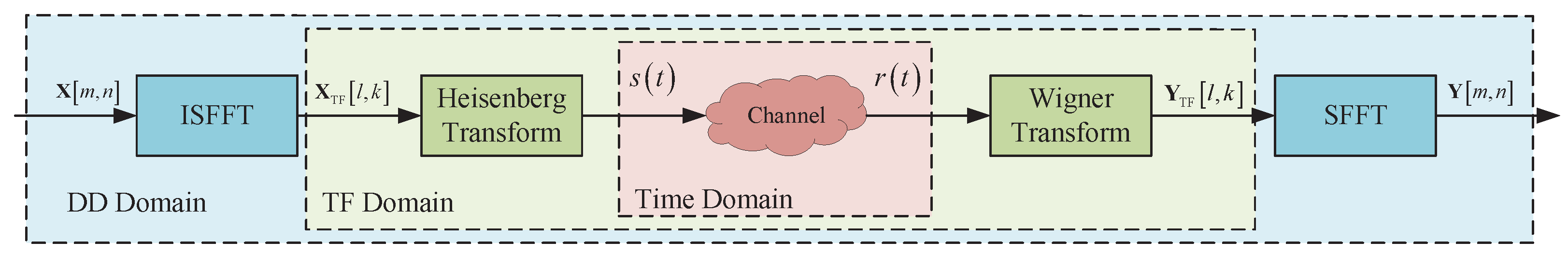
The diagram of the OTFS system is illustrated in Figure 1. At the transmitter end, the modulated information symbols are placed in the delay-Doppler domain grid , where M, N, , and T denote the delay dimension, Doppler dimension, subcarrier spacing, and time sampling interval, respectively.
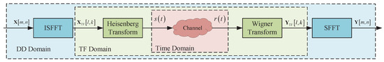
Figure 1.
Diagram of the OTFS system.
Using an inverse symplectic finite Fourier transform (ISFFT), the symbols are mapped to samples in the time–frequency domain as
where and . The ISFFT refers to 2D transformation, where each column of undergoes an M-point FFT, followed by an N-point IFFT on each row. Next, a Heisenberg transform is employed to convert the time–frequency signal to a continuous time-domain signal as
where is the transmit shaping filter. Considering an AWGN channel, the received signal can be expressed as , where denotes the noise component.
At the receiver end, the received signal is first match-filtered using a receive shaping filter as follows:
Sampling on forms the time–frequency domain received samples matrix as
for and . These two steps are collectively known as the Wigner transform, which samples the received signal and organizes it into a matrix. Finally, a symplectic fast Fourier transform (SFFT) is applied on to recover the original modulated information symbols as
2.2. Jamming Model
The single-tone jamming signal refers to a sinusoid signal as , in which , , and are the power, carrier frequency, and initial phase of the jamming signal, respectively. The single-tone jamming signal after sampling can be given by
where m denotes the index of the nearest subcarrier to the jamming signal’s center frequency, and represents the relative frequency offset of the jamming signal from the nearest subcarrier. We can also obtain the frequency-domain representation of the single-tone interference through N-point FFT as follows:
We can conclude that when the normalized frequency aligns perfectly with an integer multiple of the subcarrier spacing (i.e., ), the single-tone jamming primarily affects the corresponding subcarrier, leaving others unaffected. However, when , spectral leakage occurs, causing the jamming to spread across multiple subcarriers and significantly degrading system performance.
Another very important type of jamming is the partial-band jamming. This type of jamming is particularly effective in scenarios where attackers aim to disrupt communication across a broader portion of the frequency spectrum while conserving power. Partial-band jamming refers to jamming signals whose power is concentrated within a specific portion of the useful signal bandwidth. The jamming factor is defined as , where and B represent the bandwidth of the jamming signal and transmitted signal, respectively. Specifically, indicates the absence of jamming, represents full-band jamming, and denotes partial-band jamming.
For simplicity, the partial-band jamming signal is modeled as white Gaussian noise filtered by a band-limiting filter with a center frequency . The frequency response function of the filter can be expressed as
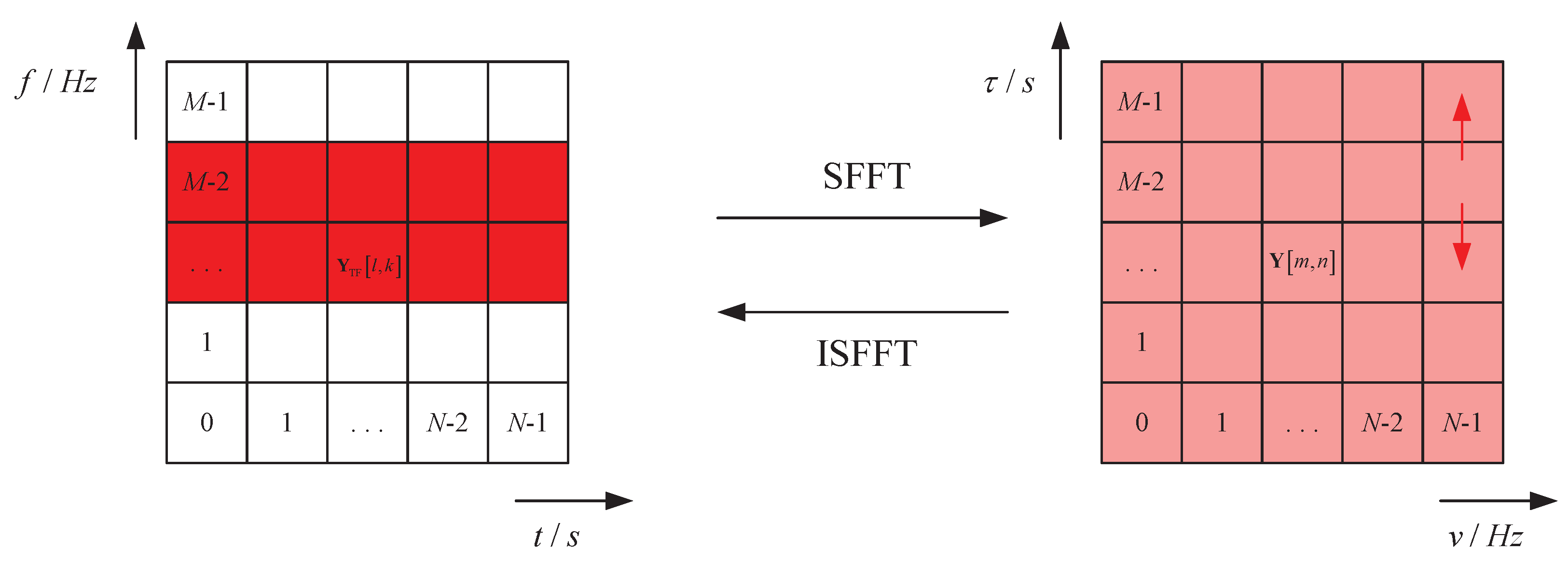
The common characteristic of single-tone and partial-band jamming is that the energy of the jamming signal is concentrated at one or more specific frequency points. As shown in Figure 2, the jamming signal spreads in the DD domain when transformed using SFFT. Therefore, it is more effective for us to detect and suppress the corresponding jamming signals in the time–frequency domain.

Figure 2.
Partial-band jamming in time–frequency domain and delay-Doppler domain.
2.3. Jamming Suppression Technique
Once the jamming signals have been recognized and the detailed frequencies are obtained, jamming suppression techniques can be employed to mitigate the adverse impact of interference. The most commonly used methods are nulling suppression and clipping suppression.
Let denotes the FFT result of received signal and represent the frequency index set of the jamming signal. The nulling suppression method can be expressed as
Signals identified as jamming are completely eliminated by setting their values to zero. This approach can effectively remove strong interference; however, it may also result in the loss of some useful signals, particularly when the interference overlaps with the signal spectrum.
The clipping suppression method mitigates the jamming signal by limit the amplitude of the signal to a certain threshold, which can be expressed as
where presents the mean value of for all k, and is the clipping factor. With this technique, the phase information is retained; however, residual interference may remain if is not appropriately chosen, which can affect subsequent demodulation performance.
3. Jamming Detection and Suppression in the Frequency Domain
In an AWGN channel, the received signal can be expressed as , where represents the noise component with zero mean and variance . To mitigate the adverse effects caused by jamming signals, we must first detect the presence of jamming and then suppress it using appropriate methods. In this section, details of jamming detection using the improved FCME algorithm and jamming suppression techniques are sequentially presented.
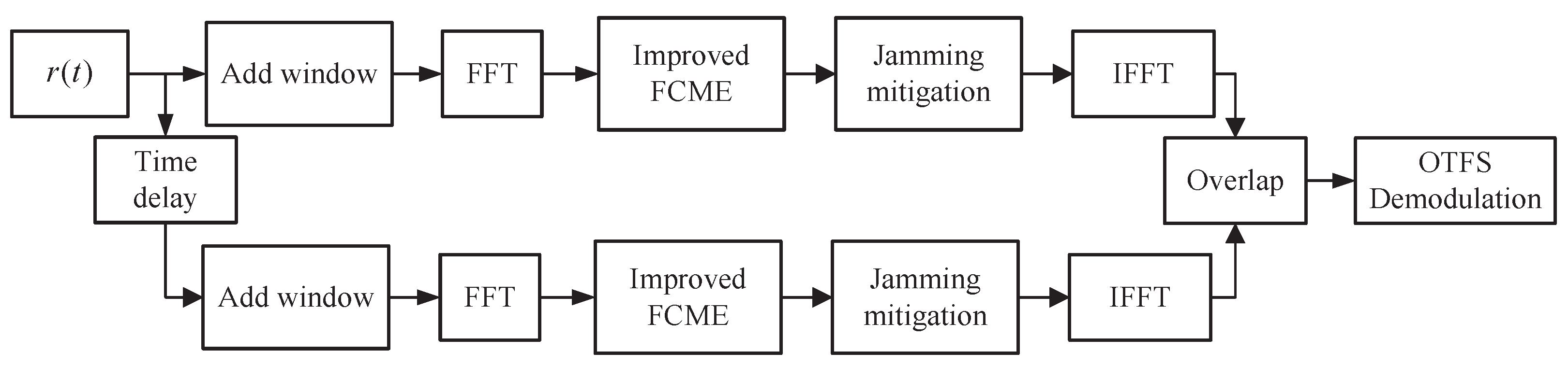
The overall block diagram of the anti-jamming OTFS receiver is illustrated in Figure 3. Since the FFT is applied to finite-length data segments, the resulting frequency spectrum is inherently discrete and limited in resolution. This limitation must be addressed when designing frequency-domain anti-jamming techniques to ensure accurate jamming detection and suppression. To mitigate spectral leakage effects, an overlapping window filter approach is introduced prior to the FFT operation. Then, the jamming signals are detected and suppressed after the FFT. Finally, the overlap-add method is applied to reconstruct the original signal for OTFS demodulation. In the following part of this section, we discuss the implementation details and parameter selection in detail.
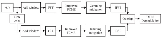
Figure 3.
Partial-band jamming in time–frequency domain and delay-Doppler domain.
3.1. Overlapping and Windowing
In the anti-jamming OTFS receiver, the received signal is divided into two consecutive overlapping frames and multiplied by a smoothing window to reduce amplitude discontinuities at their boundaries. The selection of the window function is a critical factor that demands thorough consideration. The Hamming window, Hanning window, and Blackman window are commonly used window functions that help suppress spectral leakage and improve frequency response performance. Since the received signal may suffer distortion after being filtered by the window function, SNR degradation can occur, negatively impacting BER performance. In this subsection, we evaluate the SNR loss caused by the windowing process and use it as a criterion for selecting the most appropriate window function.
The filtered signal in the frequency domain can be expressed as
where is the window function and the symbol ∗ denotes the convolution operator. The SNR gain caused by windowing the signal can be expressed as
where T is the sampling interval and is the length of window function. Table 1 presents the SNR gain caused by different window functions, where a negative gain indicates that the windowing process leads to SNR degradation. Additionally, the Hamming window function results in the least SNR degradation.

Table 1.
SNR gain caused by different window functions.
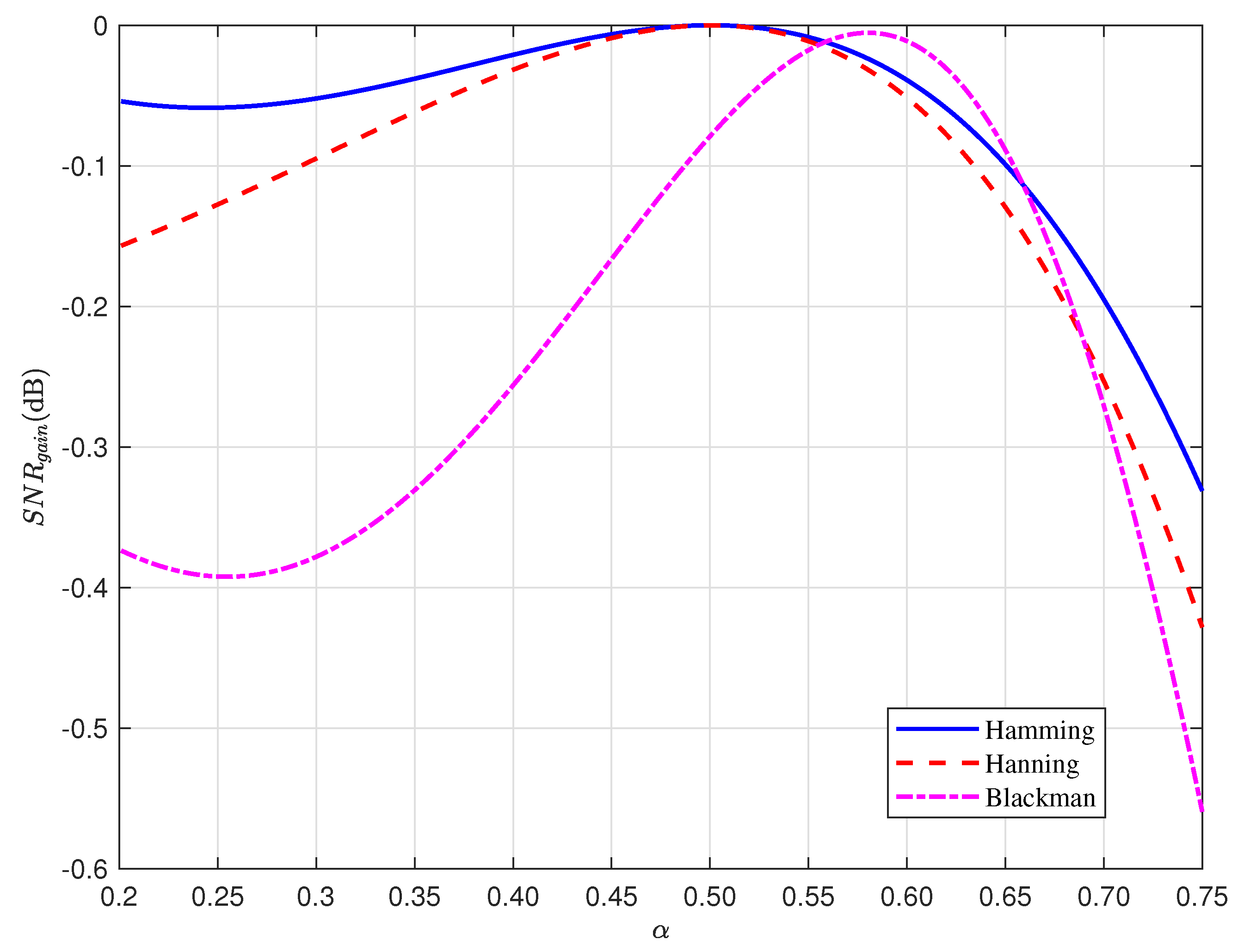
In order to compensate the SNR loss caused by the window filtering, an overlap window technique is introduced. The overlap ratio parameter must be carefully selected to achieve a better trade-off between SNR loss and computational cost. The relationship between the overlap ratio and the SNR gain achieved by adding an overlap window can be expressed as
Figure 4 illustrates the relationship between the overlap ratio and the SNR gain achieved by applying an overlap window with different window functions, including the Hamming, Hanning, and Blackman windows. It can be observed that the overlapping windowing technique effectively mitigates SNR degradation. However, this technique comes at the cost of increased computational complexity, which grows proportionally with the overlap ratio. Simulation results also show that the Hamming window function experiences less SNR degradation compared to the Hanning and Blackman window functions over a wide range of overlap ratios. Additionally, the minimum SNR degradation occurs when . As a result, the Hamming window function is employed, and the overlap ratio is set to 0.5 for the subsequent analysis.
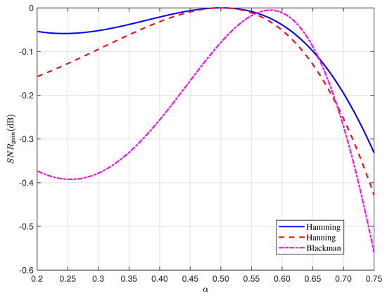
Figure 4.
The relationship between the overlap ratio and the SNR gain achieved by adding an overlap window using different window functions.
3.2. Smoothing Window Process
In OTFS systems, jamming detection can be significantly impacted by abrupt variations in signal power. To mitigate this, smoothing window processing is applied to stabilize the spectral characteristics of the received signal, ensuring a more uniform sample for jamming detection. By suppressing power fluctuations, this method reduces the probability of false alarms in interference detection and improves the accuracy of subsequent signal processing.
The smoothing window is applied in the frequency domain, averaging the power spectrum over a defined range. Specifically, for the frequency point k, the amplitude of the signal at this point is denoted as . The smoothing window processing involves selecting D frequency points on both sides of the target frequency point k. For a total of frequency points , their amplitudes are averaged to obtain . This value, , is then used as the smoothed amplitude of frequency point k. When or , meaning that fewer than D frequency points are available on either side of p, all available points are included in the averaging. The calculation is defined as
According to Equation (14), the smoothing window operation is defined as the weighted average of the magnitudes of all points within the window. Specifically, the first term on the right-hand side represents the case where the frequency point is within the first D positions, in which case the smoothing window remains fixed over the first D points without sliding. The second term corresponds to the case where the frequency point is within the last D positions, meaning the smoothing window remains fixed over the last D points without sliding. The third term describes the scenario where the frequency point is in an intermediate position, outside of the aforementioned two cases, which the smoothing window slides with the current frequency point as its center.
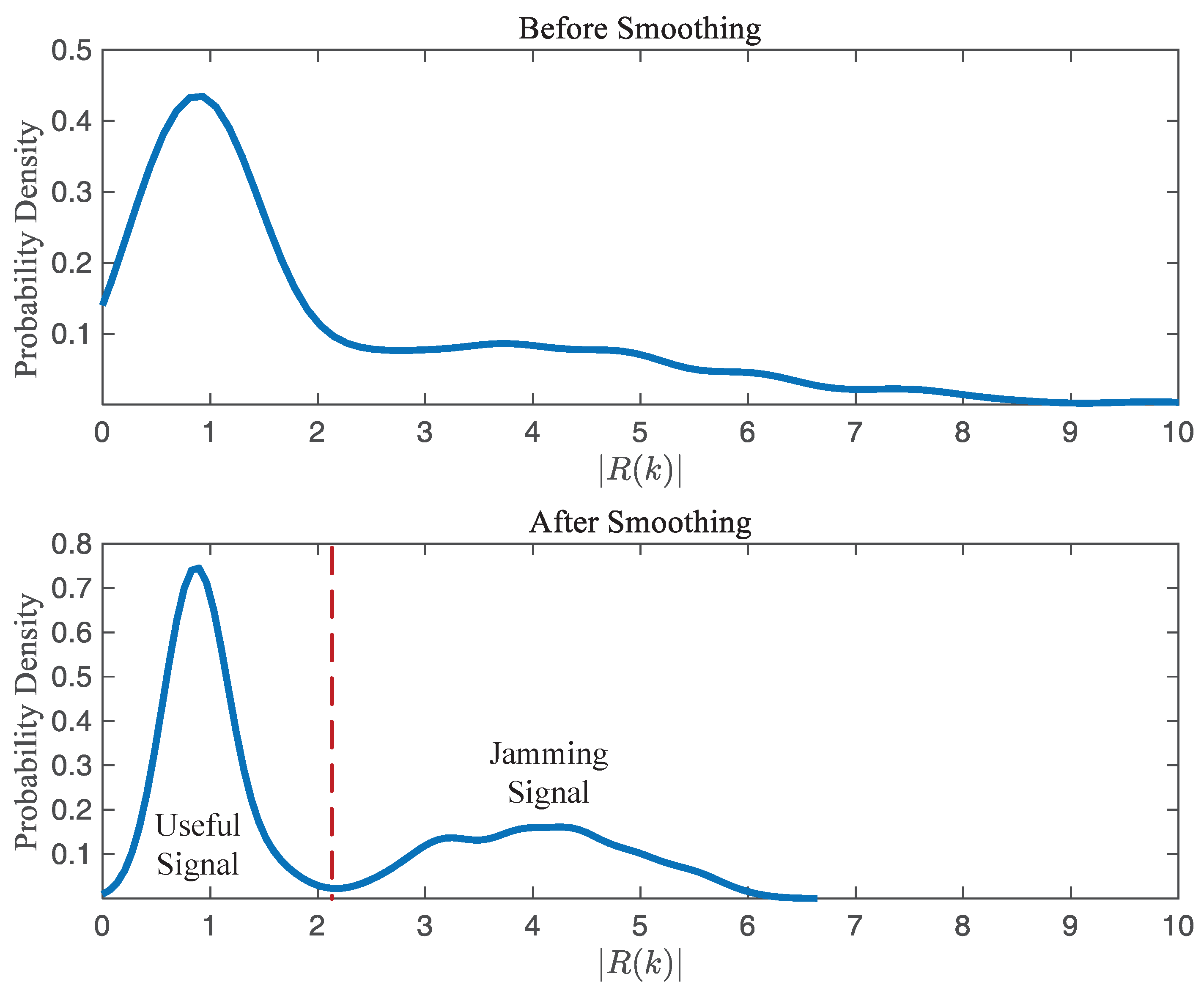
Here, the length of D is defined by the smoothing factor , where , and denotes the smallest integer value greater than or equal to . The smoothing factor represents the proportion of frequency points considered for weighted averaging within each smoothing window. Since the primary objective of smoothing is to mitigate high-power false alarms caused by non-jamming signals, the smoothing factor should be regarded as a trade-off between detection performance and false alarm probability. Figure 5 illustrates the probability density of the frequency-domain amplitudes of the received signal before and after smoothing. It is clearly observed that after processing with the smoothing window, a distinct boundary is formed between the amplitudes of the useful signal and the interference. This provides a stronger foundation for the detection process, facilitating more accurate differentiation between useful signals and interference, thereby improving the accuracy of jamming detection.
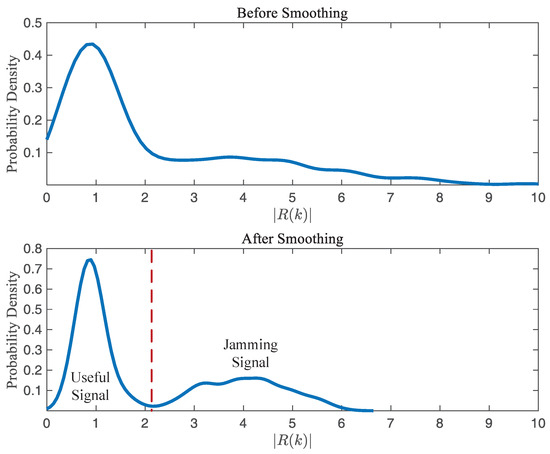
Figure 5.
The probability density of with and without smoothing window.
3.3. Improved FCME Algorithm
The CME and its variants, including the FCME, double-threshold-based FCME, and adjacent cluster combing (ACC)-based FCME, are widely used methods for jamming detection. The core idea of these algorithms are to iteratively identify and exclude frequency bins with energy levels greater than a given threshold, recalculating the mean of the remaining data points at each step to refine the threshold.
The primary difference between the CME and FCME algorithms lies in their initialization phases. The FCME algorithm assumes that low-amplitude signals are free of jamming, whereas the CME algorithm initially considers all signals to be free of jamming. The FCME algorithms begin with a lower initial threshold, increasing their likelihood of detecting jamming in scenarios with low jamming power. Despite their superior jamming detection performance, FCME-based algorithms require a sorting operation in the very beginning, which may result in high computational complexity. Generally, we need to find the smallest 10% of the frequency samples. The complexity of sorting depends on the sorting method. For example, Heapsort has a complexity of [28].
In this work, we propose an improved FCME algorithm that reduces sorting complexity while maintaining detection performance.
The flow chart of the proposed algorithm is as shown in Figure 6. Different from the conventional FCME algorithm, we did not need to perform complex sorting of frequency amplitudes to evaluate the power of the useful signal and determine the interference threshold. Instead, we divide the received signal frequency into Z segments with length as
and . Hence, we can evaluate the mean absolute value of each as
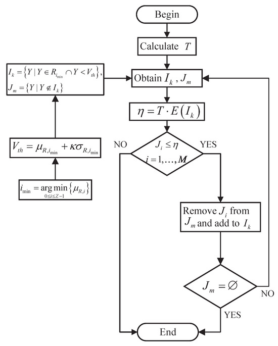
Figure 6.
The flow chart of proposed FCME algorithm.
Furthermore, we can find the segment with the minimum as
As shown in Equation (17), a total of comparisons are required to determine the position of the minimum value , which certainly possesses lower computational complexity than the traditional FCME method. Consequently, the mean absolute value and variance of the th segment can be used for the initial threshold calculation as
where and represent the mean absolute value and variance of the th signal segment, respectively. represents the weighting factor for the standard deviation in the preliminary decision threshold within each segment. It influences the number of samples used for local initialization to a certain extent. Although this method also involves comparison operations, it only requires finding the minimum value, and the dataset used for comparison is significantly reduced. As a result, the computational complexity is greatly decreased. In the subsequent steps for jamming detection, the operations are the same as those in the conventional FCME algorithms. Furthermore, the detection performance of our proposed FCME algorithm is evaluated in the next section.
The proposed FCME method was designed and implemented on a Xilinx Kintex XC7K325T FPGA. Table 2 summarizes the implementation results of the proposed method and the traditional FCME method. Our implementation consumes fewer look-up tables (LUTs), flip-flops (FFs), and Block RAMs (BRAMs) than the traditional method, demonstrating its low implementation complexity.
Table 2.
FPGA implementation results of different FCME methods.
4. Simulation Results
In this section, the performance of jamming detection and suppression is verified through simulations. We consider an uncoded OTFS system with , , and QPSK modulation.
4.1. Jamming Detection Performance
In this work, jamming detection performance is evaluated using the detection probability and false alarm probability . Here, is defined as the ratio of the number of successfully detected jamming frequency points to the total number of actual jamming frequency points. represents the ratio of falsely identified interfered frequency points to the total number of frequency points that are not interfered. In simulations, the SNR is set to 8 dB, and the segment number Z is set to 16 for the improved FCME algorithm. Finally, the detection performance of the proposed algorithm is compared with that of the CME algorithm and the FCME algorithm.
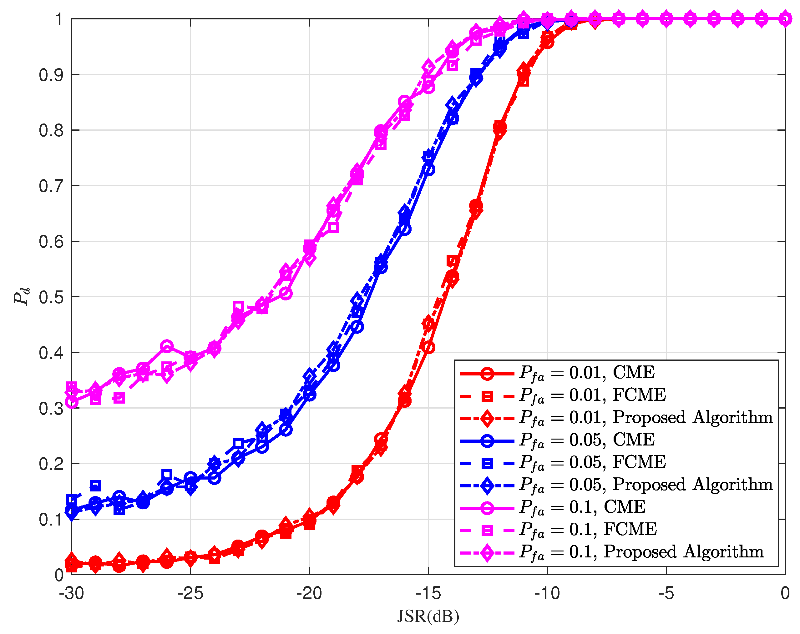
Figure 7 shows the jamming detection probability when there is single-tone jamming. It can be observed from the figure that the detection probability consistently increases with the target false alarm probability. This is because a higher target false alarm probability lowers the detection threshold, enabling the detection of smaller jamming signals and thereby improving the detection probability. However, this also causes non-jamming signals to be more likely to exceed the lower threshold and be mistakenly identified as interference, resulting in an increase in the actual false alarm probability. The detection probability of the proposed algorithm is largely comparable to that of FCME while outperforming CME.
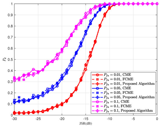
Figure 7.
The detection probability of single-tone jamming in an OTFS system.
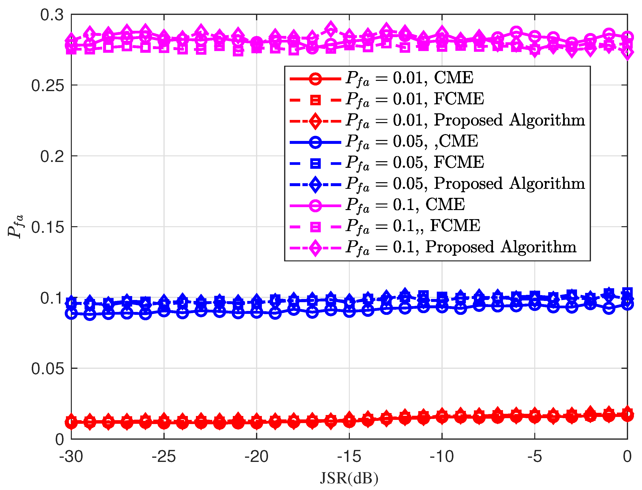
Figure 8 illustrates the false alarm probability under single-tone jamming. The simulation results indicate that the actual false alarm probability is closely aligned with the theoretical results, although the error between them increases as the target false alarm probability rises. The reason is that a high target false alarm probability typically results from a lower decision threshold. However, when a lower threshold factor is applied, the jamming-free signal becomes more susceptible to noise. The smaller the threshold factor, the greater the impact of noise, leading to an increase in the actual false alarm probability. Overall, the performance differences between the three algorithms under single-tone interference are negligible.
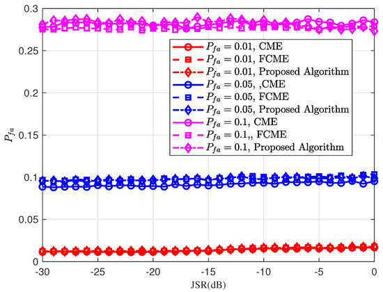
Figure 8.
The false alarm probability of single-tone jamming in an OTFS system.
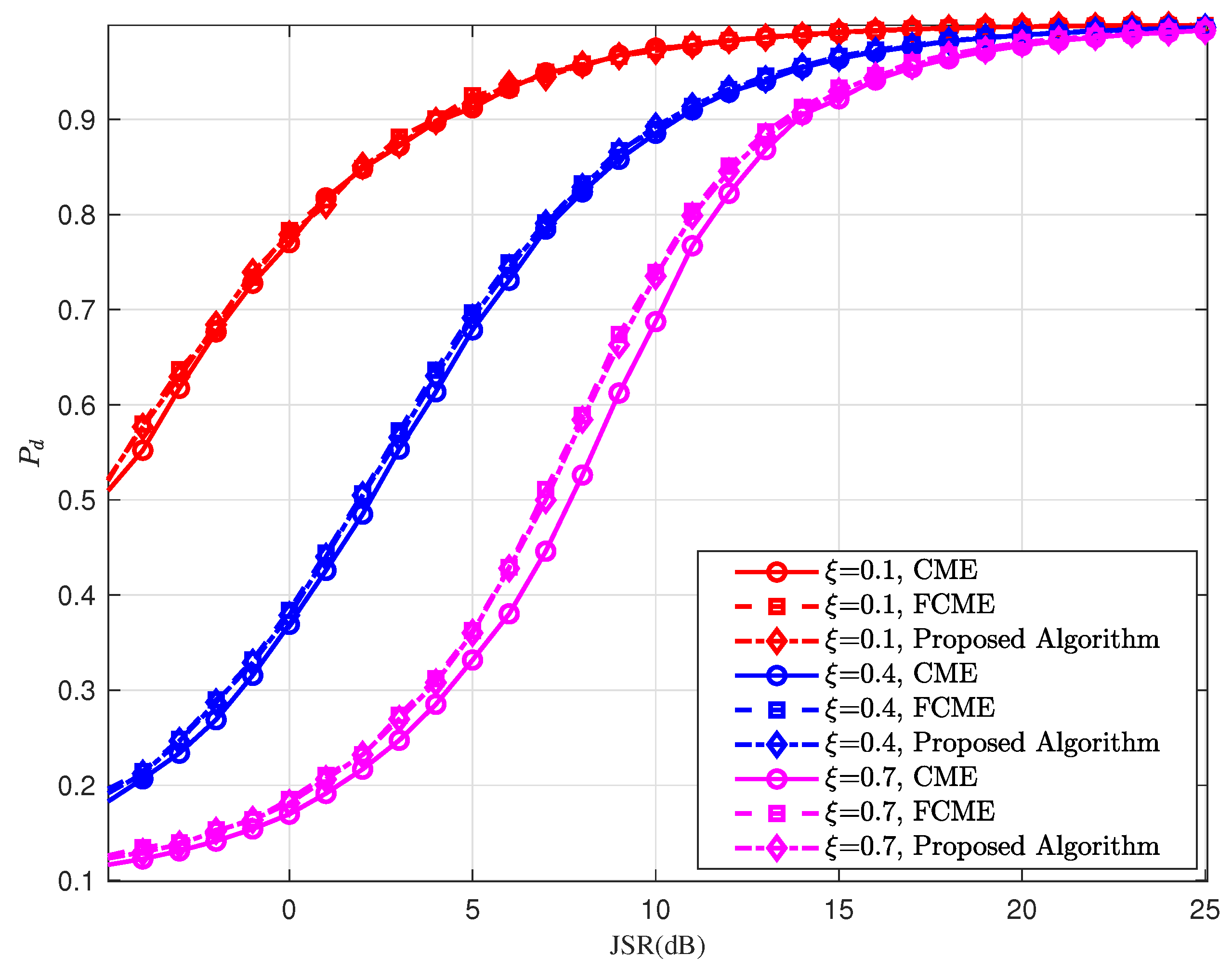
Figure 9 shows the jamming detection probability under partial-band jamming, with a target false alarm probability , and varying jamming factors . In simulations, scenarios of partial-band jamming with are considered. The detection probabilities of three different algorithms, including the proposed method and the conventional CME and FCME algorithms, are compared. For a small jamming factor (e.g., ), the detection performance of the three algorithms is nearly identical. However, as the jamming factor increases, the performance advantages of the FCME and the proposed algorithm become more apparent. As the jamming factor increases, the detection probability performance decreases. The primary reason is that under the same JSR conditions, a larger jamming factor corresponds to a wider jamming bandwidth, resulting in a lower jamming power spectral density. Consequently, the jamming signal becomes more difficult to detect relative to the signal power.
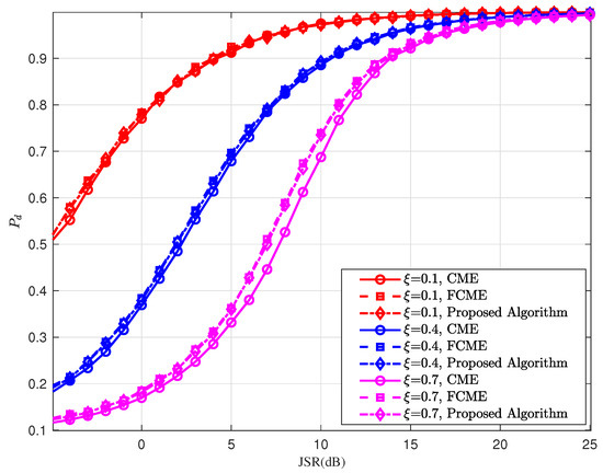
Figure 9.
The detection probability of partial-band jamming in an OTFS system.
In summary, the proposed FCME algorithm demonstrates a performance comparable to that of the conventional FCME algorithm. However, it offers lower computational complexity because the sorting process is significantly reduced during the initialization stage.
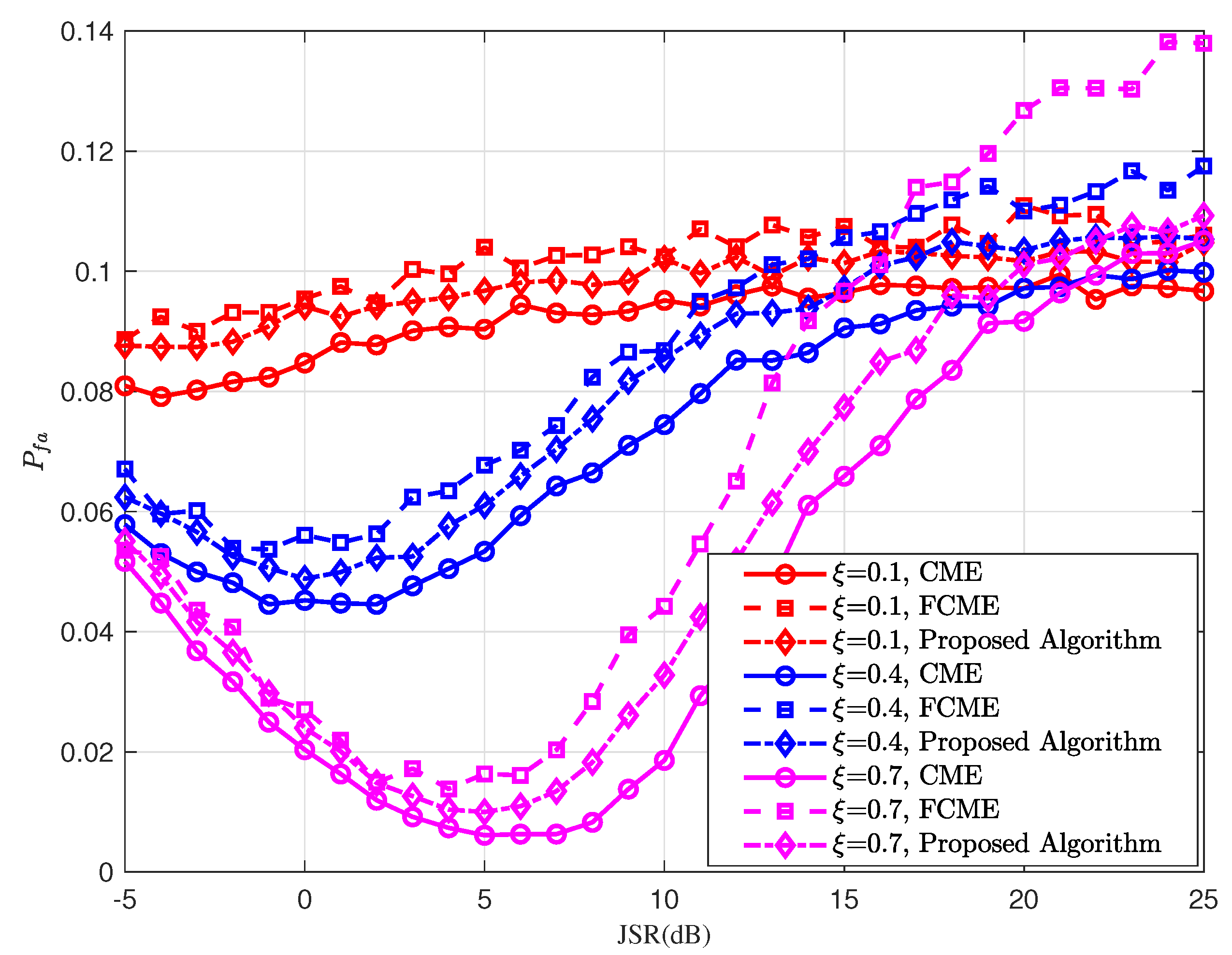
Figure 10 illustrates the actual jamming false alarm probability under partial-band jamming when the target false alarm probability is set to . Compared to the single-tone interference scenario, the actual false alarm probability under partial-band interference deviates noticeably from the theoretical analysis results. Moreover, the behavior of the actual false alarm probability becomes more complex as the jamming factor increases. This phenomenon is caused by the combined effects of noise and partial-band jamming signal. On the one hand, the interplay of noise and jamming increases the randomness of the signal spectrum. On the other hand, the partial-band jamming signals cause the spectral amplitude of the received signal to deviate from the Rayleigh distribution assumed in theoretical analysis. These factors ultimately result in a certain degree of deviation between the theoretical analysis and the actual results.

Figure 10.
The false alarm probability of partial-band jamming in an OTFS system.
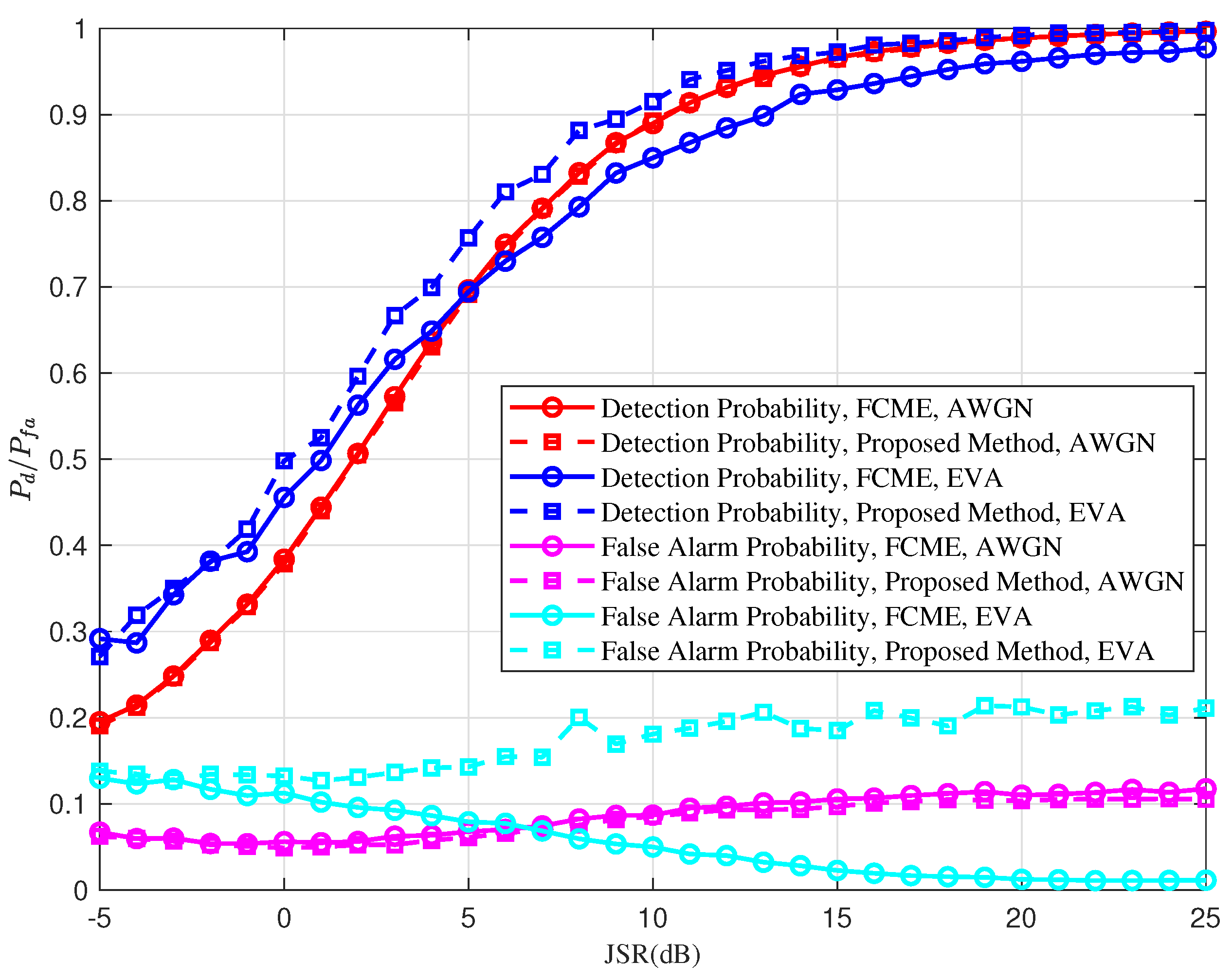
Figure 11 illustrates the detection performance of the conventional FCME and the proposed algorithm under partial-band jamming with a jamming factor of in both AWGN and EVA channels, with a target false alarm probability of . In simulations, the carrier frequency is set to 4 GHz, and the speed of communication terminal is up to 500 km/h. Simulation results show that the proposed FCME algorithm remains effective in the EVA channel. In simulations, the detection probability of the proposed algorithm tends to converge when the JSR is around 15 dB, indicating that jamming detection remains effective in the EVA channel. Additionally, under low JSR conditions, the proposed FCME demonstrates performance comparable to that of the conventional FCME in the EVA channel. Compared to the traditional FCME algorithm, the proposed method exhibits a higher false alarm probability in the EVA channel. The reason is that frequency-selective fading caused by the multipath channel reduces the initialization threshold, leading to an increased likelihood of detecting non-jamming signals as interference.

Figure 11.
The detection performance of conventional FCME and the proposed algorithm under AWGN channel and EVA channel.
4.2. Jamming Suppression Performance
In this subsection, the overall jamming suppression performance is evaluated in terms of BER in both single-tone and partial-band jamming scenarios. In the simulations, the proposed jamming detection algorithm described in Section 3 is utilized, with the target false alarm probability set to .
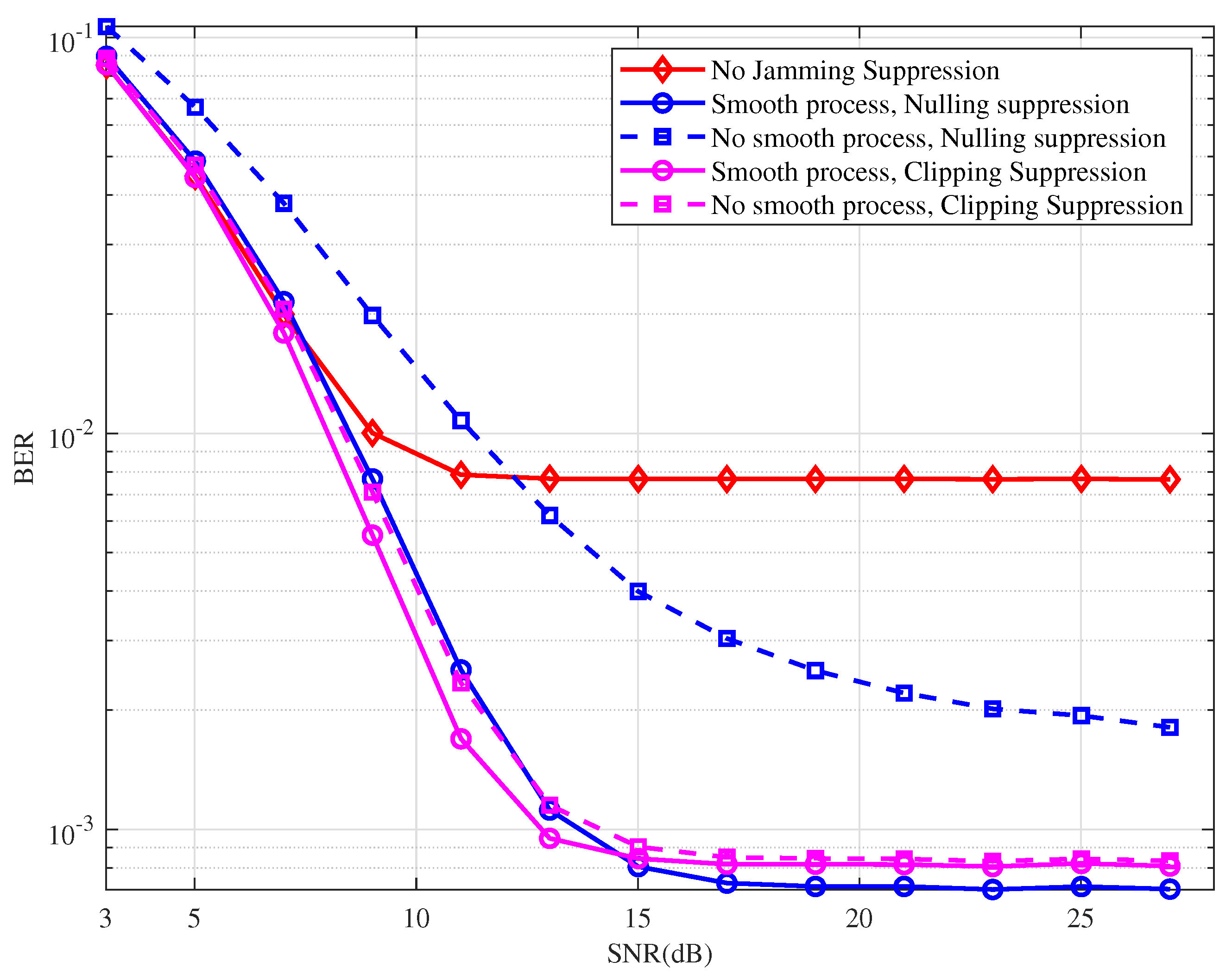
Figure 12 illustrates the BER performance of an OTFS system when the proposed jamming detection method is applied, followed by different jamming suppression algorithms. To enable a more systematic performance comparison, we also evaluated the performance differences in jamming detection with and without the use of a smoothing window. It can be observed that both nulling suppression and clipping suppression improve BER performance regardless of whether the smoothing windowing process is applied. However, when the jamming suppression method is fixed, the introduction of the smoothing windowing technique surely enhances BER performance. This improvement can be attributed to the smoothing window’s ability to create a more uniform amplitude distribution of the signal in the frequency domain, effectively mitigating the adverse effects of noise fluctuations and reducing the false alarm probability. Furthermore, nulling suppression, when combined with the proposed jamming detection method, outperforms other combinations.
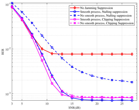
Figure 12.
BER performance of OTFS with different jamming detection and suppression techniques under single-tone jamming.
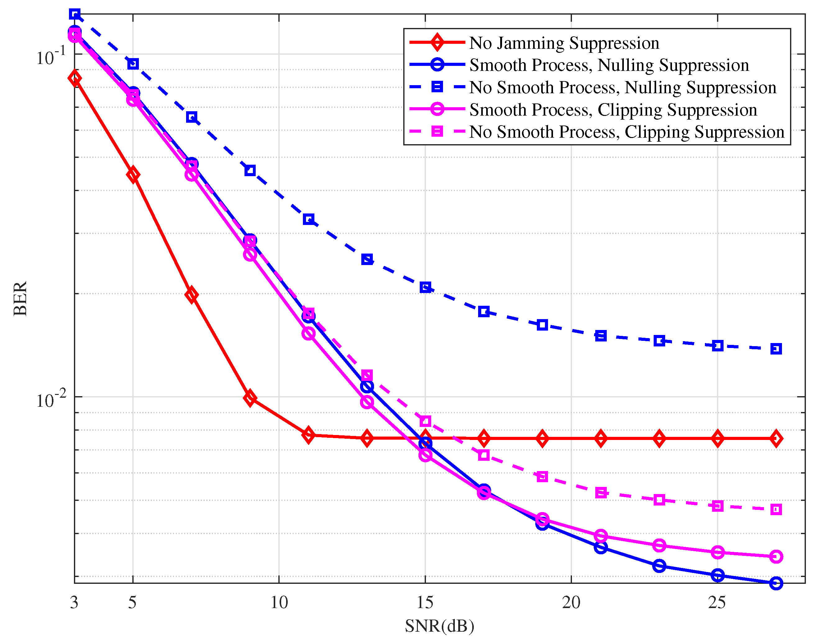
Figure 13 illustrates the BER performance of an OTFS system when the proposed jamming detection method is applied, followed by different jamming suppression algorithms. In the simulations, the partial-band jamming is configured with a JSR of 10 dB and . In the low SNR region, the BER is primarily influenced by noise, and the jamming suppression method fails to effectively mitigate the jamming in the received signal. Similar to the single-tone jamming scenario, the introduction of smoothing windowing significantly enhances the BER performance of both jamming suppression methods when SNR > 13 dB. Additionally, nulling suppression combined with the proposed jamming detection technique outperforms the other methods.
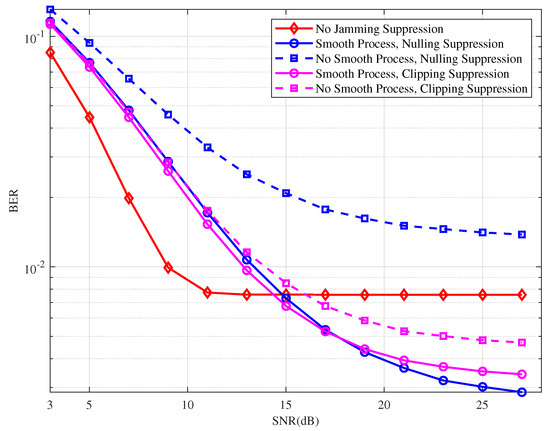
Figure 13.
BER performance of OTFS with different jamming detection and suppression techniques under partial-band jamming.
5. Conclusions
This paper investigates the anti-jamming capabilities of OTFS modulation, focusing on detection and suppression methods in an AWGN channel. A frequency-domain anti-jamming technique was proposed, utilizing a time-domain overlapping window strategy to effectively reduce jamming sidelobes while minimizing the SNR degradation caused by the window function. To further improve jamming detection accuracy, a smoothing window method was introduced, providing stable samples and reducing the false alarm rate significantly. Additionally, a low-complexity improved FCME algorithm was developed, enhancing the practicality and efficiency of interference suppression in real-world applications. Through simulation analyses under single-tone and partial-band jamming scenarios, the proposed methods demonstrated robust performance, validating their effectiveness in complex and jamming-prone environments. These contributions highlight the potential of OTFS modulation as a resilient waveform for high-mobility communication systems, providing insights into its practical deployment in next-generation wireless networks. Following the main results presented here, a promising direction for future work is to extend the proposed methods to more diverse jamming scenarios, such as multitone and adaptive jamming, and to explore their applicability in non-linear and multipath fading channels.
Author Contributions
Conceptualization, L.L. and H.L.; formal analysis, P.W. and J.L.; supervision, L.L.; writing—original draft, P.W. and D.Z.; writing—review and editing, H.L.; funding acquisition, L.L. and H.L. All authors have read and agreed to the published version of the manuscript.
Funding
This work was supported in part by the National Natural Science Foundation of China under Grant 62371037, in part by the China Scholarship Council under Grant Number 202306460096, in part by the Guangdong Basic and Applied Basic Research Foundation under Grant 2024A1515011186 and Grant 2025A1515010082, and in part by the China Postdoctoral Science Foundation under Grant 2023M740223.
Data Availability Statement
The original contributions presented in this study are included in the article. Further inquiries can be directed to the corresponding author.
Conflicts of Interest
The authors declare no conflicts of interest.
References
- Nguyen, D.C.; Ding, M.; Pathirana, P.N.; Seneviratne, A.; Li, J.; Niyato, D.; Dobre, O.; Poor, H.V. 6G internet of things: A comprehensive survey. IEEE Internet Things J. 2022, 9, 359–383. [Google Scholar]
- Wang, Z.; Du, Y.; Wei, K.; Han, K.; Xu, X.; Wei, G.; Tong, W.; Zhu, P.; Ma, J.; Wang, J.; et al. Vision, application scenarios, and key technology trends for 6G mobile communications. Sci. China Inf. Sci. 2022, 65, 1–27. [Google Scholar]
- Su, Y.; Liu, Y.; Zhou, Y.; Yuan, J.; Cao, H.; Shi, J. Broadband LEO Satellite Communications: Architectures and Key Technologies. IEEE Wirel. Commun. 2019, 26, 55–61. [Google Scholar]
- Tataria, H.; Shafi, M.; Molisch, A.F.; Dohler, M.; Sjoland, H.; Tufvesson, F. 6G wireless systems: Vision, requirements, challenges, insights, and opportunities. Proc. IEEE 2021, 109, 1166–1199. [Google Scholar]
- Zhang, Z.; Xiao, Y.; Ma, Z.; Xiao, M.; Ding, Z.; Lei, X.; Karagiannidis, G.; Fan, P. 6G wireless networks: Vision, requirements, architecture, and key technologies. IEEE Veh. Technol. Mag. 2019, 14, 28–41. [Google Scholar]
- Hadani, R.; Rakib, S.; Tsatsanis, M.; Monk, A.; Goldsmith, A.J.; Molisch, A.F.; Calderbank, R. Orthogonal time frequency space modulation. In Proceedings of the 2017 IEEE Wireless Communications and Networking Conference (WCNC), San Francisco, CA, USA, 19–22 March 2017; pp. 1–6. [Google Scholar]
- Das, S.S.; Prasad, R. OTFS: Orthogonal Time Frequency Space Modulation A Waveform for 6G; River Publishers: Aalborg, Denmark, 2022. [Google Scholar]
- Liu, Y.; Chen, M.; Pan, C.; Gong, T.; Yuan, J.; Wang, J. OTFS Versus OFDM: Which is Superior in Multiuser LEO Satellite Communications. IEEE J. Sel. Areas Commun. 2025, 43, 139–155. [Google Scholar] [CrossRef]
- He, R.; Zhang, X.; Cui, Q.; Tao, X. Doppler Interference Analysis for OTFS-Based LEO Satellite System. IEEE J. Sel. Areas Commun. 2025, 43, 75–89. [Google Scholar] [CrossRef]
- Shen, B.; Wu, Y.; Gong, S.; Liu, H.; Ottersten, B.; Zhang, W. Massive MIMO-OTFS-Based Random Access for Cooperative LEO Satellite Constellations. IEEE J. Sel. Areas Commun. 2025, 43, 90–106. [Google Scholar]
- Wang, J.; Jiang, C.; Kuang, L. High-Mobility Satellite-UAV Communications: Challenges, Solutions, and Future Research Trends. IEEE Commun. Mag. 2022, 60, 38–43. [Google Scholar] [CrossRef]
- Hu, J.; Shi, J.; Ma, S.; Li, Z. Secrecy Analysis for Orthogonal Time Frequency Space Scheme Based Uplink LEO Satellite Communication. IEEE Wireless Commun. Lett. 2021, 10, 1623–1627. [Google Scholar] [CrossRef]
- Wang, J.; Jiang, C.; Kuang, L.; Shan, C.; Zhan, C. Second Order Time-Frequency Modulation in Satellite High-Mobility Communications. In Proceedings of the 2020 16th International Conference on Wireless and Mobile Computing, Networking and Communications (WiMob), Thessaloniki, Greece, 12–14 October 2020; pp. 1–5. [Google Scholar]
- Liu, S.; Yang, F.; Song, J.; Han, Z. Block Sparse Bayesian Learning-Based NB-IoT Interference Elimination in LTE-Advanced Systems. IEEE Trans. Commun. 2017, 65, 4559–4571. [Google Scholar]
- Wei, Z.; Yuan, W.; Li, S.; Yuan, J.; Bharatula, G.; Hadani, R.; Hanzo, L. Orthogonal Time-Frequency Space Modulation: A Promising Next-Generation Waveform. IEEE Wirel. Commun. 2021, 28, 136–144. [Google Scholar] [CrossRef]
- Guo, Q.; Jiang, H.; Xiang, J.; Zhong, Y. An Energy Concentration Narrowband Interference Suppression Algorithm for OTFS Systems. IEEE Commun. Lett. 2023, 27, 3360–3364. [Google Scholar] [CrossRef]
- Alsalameh, H.; Develi, I.; Karahan, B. BER Performance Analysis of OTFS-IM Systems under Barrage Jamming. In Proceedings of the 2024 IEEE International Conference on Contemporary Computing and Communications (InC4), Bangalore, India, 15–16 March 2024; pp. 1–5. [Google Scholar]
- Deka, K.; Thomas, A.; Sharma, S. OTFS-SCMA: A codedomain NOMA approach for orthogonal time frequency space modulation. IEEE Trans. Commun. 2021, 69, 5043–5058. [Google Scholar]
- Bai, Z.; Li, B.; Yang, M.; Yan, Z.; Zuo, X.; Zhang, Y. FH-SCMA: Frequency-hopping based sparse code multiple access for next generation Internet of Things. In Proceedings of the 2017 IEEE Wireless Communications and Networking Conference (WCNC), San Francisco, CA, USA, 19–22 March 2017; pp. 1–6. [Google Scholar]
- Deng, Q.; Ge, Y.; Ding, Z. Jamming Suppression via Resource Hopping in High-Mobility OTFS-SCMA Systems. IEEE Wireless Commun. Lett. 2023, 12, 2138–2142. [Google Scholar]
- Xu, H.; Cheng, Y.; Wang, P. Jamming Detection in Broadband Frequency Hopping Systems Based on Multi-Segment Signals Spectrum Clustering. IEEE Access 2021, 9, 29980–29992. [Google Scholar] [CrossRef]
- Henttu, P.; Aromaa, S. Consecutive mean excision algorithm. In Proceedings of the IEEE Seventh International Symposium on Spread Spectrum Techniques and Applications, Praha, Czech Republic, 2–5 September 2002; pp. 450–454. [Google Scholar]
- Saamisaari, H.; Henttu, P. Impulse detection and rejection methods for radio systems. In Proceedings of the IEEE Military Communications Conference (MILCOM), Boston, MA, USA, 13–16 October 2003; pp. 1126–1131. [Google Scholar]
- Lehtomaki, J.J.; Vartiainen, J.; Juntti, M.; Saarnisaari, H. CFAR outlier detection with forward methods. IEEE Trans. Signal Process. 2007, 55, 4702–4706. [Google Scholar] [CrossRef]
- Vartiainen, J.; Lehtomaki, J.J.; Saarnisaari, H. Double-threshold based narrowband signal extraction. In Proceedings of the 2005 IEEE 61st Vehicular Technology Conference, Stockholm, Sweden, 30 May–1 June 2005; pp. 1288–1292. [Google Scholar]
- Vartiainen, J.; Sarvanko, H.; Lehtomaki, J.; Juntti, M.; Latvaaho, M. Spectrum sensing with LAD-based methods. In Proceedings of the 2007 IEEE 18th International Symposium on Personal, Indoor and Mobile Radio Communications, Athens, Greece, 3–7 September 2007; pp. 1–5. [Google Scholar]
- Jia, K.X.; He, Z.S. Narrowband signal localization based on enhanced LAD method. J. Commun. Netw. 2011, 13, 6–11. [Google Scholar]
- Press, W.H.; Teukolsky, S.A.; Vetterling, W.T.; Flannery, B.P. Numerical Recipes in C; the Art of Scientific Computing; Cambridge University Press: Cambridge, UK, 1992. [Google Scholar]

Disclaimer/Publisher’s Note: The statements, opinions and data contained in all publications are solely those of the individual author(s) and contributor(s) and not of MDPI and/or the editor(s). MDPI and/or the editor(s) disclaim responsibility for any injury to people or property resulting from any ideas, methods, instructions or products referred to in the content. |
© 2025 by the authors. Licensee MDPI, Basel, Switzerland. This article is an open access article distributed under the terms and conditions of the Creative Commons Attribution (CC BY) license (https://creativecommons.org/licenses/by/4.0/).