Oriented Data Generation for Power System Transient Stability Boundary Exploration Based on Support Vector Machine

Abstract

Transient stability boundary is an important tool for the security and stability analysis of power systems, but typically, obtaining it will result in a high computational burden. Existing methods for obtaining transient stability boundary often involve grid scanning, which generates a large number of dense operating points, followed by transient simulation, which incurs substantial time costs. This paper proposes a method for transient stability boundary exploration based on a Support Vector Machine (SVM), which uses a small number of operating points to obtain a more precise stability boundary while efficiently and accurately acquiring stable operating points near the stability boundary. Firstly, the SVM is employed to classify the initial samples and determine the transient stability boundary under the N-1 fault. Secondly, re-sampling is conducted for operating points near the stability boundary determined by the initial samples. After updating the sample set, SVM classification is performed again. This process is iterated multiple times, and the operating points are continuously generated in the direction oriented toward the actual stability boundary while obtaining a more precise transient stability boundary under the N-1 fault. Finally, the proposed method is validated using actual operational data from a regional power grid of China Southern Power Grid (Guangzhou, China), demonstrating the accuracy and efficiency of the proposed approach.

1. Introduction

Power system stability control strategies are an important means to ensure the safe and stable operation of the power grid when it suffers from severe faults. When the power grid is subjected to severe faults (such as a bipolar block of high voltage direct current (HVDC), double-circuit tripping of lines, etc.), it is necessary for the pre-designed and deployed stability control devices to quickly implement stability control measures in order to maintain the safe and stable operation of the system. To fully exert the role of the above-mentioned stability control devices, it is necessary to optimize their setting values and formulate relevant operating regulations [1].

In China, with the vigorous advancement in new power system construction, the “dual-high” characteristics of power systems (high proportion of renewable energy access and high proportion of power electronic equipment application) are becoming increasingly prominent, posing severe challenges to the safe and stable operation of power grids [2,3]. At present, power grid stability control strategies are based on the typical system operating modes for fault set scanning and the construction of relatively conservative stability control measures. However, with the gradual advancement of new power systems, the power grids’ flow patterns have become more diverse [4], continuously compressing the originally relatively conservative operating space. Therefore, the relevant departments of power grid companies need to regularly validate the setting values of stability control devices and correct the stability control setting values that do not meet the operating modes of the coming year. In China Southern Power Grid, it is necessary to conduct a stability control strategy setting value validation for the next three years to ensure that the power system can still maintain safe and stable operation under severe faults.

In the actual operation of power systems, a power grid is required to be able to maintain stable operation in the event of an N-1 fault. When an N-2 fault occurs, and if the power grid experiences stability issues, the power system is required to be able to maintain stable operation after implementing corresponding stability control strategies. Therefore, to simulate various scenarios in actual production and in the task of stability control setting value validation of power systems, a large number of operating points are often generated using a method similar to grid scanning. After obtaining the stable operation range under the N-1 fault, the operating points within this range are scanned under the N-2 fault sets, and the corresponding stability control strategies are calculated and compared with the previous setting values.

As indicated by the above discussion, the task of stability control setting value validation in a power system is of utmost importance but involves a substantial computational burden, which is primarily due to the generation of a vast number of operating points and transient simulations. To avoid the significant investment of human effort and time, data-driven technologies can be employed to replace transient simulations. On the other hand, screening the operating points that need to be validated can also save time and computational resources for the validation task. This is because even when using data-driven technologies for stability control setting value validation in a power system, the time required to generate the operating points can exceed the time needed for the validation task itself when using traditional transient simulation if a large number of sample points are validated. Actually, the existing applications of artificial intelligence technologies in power system transient stability assessment have become relatively mature. Reference [5], addressing the issues of high computational burden and poor performance robustness in transient stability assessment, designed a priority strategy based on information entropy to distinguish samples with high information content, dynamically scheduling data-driven transient stability batch assessment task queues and updating models in a timely manner, thereby further reducing simulation time. Reference [6], in response to the problem of model assessment performance degradation due to changes in operating points during actual power grid operation, proposed a bidirectional active transfer learning framework, which combines forward active learning and backward active learning. And by actively selecting the most worthwhile instances to label under new operating conditions and actively removing the most useless instances under original operating conditions, a hybrid instance set was constructed to adapt to new operating conditions. Therefore, this paper focuses on quickly obtaining the stability boundary (the critical dividing line between stable and unstable operating states, determined through transient simulations by adjusting the output combinations of key variables such as power plant generation and DC transmission power) under the N-1 fault and a large number of stable operating points near the boundary to improve the efficiency of power system stability control setting value validation.

To address the issue of the massive computational burden associated with validation tasks, data-driven technologies are typically employed to accelerate this process. Although there are currently no studies that directly apply these technologies to the validation of power system stability control setting value, data-driven-based validation tasks are essentially similar to transient stability assessment. In fact, a validation task for power system stability control setting values is essentially transient stability assessment with stability control strategies. Therefore, current research related to transient stability assessment can provide insights into the validation task for stability control setting values. However, unlike transient stability assessment, power system stability control setting value validation requires scanning all operating points within the stable operation range of the N-1 fault for the N-2 fault. In theory, the number of operating points that the validation task needs to scan is infinite.

When using data-driven technologies for the validation of power system stability control setting values, the time required to generate these sample points can exceed the time needed for validation tasks using traditional transient simulation if almost all the sample points are validated. In practice, based on experience and prior knowledge, the most severe instability cases under the N-2 fault occur at the stable operation boundaries under the N-1 fault. Since only one unstable point needs to be found to conclude that the existing setting value does not meet the stability conditions, focusing on validating these boundary operating points can accelerate the setting value validation task. Therefore, quickly identifying the stable boundary under the N-1 fault and obtaining a large number of stable sample points near the boundary helps improve the efficiency of the power system stability control setting value validation.

To address the issue of determining stability boundaries, existing studies have leveraged artificial intelligence technologies to accelerate this process. For example, Reference [7] applies modern statistical nonparametric methodology to the problem of transient stability boundary prediction in large-scale power engineering systems. By applying nonparametric kernel estimation methods to hypothesized additive models, it derives an easily interpretable boundary prediction algorithm, thereby avoiding the curse of dimensionality. Reference [8] employs a synchronous variable selection and estimation method, resulting in a transient stability boundary prediction model with significantly reduced complexity. Reference [9] models the transient stability boundary as a nonlinear mapping between the system parameters of interest and the corresponding critical clearing times, addressing the issue of the lack of transient stability boundary analysis and description capabilities for multiple operating states and unexpected events in power systems. Reference [10] simplifies the theoretical basis of the trajectory reversal expansion method based on Lyapunov functions and significantly improves the stability boundary with moderate computational costs by relaxing the requirement that the initial guess is a subset of the stability region. Reference [11] proposes a method based on collocation methods for polynomial approximation and sensitivity analysis to partition stable and unstable subspaces. In fact, most of the above studies determine the transient stability boundary of power systems by improving models or enhancing the stability characteristics of samples, but they do not achieve the goal of obtaining the transient stability boundary based on as few sample points as possible.

To address the oriented generation of operating points toward the stability boundary, existing studies have employed data augmentation techniques. Specifically, Reference [12] utilizes a binary search algorithm to iteratively enhance the dataset. Additionally, references [13,14] apply importance sampling techniques within an iterative framework to identify sample points near the transient stability boundary, thereby increasing the number of samples located on the stability boundary. Reference [15] presents the concept of Graph-based Local Re-sampling of perceptron-like neural networks with random projections, which aims to regularize the yielded model. Reference [16] proposes an improved Generative Adversarial Network integrated with transfer learning, which can significantly enhance data generation performance and augment the original dataset. Reference [17] applies Conditional Generative Adversarial Networks to generate unstable samples, balancing the training data. Although the above studies can expand the sample set, most of them obtain operating points from the already generated operating points or through continuous “trial and error”, and have not yet achieved the function of directly generating operating points near the stability boundary.

In summary, to expedite the validation task, it is necessary to rapidly and accurately determine the stability boundary under the N-1 fault, using as few operating points as possible, and to generate operating points oriented toward the stability boundary, which can then be used for subsequent N-2 fault analysis. Given that the stability boundary serves as the critical dividing line between stable and unstable operating points, it is essentially necessary to identify a methodology that enables the rapid classification of operating points, thereby facilitating the determination of the stability boundary.

Considering that existing studies have not achieved the goal of obtaining the transient stability boundary by using a small number of operating points, and directly sampling operating points near the stability boundary, SVM stands out for its ability to efficiently handle scenarios with few samples and high dimensionality as well as its strong interpretability and excellent generalization performance. This paper employs an SVM to determine the stability boundary of power systems under the N-1 fault and implements re-sampling, providing critical samples for strategy calculation under the N-2 fault, thereby accelerating the validation task of power system stability control setting value.

Inspired by References [18,19], the main contributions of this paper are as follows:

(1)

Initial Guess Stability Boundary Exploration with Limited Samples: Based on the SVM, we propose a method to determine the initial guess transient stability boundary under the N-1 fault, which can efficiently identify the stability boundary, even with limited data, thereby providing a robust foundation for further stability analysis.

(2)

Enhanced Stability Boundary Refinement and Data Augmentation: Re-sampling is conducted to generate more samples oriented toward the stability boundary, and a more precise stability boundary is re-determined. Importantly, the newly generated samples near the stability boundary are identified as critical objects for stability assessment under the N-2 fault conditions in subsequent research. This not only enhances the robustness of the stability boundary exploration but also provides valuable data for extended analysis of more severe fault scenarios.

The remainder of this paper is organized as follows. Section 2 presents the problem statement and necessary notations; Section 3 shows our main research ideas and principles; Section 4 reports the case studies on a regional power grid of China Southern Power Grid; finally, Section 5 concludes the paper.

2. Problem Statement

In the actual operation of a power system, the stability of a region is influenced by numerous factors, such as the power output of power plants, the power of direct current (DC) transmission, and the topology of transmission lines. The topology of transmission lines does not change for a certain amount of time, while the power output of power plants and the power of DC transmission vary with changes in operating points, significantly affecting the stability of the region. For transient stability analysis of power systems subjected to large disturbances, the electromechanical transient model is generally employed for analysis, which can be described by the following differential-algebraic equations:

$$\left\{\begin{array}{c}{\displaystyle \frac{\mathrm{d}x}{\mathrm{d}t}}=f(x,y)\\ 0=g(x,y)\end{array}\right.$$

(1)

For simple systems, when the generator is represented by a classical second-order model, the generator model in Equation (1) can be expressed as follows:

$$\left\{\begin{array}{l}{\displaystyle \frac{\mathrm{d}\delta }{\mathrm{d}t}}=\omega -{\omega }_0\hfill \\ T_J{\displaystyle \frac{\mathrm{d}\omega }{\mathrm{d}t}}=P_T-P_E\hfill \end{array}\right.$$

(2)

where P_T represents the mechanical power output of the prime mover (which is also the generator power), and $P_E={\displaystyle \frac{E^{\prime }U}{x}}\mathrm{s}\mathrm{i}\mathrm{n}\delta$ represents the electromagnetic power transmitted from the generator. When a short-circuit fault occurs in a certain area, the reactance x increases, leading to a decrease in P_E, which disrupts the original transient stability. At this point, by reducing the power output P_T of the generator unit or tripping the generator, the system can be brought back to a stable operating point.

Actually, the generator tripping strategy mentioned above is one of the stability control strategies in power systems, and it can be represented by the following formula:

$$\left\{\begin{array}{ll}DP=0\hfill & P_{\mathrm{xhs}}<P_{\mathrm{mk}\_\mathrm{set}}\hfill \\ DP=K_{\mathrm{n}}(P_{\mathrm{xhs}}-P_{\mathrm{set}\_\mathrm{n}})\hfill & P_{\mathrm{xhs}}\ge P_{\mathrm{mk}\_\mathrm{set}}\hfill \\ t_{\mathrm{op}}\le t_{\mathrm{set}}\hfill & \end{array}\right.$$

(3)

where DP is the calculated generator tripping amount, P_{mk_set} is the tripping threshold setting value, P_xhs is the transmission power of the corresponding line, K_n is the coefficient for the required tripping amount, P_{set_n} is the base value for the required tripping amount that switches with the operating point, t_op is the operating time, and t_set is the specified maximum operating time. These values are the aforementioned setting values of the stability control device. In practice, reasonable setting values can not only ensure the stability of the system but also minimize the system’s losses under fault conditions.

Before conducting the task of power system stability control setting value validation, it is necessary to determine the stable operating range of the system under the N-1 fault. We take the simplest region containing one power plant and one DC transmission corridor as an example. As shown in Figure 1, the region includes a large thermal power plant G1, and a DC transmission corridor C1-C2. It is worth noting that the power output of G1 and the transmission power of the corridor C1-C2 are subject to maximum and minimum power output constraints.

In different operating points, the stability of the region varies accordingly. For instance, when power plant G1 is operating at full capacity and the DC transmission corridor is fully loaded, a line disconnection fault between G1 and C1 can lead to an overloading of the G1-Gan line and instability of the power angle of G1. Under such circumstances, to ensure stable operation under the N-1 fault in the region, it is necessary to impose constraints on the power output of power plant G1 and the power of the DC transmission corridor C1-C2. Therefore, the output power of power plant G1 and the DC transmission corridor C1-C2 are subject to the following constraints:

$$\left\{\begin{array}{l}{P}_{\mathrm{Gmin}}\le P_{\mathrm{G}1}\le P_{\mathrm{Gmax}}\hfill \\ \begin{array}{l}{P}_{\mathrm{DCmin}}\le P_{\mathrm{C}1\_\mathrm{C}2}\le P_{\mathrm{DCmax}}\\ P_{\mathrm{delmin}}\le P_{\mathrm{G}1}-P_{\mathrm{C}1\_\mathrm{C}2}\le P_{\mathrm{delmax}}\end{array}\hfill \\ \mathrm{for} t \mathrm{in} \mathrm{the} \mathrm{entire} \mathrm{time} \mathrm{domain}\hfill \end{array}\right.$$

(4)

where P_G1 is the actual power output of the power plant; P_{C1_C2} is the DC transmission power, P_Gmin and P_Gmax are the minimum and maximum power outputs of power plant G1; P_DCmin and P_DCmax are the minimum and maximum transmission powers of the DC corridor C1-C2; P_delmin and P_delmax are the specified minimum and maximum differences between the power plant output and the DC transmission power. The above constraints should be satisfied for the entire time domain.

Figure 2 shows the results of the N-1 fault transient simulation for sample points obtained through grid scanning of the region. Two pieces of information can be gleaned from the figure: first, the stable operating range under the N-1 fault is reduced, and unstable operating points (such as those corresponding to the orange points) should be avoided in actual production; second, the stability boundary is nonlinear, making it difficult to quickly obtain based on manual experience.

If the transient stability boundary is obtained through traditional grid scanning, for each given base mode (the number of points is denoted as N1), it is necessary to consider various line maintenance modes (denoted as N2) and then set various fault types and locations (the number is denoted as N3). Finally, for each of the N1 × N2 × N3 scanning analysis tasks, it is necessary to adjust the total active power output of key substations and the direct current transmission power to form a set of scenarios.

Therefore, to avoid the substantial time cost associated with grid scanning, this paper employs SVM technology to rapidly identify the stability boundary with a limited number of samples. To enhance the precision of the stability boundary, continuous re-sampling near the boundary and updating the sample set should be conducted after obtaining the initial stability boundary. Then, by utilizing the SVM to search for the stability boundary with the updated sample set again, a more accurate boundary can be achieved.

In fact, the stability boundary under the N-2 fault with stability control strategies, compared to N-1, undergoes changes in shape and position. Their positional relationship can be categorized into two scenarios: first, the former boundary expands outward beyond the latter; second, the former boundary contracts inward. As shown in Figure 3, the blue curve represents the stability boundary under the N-1 fault, while the orange curve represents the stability boundary under the N-2 fault with stability control strategies.

For all points that satisfy stable operation under the N-1 fault (such as the operating points marked in Figure 3), stability cannot be guaranteed under the N-2 fault with stability control strategies. However, it can be observed from the figure that, under the premise of stable operation satisfying the N-1 fault, if there exists an operating point that remains unstable after stability control measures are taken under the N-2 fault (here, we ideally assume that all unstable operating points are near the boundary), it is certain that a point closest to this operating point can be found on the stability boundary under the N-1 fault (blue curve). That is, in Figure 3, there are some segments of the blue curve and their nearby small ranges where the operating points are farthest from the orange curve (the operating points with the most severe instability after taking stability control strategies under the N-2 fault). Therefore, the aforementioned re-sampling near the stability boundary under the N-1 fault serves two purposes: first, to accelerate the acquisition of a more precise stability boundary; second, to generate a large number of critical samples for subsequent stability control setting value validation tasks.

3. Support Vector Machine-Based Oriented Data Generation

In this section, the SVM-based stability boundary exploration method, as well as the principle of re-sampling in the direction oriented toward the actual stability boundary, are introduced. Additionally, the principle of the scenario batch generation used in this study is also briefly mentioned.

3.1. Framework

As mentioned above, the overall framework of this research is as follows: (1) Automatically generate operating points by industrial software and perform transient simulation under the N-1 fault to obtain the stability of each operating point. (2) Utilize the SVM to classify the operating points to identify the stability boundary under the N-1 fault. (3) Re-sample the samples near the stability boundary, perform transient simulation, and update the sample set. (4) Reclassify the updated sample points using the SVM to obtain a more precise stability boundary. (5) Repeat the above process until the precision of the boundary meets the expected value or the number of iterations reaches the set value N. (6) Save the stable operating points near the stability boundary as sample inputs for subsequent stability assessment under the N-2 fault with stability control strategies.

The overall framework of this study is shown in Figure 4.

3.2. Operating Point Batch Generation

In actual production, the generation of operating points requires manual adjustment, which is not conducive to the automated operation of the program. Therefore, before determining the stability boundary and re-sampling, the batch automatic generation of operating points and the batch transient simulation is a must so that the stability assessment is achieved automatically.

Inspired by Reference [20], the key steps for the batch generation of operating points are as follows:

(1)

Combination customization of scenario sets. Taking the simplest two-variable system (as shown in Figure 1) as an example, it is assumed that the output of power plant G1 is X, and the power of DC transmission corridor C1-C2 is Y. In actual operation, different values of X and Y are subject to different constraints. Here, a local linearization approach [21,22] is adopted, and flexible search rule setting values are achieved through linear combination constraints within finite intervals. These search rules and parameters can be set by experts based on domain knowledge. Generally, the expression for linear constraints is as follows:

$$Z=aX+bY$$

(5)

where Z ∈ [Zmin, Zmax] represents the search boundary. In the process of generating operating points based on such constraints, the horizontal search step size SX is first specified. Within the range of values for X, all possible values of X are traversed. Subsequently, for the vertical search step size SZ, all possible values of Z within the search boundary range are traversed. For each value of Z, the corresponding value of Y is determined. Thus, the values of X and Y for each scenario can be obtained. For the spatial search of multi-dimensional operating modes, a stratified sampling method can be employed, which is not further detailed here.

(2)

Generator power allocation method. Under the conditions of the same critical section power, the same fault, and the same stability control strategy, the different characteristics of generators, the fixed actual cutting machine sequence of the stability control strategy, and the logic of executing whole-machine cutting during actual stability control actions can have a certain impact on the system stability after the stability control action. To ensure the conservativeness of the stability control strategy, the most unfavorable power allocation method for the key generator nodes after stability control is considered here, as well as the method of minimizing the power generation of the generating set involved in regulation. The optimization model is as follows:

$$\begin{array}{l}\min {\displaystyle \sum _{i=1}^n{a}_i\times P_i}\\ \begin{array}{c}\\ \begin{array}{c}\mathrm{s}.\mathrm{t}.\\ \end{array}\\ \\ \end{array} \left\{\begin{array}{l}{\displaystyle \sum _{i=1}^n{P}_i}=P_{\mathrm{total}}\\ P_{\min ,i}\le P_i\le P_{\max ,i}\hfill \\ N_{\min }\le {\displaystyle \sum _{i=1}^n{a}_i}\le N_{\max }\hfill \\ a_i\in \left\{0,1\right\}(i\in 1,2,\dots ,n)\hfill \end{array}\right.\end{array}$$

(6)

where a_i represents whether the i-th unit is operational, and a_i = 1 indicates that the unit is operational; P_i is the power output of the i-th generator; n is the total number of generators participating in the regulation; P_total is the total power output of the units; P_max,i and P_min,i are the maximum and minimum power outputs of the i-th unit; N_max and N_min are the maximum and minimum number of operational generator sets.

The functionalities implemented by the program mentioned in this subsection are shown in Figure 5.

3.3. SVM-Based Stability Boundary Exploration

The SVM is a typical machine learning algorithm used for solving binary and multi-class classification problems. Its core idea is to find an optimal hyperplane in the feature space that maximizes the margin between different classes. The SVM employs the principle of structural risk minimization and utilizes kernel tricks to transform nonlinear problems into linear ones in high-dimensional spaces, thereby addressing issues such as overfitting and the curse of dimensionality. In the context of power system stability control setting value validation, where the goal is to use as few samples as possible, the SVM demonstrates unique advantages in handling small sample sizes, nonlinearity, and high-dimensional pattern recognition. Therefore, this study adopts the SVM for binary classification (stable and unstable) to obtain the stability boundary under the N-1 fault with minimal samples.

The fundamental principle of the SVM is to maximize the margin between samples of different classes through a hyperplane f(x), thereby accomplishing the classification task. The hyperplane f(x) can be expressed as follows:

$$f(x)=w^{T}x+b$$

(7)

where w is the normal vector, which determines the orientation of the hyperplane; b is the bias, which determines the distance between the hyperplane and the origin. For the determination of the hyperplane, the following optimization model is commonly employed:

$$\begin{array}{l}\underset{w,b,{\xi }_i}{\min }{\displaystyle \frac{1}{2}}{‖w‖}^2+C{\displaystyle \sum _{i=1}^l{\xi }_i}\\ \begin{array}{c}\mathrm{s}.\mathrm{t}.\\ \end{array}\left\{\begin{array}{l}{y}_i(w^T{x}_i+b)\ge 1-{\xi }_i\hfill \\ {\xi }_i\ge 0,i=1,2,\dots l\hfill \end{array}\right.\end{array}$$

(8)

where C is the regularization parameter, which controls the trade-off between maximizing the margin and minimizing the classification errors. A larger C tends to reduce classification errors, while a smaller C allows more classification errors to achieve a larger margin. ξ_i > 0 represents the slack variable for the i-th sample, indicating the degree of relaxation for that sample. The term $C{\mathsf{\Sigma }}_{i=1}^l{\xi }_i$ serves as the penalty term.

Given the nonlinear nature of the stability boundary under the N-1 fault in power systems, the kernel trick of the SVM is employed to map samples into a high-dimensional feature space, thereby enabling nonlinear classification and accurately identifying the stability boundary.

Commonly used kernel functions generally include four types, namely linear kernel, polynomial kernel, radial basis function (RBF) kernel, and sigmoid kernel. Given that the stability of power systems in actual operation is related to multiple variables and involves high-dimensional spaces, and the RBF kernel offers significant advantages over other kernels in handling high-dimensional, nonlinear scenarios and requires fewer tuning parameters, this study employs the RBF kernel for the SVM after conducting tests on four kernel functions. The expression for the RBF kernel is as follows:

$$k(x,x^{\prime })=\exp \{-{\displaystyle \frac{{‖x-x^{\prime }‖}^2}{2{\sigma }^2}}\}$$

(9)

So far, the SVM model has been constructed and is capable of performing preliminary classification of the samples. Using the generated operating points and their corresponding stability conclusions as inputs, the stability boundary can be preliminarily obtained.

3.4. Critical Data Re-Sampling

When the number of samples is limited, the stability boundary obtained based on the SVM often exhibits significant errors. To efficiently obtain a more precise stability boundary, re-sampling should be conducted for samples near the boundary (referred to as critical samples) to expand the sample set in the direction oriented toward the actual stability boundary and then reapply the SVM to identify the stability boundary. Based on this, this paper proposes a re-sampling scheme to rapidly expand critical samples.

When conducting the k-th round of classification, the generated sample set is denoted as Ω_k. After performing SVM classification in the k-th round, the stable sample points closest to the stability boundary can be obtained, denoted as Φ_k. Since the scenario generation process involves scanning in both horizontal and vertical directions with step sizes S_X and S_Z, respectively, we center on each element in Φ_k and generate eight surrounding samples based on a step size V. After performing this operation for all elements in Φ_k, the newly obtained sample set is denoted as φ_k. Subsequently, the sample sets are merged to form Ω_k+1 = Ω_k ∪ φ_k, which is used for the (k + 1)-th round of classification. The calculation method for the step size V is as follows:

$$V_{m,k}=\left\{\begin{array}{ll}0.5S_m\hfill & ,k=1\hfill \\ 0.5V_{m,k-1}\hfill & ,k\ge 2\hfill \end{array}\right.$$

(10)

where $m\in \{x,z\}$ and V_m,k denotes the re-sampling step size along direction m in the k-th round. In the first round of re-sampling, the step size V_m,1 is set to 0.5 S_m. When k ≥ 2, a binary division approach is adopted, and the step size is updated as V_m,k = 0.5 V_m,k-1. In order to ensure that at least half of the invalid region between two stability-known operating points is eliminated in each iteration, to rapidly locate the target position within the ordered data, and to avoid local optima, here the re-sampling step size coefficient is designed based on a concept analogous to the binary search method, where each step size is chosen as 0.5 times the previous one.

So far, based on re-sampling, we have achieved the continuous refinement of the stability boundary obtained based on the SVM. After a predetermined number of N iterations, we can obtain a more precise stability boundary and calculate its accuracy (ACC).

For the determination of ACC, the following approach is adopted:

(1)

A fine-grid scanning method is employed to obtain a large number of sample points. Then, transient simulations are performed on these samples to obtain stability labels.

(2)

For all samples located on the stability boundary, a “circle” with radius R (the value of which is related to the required level of conservativeness of the results) is drawn around each sample.

(3)

The stability boundary obtained based on the SVM and all “circles” from step 2 are plotted on the same graph.

(4)

The sample points in the following four scenarios (as shown in Figure 6) are counted and denoted as N₁, N₂, N₃, and N₄, respectively: (a) The stability boundary is outside the circle and close to the stable region. (b) The stability boundary is inside the circle and close to the stable region. (c) The stability boundary is inside the circle and close to the unstable region. (d) The stability boundary is outside the circle and close to the unstable region.

(5)

The accuracy is calculated using the following formula:

$$\mathrm{ACC}={\displaystyle \frac{w_1{N}_1+w_2{N}_2+w_3{N}_3+w_4{N}_4}{N_1+N_2+N_3+N_4}}\times 100\%$$

(11)

where w₁, w₂, w₃, and w₄ are weighting coefficients, which can be determined based on the required level of conservativeness of the results.

4. Case Studies

This section employs actual operational data from a regional power grid of China Southern Power Grid (as shown in Figure 1) for case studies. It is important to note that the case studies presented here are merely illustrative of the proposed method and do not imply that the method is exclusively applicable to the specific case of the China Southern Power Grid. On the contrary, the proposed approach is generalizable and can be applied to any power system. Here, we integrate the program with the DSP software (version 2.3.39.2, an in-house AC/DC power system calculation and analysis software by the China Southern Power Grid Electric Power Research Institute, which includes common power system calculation functions such as power flow calculation, electromechanical transient calculation, short-circuit current calculation, and dynamic equivalence) to achieve the generation of operating points and transient simulation. Finally, the grid scanning method commonly used by power grid companies will be employed as a benchmark to illustrate the superiority of the proposed method in this paper. Unless otherwise specified, all tests in this section were conducted on a computer equipped with an AMD Ryzen 7-8745H 3.8 GHz CPU and 16 GB RAM.

4.1. Scenario and Data Generation

This paper generates operating points for different power combinations of power plant G1 and the DC transmission corridor C1-C2 in Figure 1, based on actual operational constraints. The power output range of G1 is [1800, 6300] MW, and the transmission power range of C1-C2 is [700, 6400] MW. The difference in power between the power plant and the transmission corridor ranges from [−4000, 4000] MW.

Firstly, the number of iterations N is set, with step sizes S_X = 1000 and S_Z = 1000. Then, 42 initial samples are generated to perform data classification and boundary determination based on the SVM (Here, the values of the critical parameters in the SVM were determined through a grid search method to evaluate the performance of the parameter combinations C and σ, resulting in the selection of C = 3000 and σ = 1460). After that, the re-sampling scheme proposed in this paper is employed to expand the sample set and obtain a more precise stability boundary based on the SVM. This process is iterated N times.

Subsequently, a large number of sample points are generated using a conventional approach. To save time, this paper employs a two-stage grid scanning method. Initially, the step sizes are set to S_X =250 and S_Z =250 to generate the first batch of 441 samples. Then, the step sizes are reduced to S_X = 50 and S_Z = 50 to generate the second batch of 360 samples near the stability boundary, thereby obtaining the more precise stability boundary and stable operating points near it. Based on this, the ACC of the stability boundary obtained using the proposed scheme in this paper is calculated, and the time consumed by the two approaches is compared.

4.2. Visualization of Transient Stability Boundary Exploration

In this case study, the number of iterations is set to N = 4, meaning that the SVM-based boundary exploration process is conducted four times. Using the proposed scheme in this study, the number of samples generated in each sampling or re-sampling is shown in

Table 1. Operating point generation record.

	First Exploration	Second Exploration	Third Exploration	Fourth Exploration *
Number of Generated Samples	42	24	47	8
Number of Stability Samples Near the Boundary	6	10	19	19

* Since the re-sampling step size in the third iteration is already smaller than that used in actual production, the step size employed in the fourth re-sampling is identical to that in the third re-sampling.

.

Given that the re-sampling step size is determined by the binary division method, the number of stable samples near the stability boundary doubles with each iteration compared to the previous round (except for the fourth generation in this case). These stable samples are saved to provide a large number of critical samples for subsequent stability control setting value validation tasks in power systems. By avoiding the sampling of useless sample points far from the stability boundary, the total number of samples generated over the four iterations is significantly less than that generated using conventional approaches.

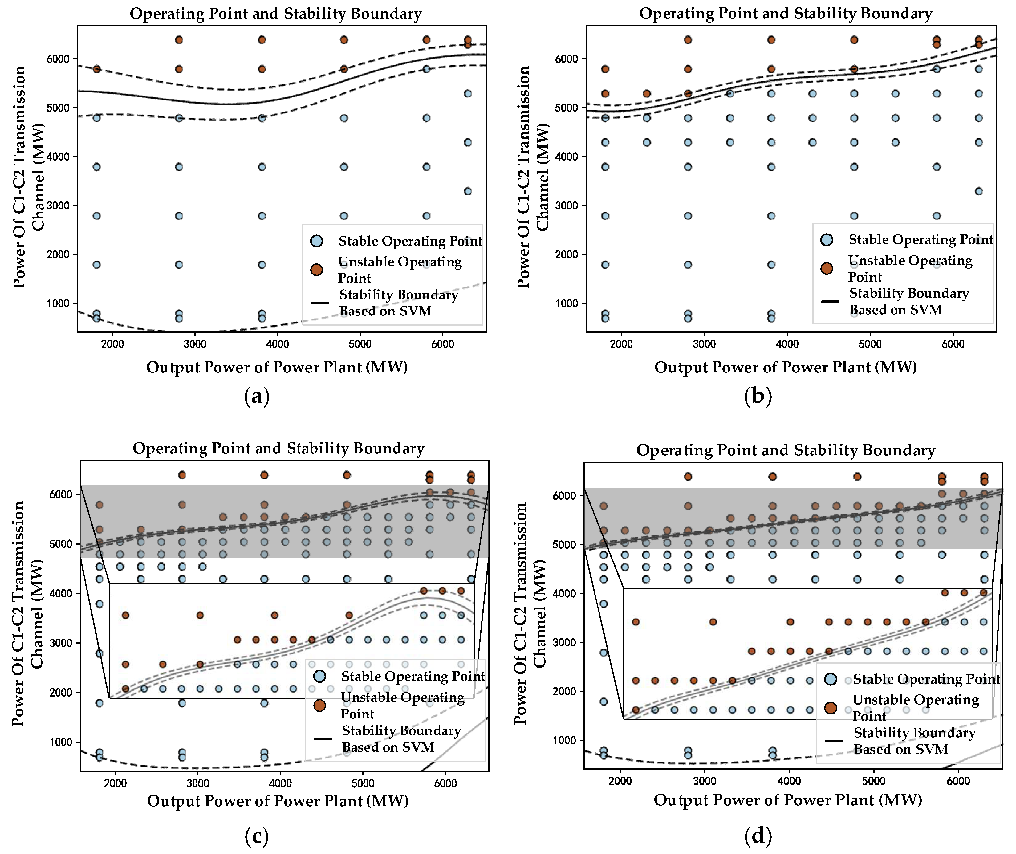
During the four iterations, the distribution of sample points and the evolution of the stability boundary obtained based on the SVM are illustrated in Figure 7 (dotted lines indicate the Support Vector Margins). It can be clearly observed from the figure that the number of samples near the stability boundary has significantly increased while the stability boundary has been continuously refined.

During the four iterations, the re-sampling step size for the second round is V_m,2 = 500, while the step sizes for the third and fourth rounds are V_m,3 = V_m,4 = 250. In practice, the minimum step size for manually adjusting operating points in production processes is typically in the range of 300–500. Therefore, the step size for the third and fourth re-samplings already meets the precision requirements for actual production.

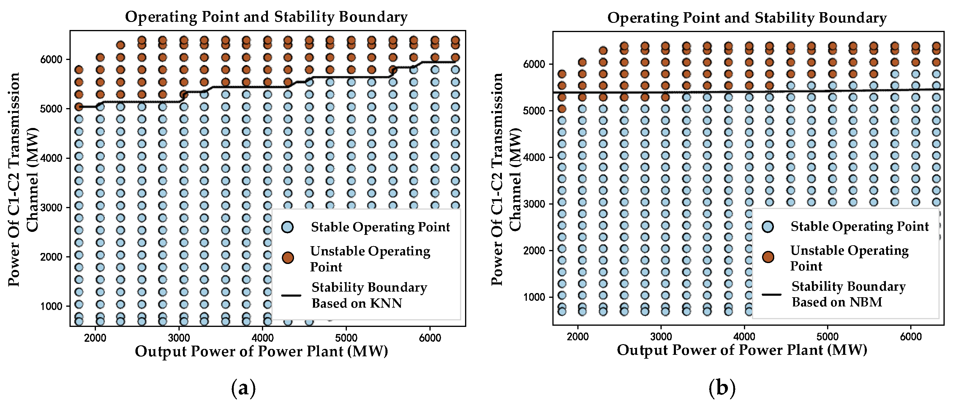
To further substantiate the superiority of the proposed method, we conducted comparative experiments using the K-Nearest Neighbor (KNN) and Naive Bayes Model (NBM), which are commonly employed in existing research. After obtaining a large number of uniformly distributed operating points, we utilized these two methods to classify the operating points and determine the stability boundary. The results are illustrated in Figure 8.

4.3. Performance Analysis

As mentioned above, to calculate the accuracy of the stability boundary obtained by the proposed method in this paper, a two-stage grid scanning method is employed to generate a large number of sample points, thereby obtaining a more precise stability boundary. The distribution of sample points obtained through two-stage grid scanning is shown in Figure 9, where the blue points represent stable points near the stability boundary. In the subsequent ACC calculation, circles with radius R will be drawn centered on these points.

After obtaining a relatively precise stability boundary, the accuracy of the stability boundary obtained in each iteration is calculated using the method introduced in Section 3.4 of this paper. The calculation process of the accuracy for the stability boundary obtained in the fourth iteration is shown in Figure 10 (dotted lines indicate the Support Vector Margins). Here, considering the minimum step size used in practical operations, R is set to 100.

Through the calculation process illustrated in Figure 10, the values of N₁, N₂, N₃, and N₄ for the stability boundary obtained in the fourth iteration can be determined. Similarly, the same procedure is applied to the first three iterations. Considering that the accuracy requirements for stability boundary identification and practical operational constraints (where the 250 MW interval after the fourth iteration falls below the minimum manual adjustment step size), the weighting coefficients are configured as w₁ = 0.8, w₂ = 1, w₃ = 1 and w₄ = 0.6. This configuration applies reduced weights to points beyond the “circle” (w₁, w₄) while maintaining full weights for interior points (w₂, w₃), with a conservative approach assigning higher weights to operating points on the stable side. After that, the accuracy of the stability boundary obtained in each iteration is calculated, as shown in

Table 2. Accuracy of stability boundary obtained from each of the four iterations.

	First Iteration	Second Iteration	Third Iteration	Fourth Iteration
N1	34	5	0	0
N2	11	23	12	19
N3	11	42	54	70
N4	35	21	25	2
ACC	0.7714	0.8967	0.8901	0.9912

.

As shown in Table 2, after four iterations, the accuracy of the obtained stability boundary has reached 99.12%, which meets the requirements of practical production.

Meanwhile, ensuring high accuracy, the time consumed by the proposed method in this paper is significantly less than that of grid scanning, thus greatly improving efficiency. The specific time consumption is shown in

Table 3. Comparison of time spent by the proposed method and grid scanning.

	Proposed Method					Grid Scanning			Time Saved
	First Iteration	Second Iteration	Third Iteration	Fourth Iteration	Subtotal	Stage1	Stage2	Subtotal
operating point generation	46 m 9 s	28 m 20 s	54 m 20 s	9 m 6 s	2 h 17 m 55 s	8 h 12 m 16 s	6 h 22 m 35 s	14 h 34 m 51 s	84.2%
transient simulation	17 m 28 s	14 m 48 s	23 m 42 s	3 m 31 s	59 m 29 s	3 h 8 m 59 s	3 h 30 m2 s	6 h 39 m 1 s	85.1%
total	1 h 3 m 37 s	43 m 8 s	1 h 18 m 2 s	12 m 37 s	3 h 17 m 24 s	11 h 21 m 15 s	9 h 52 m 37 s	21 h 13 m 52 s	84.5%

.

In addition, we have also calculated the ACC of the stability boundaries obtained based on KNN and NBM and recorded the time spent. The comparison with the proposed method in this paper is presented in

Table 4. Comparison of ACC and time spent among the proposed method, KNN, and NBM.

	Proposed Method	KNN	NBM
ACC	0.9912	0.9560	0.7758
time spent	3 h 17 m 24 s	11 h 21 m 15 s	11 h 21 m 15 s *
extra time spent	/	245.11%	245.11%

* Since both the application of KNN and NBM are based on the same set of operating points for classification and stability boundary determination, the time spent for these two methods is identical, corresponding to the time required for generating the operating points and conducting transient simulations.

.

As shown in Table 4, although the stability boundary obtained based on KNN exhibits high accuracy, the time required is significantly greater than that of the proposed method in this paper. Meanwhile, the application of the NBM not only consumes substantial time but also yields a lower accuracy of the stability boundary.

In summary, the method proposed in this paper is capable of rapidly obtaining a stability boundary that meets accuracy requirements based on a small number of sample points. Moreover, it efficiently acquires a large number of stable operating points near the stability boundary under the N-1 fault, providing critical samples for subsequent stability control setting value validation tasks.

5. Conclusions

This paper proposes a method for power system transient stability boundary exploration based on the SVM. By re-sampling around the obtained boundary, stable operating points near the stability boundary under the N-1 fault are acquired, providing critical samples for stability control setting value validation. The case study results indicate that the accuracy of the stability boundary determined using the proposed method reaches 99.12%, which meets the accuracy requirements for practical production. And compared to grid scanning, the proposed method can obtain a large number of stable operating points near the stability boundary in a shorter time (approximately one-seventh of the time spent on grid scanning), thus significantly improving production efficiency. Also, compared with existing methods such as KNN and NBM, the proposed method in this paper not only achieves higher accuracy but also significantly reduces computational time.

For the application of the proposed method in real-world power system operations, we only need to input a small number of operating points, which are uniformly distributed within the operating space (composed of upper and lower limits of power plant outputs and DC transmission power) with stability labels and set the number of iterations N. Relying on the method proposed in this paper, the initial guess stability boundary can be obtained, and critical operating points can be re-sampled. After updating the sample set, the next iteration begins. This process is iterated N times, ultimately obtaining a more precise stability boundary while efficiently acquiring stable operating points near the stability boundary. It is worth noting that the method proposed in this paper is equally applicable to high-dimensional spaces (systems with multiple power plants or DC transmission corridors). In order to present the experimental results in an intuitive manner using planar diagrams, the case studies in this paper employ a two-dimensional simple system.

Considering that the stability operating region (mentioned in Section 2) under the N-2 fault with stability control strategies is not continuous, unstable operating points may also exist within the region, and the proposed scheme in this paper can only provide critical operating points near the boundary for the tasks of stability control setting value validation, how to obtain the unstable points within the region will be the focus of future research.