
The Explanation and Sensitivity of AI Algorithms Supplied with Synthetic Medical Data


Abstract
1. Introduction
- (i)
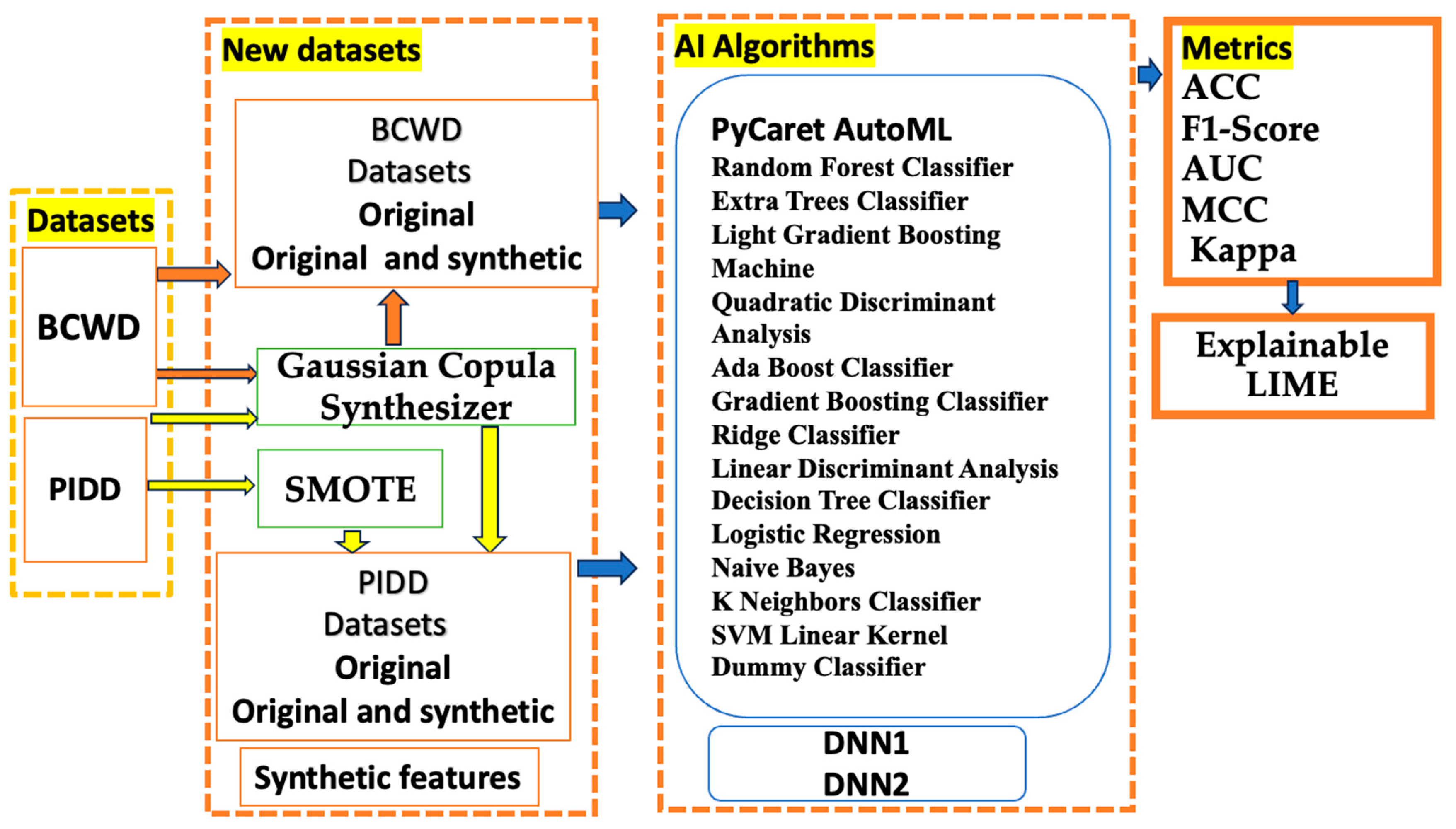
- Proposing the BCWD and PIDD publicly available datasets and building from them the new synthetic dataset (SD) using GCS and SMOTE techniques;
- (ii)
- Synthetic feature creation for the PIDD by applying equal-width and equal-frequency discretization techniques and transforming numerical features into categorical. Combining these synthetic features with the original features improved the classification results.
- (iii)
- PyCaret AutoML and two DNNs were supplied by both PIDD and BCWD datasets, including the original, synthetic, and mixed versions.
- (iv)
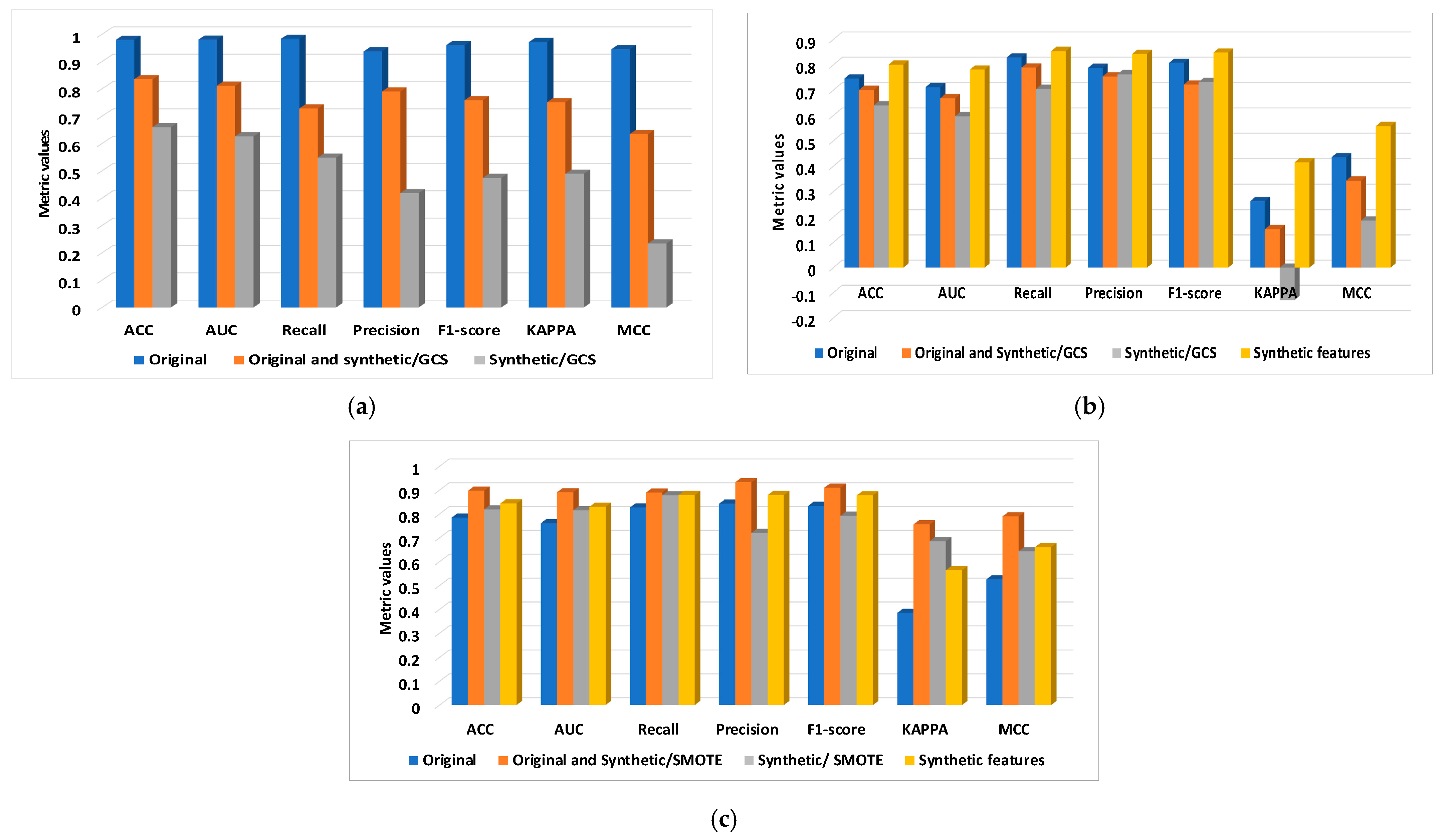
- From the confusion matrix, the ACC, AUC, F1-score, MCC, and Kappa metrics were computed.
- (v)
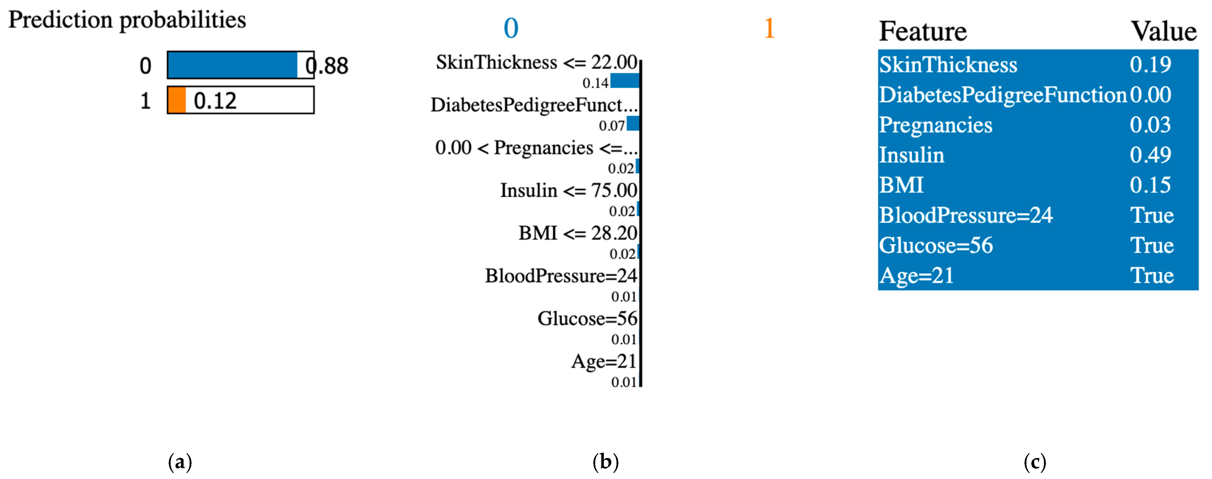
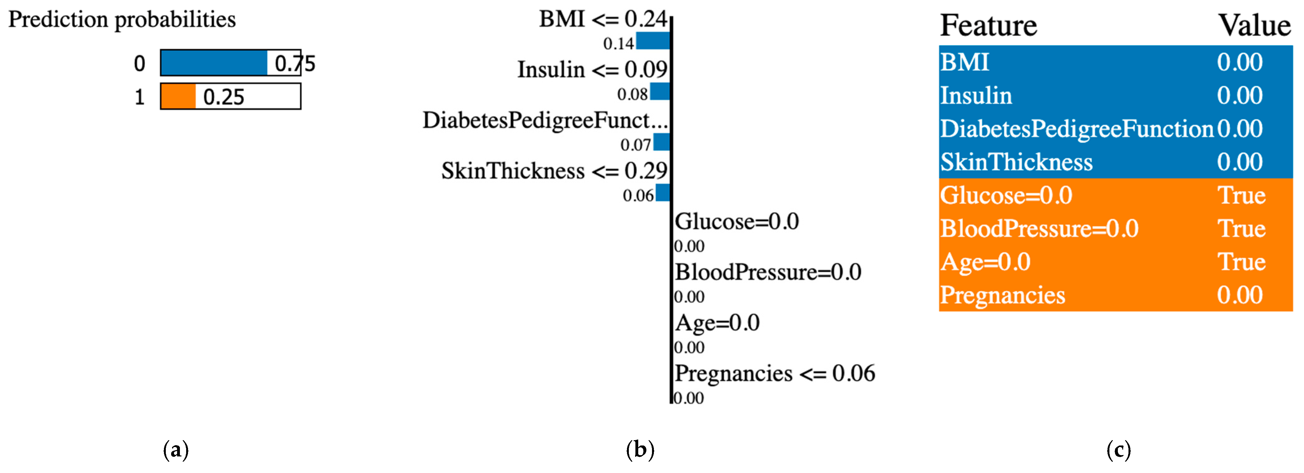
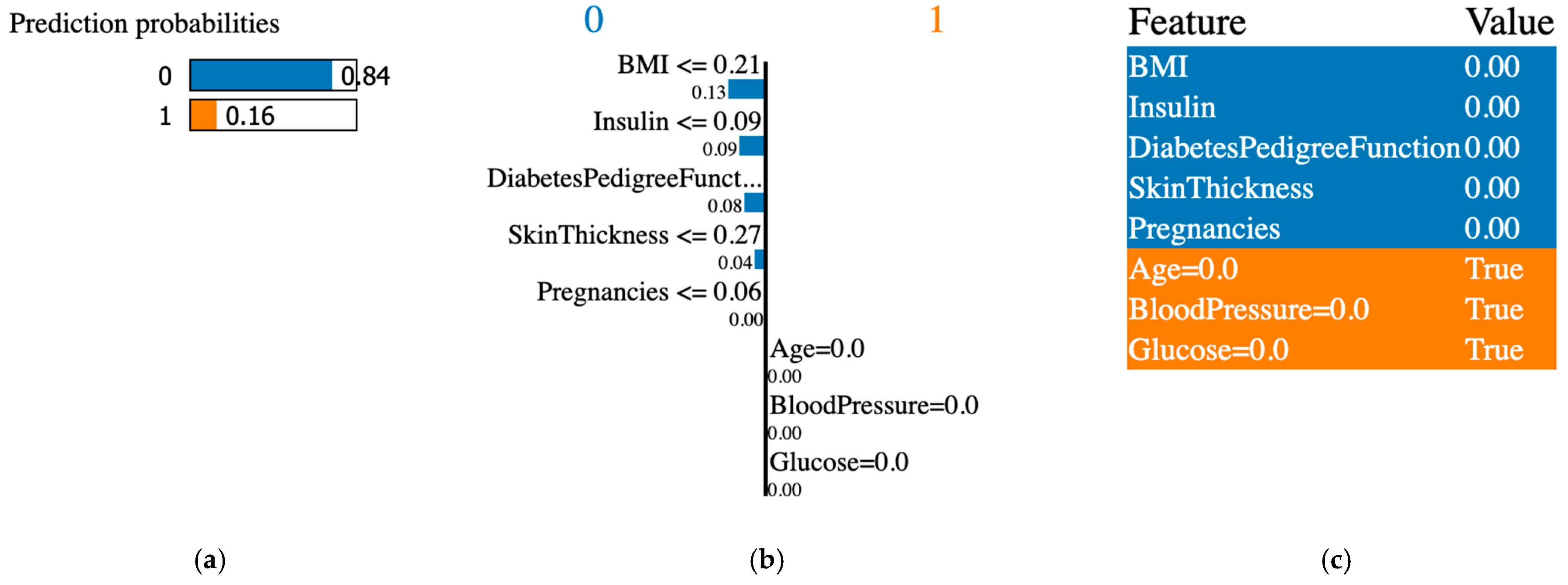
- Explaining the classification with the LIME XAI tool was achieved.
2. Related Works
3. Methodology
4. AI Algorithms
4.1. Gaussian Copula Synthesizer (CGS)
4.2. SMOTE
4.3. Synthetic Features
4.4. AutoML PyCaret
4.5. DNN
4.6. LIME Explainable AI Tool
5. Databases
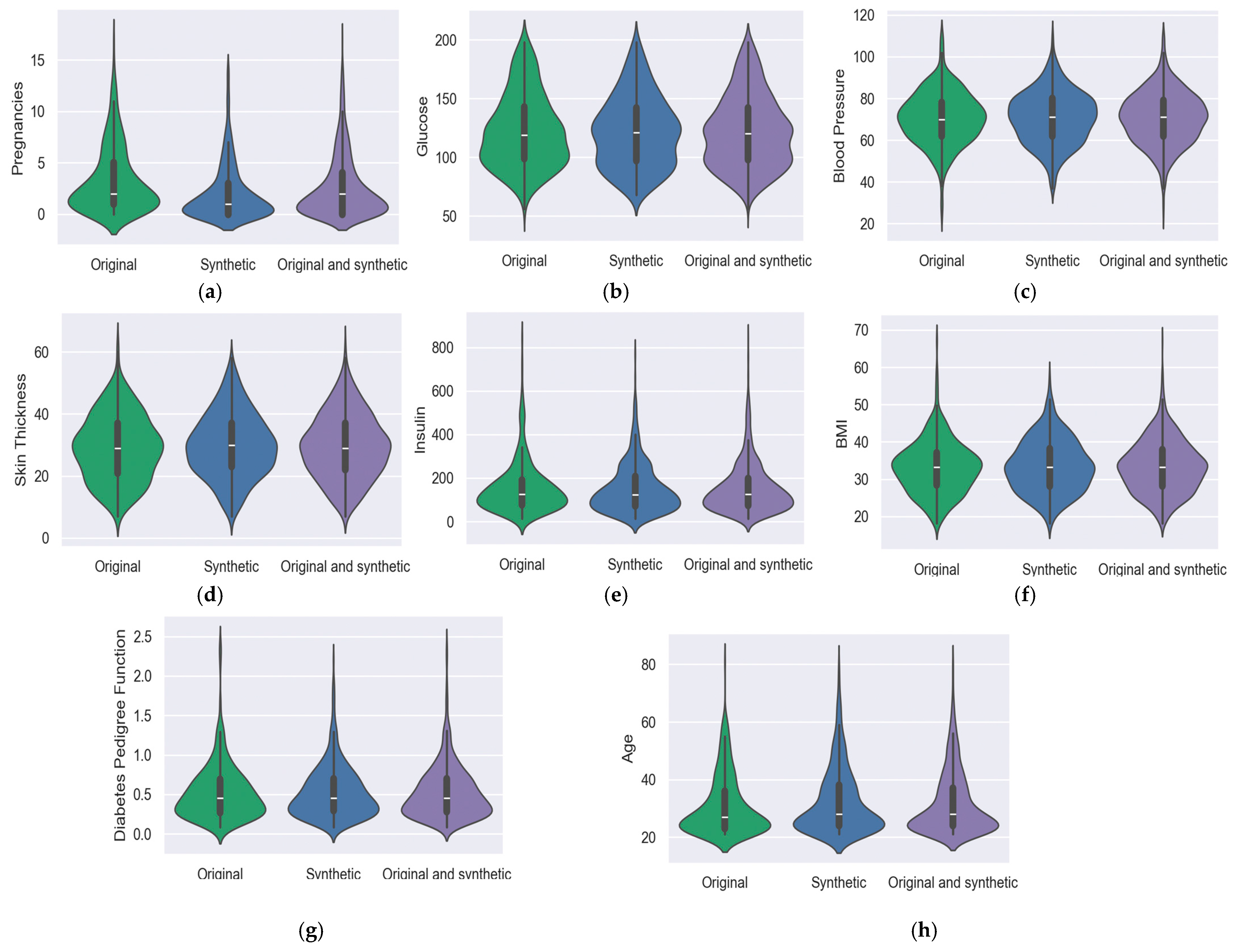
5.1. Pima Indians Diabetes Database (PIDD)
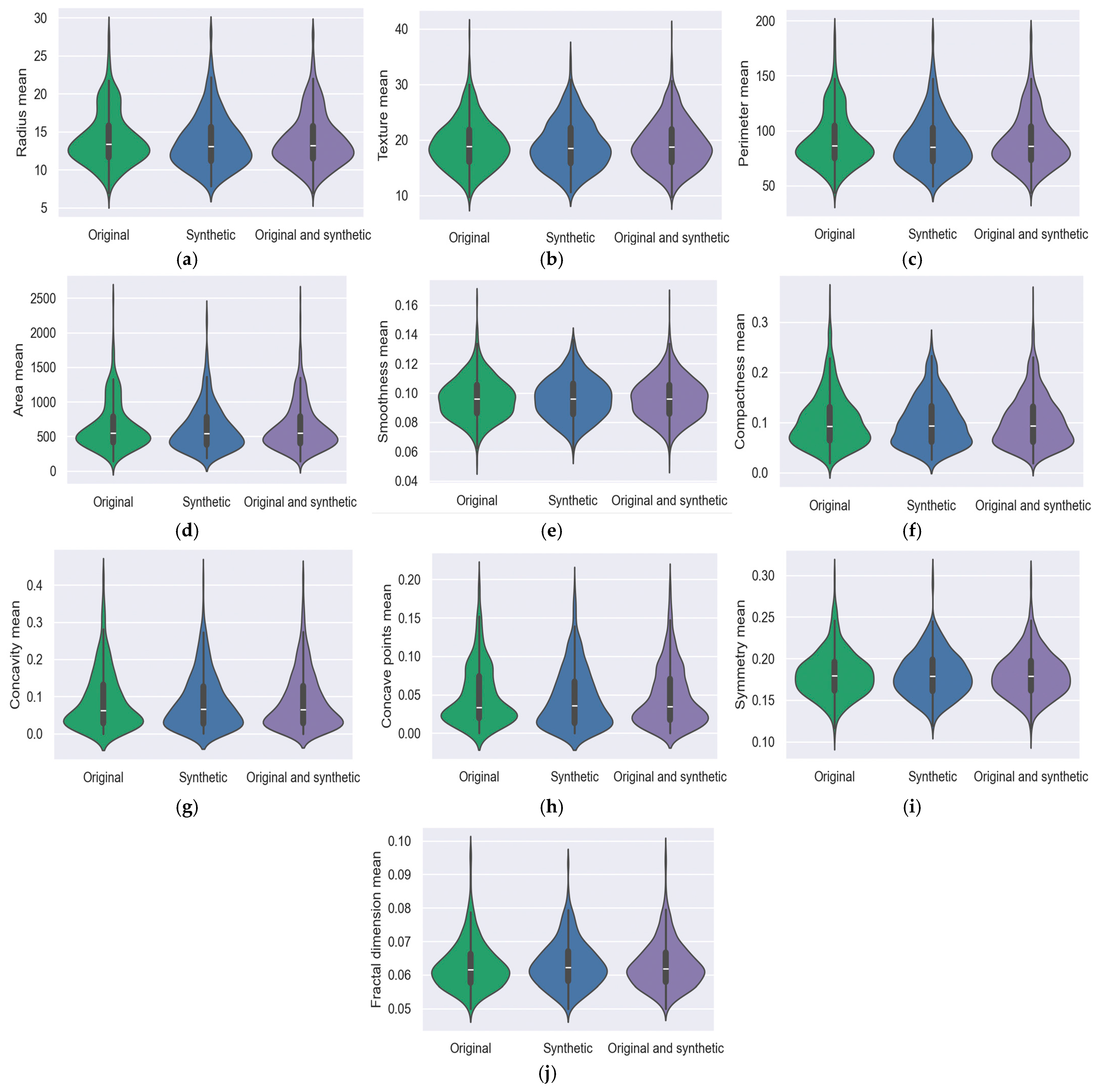
5.2. Breast Cancer Wisconsin Dataset (BCWD)
5.3. Confidence Interval
5.4. Violin Graph
6. Hardware and Software
- NumPy 2.2.1 (https://pypi.org/project/numpy/ (accessed on 22 December 2024));
- Pandas 2.2.3 (https://pandas.pydata.org/docs/whatsnew/index.html (accessed on 22 December 2024));
- TensorFlow 2.17.0 (https://blog.tensorflow.org/2024/07/whats-new-in-tensorflow-217.html (accessed on 22 December 2024));
- Scikit-learn 1.6.1 (https://pypi.org/project/scikit-learn/ (accessed on 11 January 2025));
- PyCaret 3.0.4 (https://pycaret.readthedocs.io/en/stable/installation.html (accessed on 22 December 2024));
- Seaborn 0.13.2 (https://seaborn.pydata.org/installing.html (accessed on 22 December 2024))
- LIME 8.2.2. (https://lib.haxe.org/p/lime/ (accessed on 22 December 2024)).
7. Metrics
8. Results and Discussions
9. Conclusions
Supplementary Materials
Author Contributions
Funding
Data Availability Statement
Conflicts of Interest
References
- An, Q.; Rahman, S.; Zhou, J.; Kang, J.J. A Comprehensive Review on Machine Learning in Healthcare Industry: Classification, Restrictions, Opportunities and Challenges. Sensors 2023, 23, 4178. [Google Scholar] [CrossRef]
- Gonzales, A.; Guruswamy, G.; Smith, S.R. Synthetic Data in Health Care: A Narrative Review. PLoS Digit. Health 2023, 2, e0000082. [Google Scholar] [CrossRef] [PubMed]
- Clemente, F.; Ribeiro, G.M.; Quemy, A.; Santos, M.S.; Pereira, R.C.; Barros, A. ydata-profiling: Accelerating Data-Centric AI with High-Quality Data. Neurocomputing 2023, 554, 126585. [Google Scholar] [CrossRef]
- Patki, N.; Wedge, R.; Veeramachaneni, K. The Synthetic Data Vault. In Proceedings of the 2016 IEEE International Conference on Data Science and Advanced Analytics (DSAA), Montreal, QC, Canada, 17–19 October 2016; pp. 399–410. [Google Scholar] [CrossRef]
- Juneja, T.; Bajaj, S.B.; Sethi, N. Synthetic Time Series Data Generation Using Time GAN with Synthetic and Real-Time Data Analysis. In Proceedings of the Lecture Notes in Electrical Engineering; Springer: Berlin/Heidelberg, Germany, 2023; Volume 1011, pp. 657–667. [Google Scholar] [CrossRef]
- Sei, Y.; Onesimu, J.A.; Ohsuga, A. Machine Learning Model Generation with Copula-Based Synthetic Dataset for Local Differentially Private Numerical Data. IEEE Access 2022, 10, 101656–101671. [Google Scholar] [CrossRef]
- He, X.; Zhao, K.; Chu, X. AutoML: A Survey of the State-of-the-Art. Knowl.-Based Syst. 2021, 212, 106622. [Google Scholar] [CrossRef]
- LeDell, E.; Poirier, S. H2O AutoML: Scalable Automatic Machine Learning. In Proceedings of the 7th ICML AutoML Workshop, Online Event, 18 July 2020; pp. 1–16. Available online: https://www.automl.org/wp-content/uploads/2020/07/AutoML_2020_paper_61.pdf (accessed on 23 October 2024).
- Salih, A.M.; Raisi-Estabragh, Z.; Galazzo, I.B.; Radeva, P.; Petersen, S.E.; Lekadir, K.; Menegaz, G. A Perspective on Explainable Artificial Intelligence Methods: SHAP and LIME. Adv. Intell. Syst. 2024, 7, 2400304. [Google Scholar] [CrossRef]
- Chicco, D.; Tötsch, N.; Jurman, G. The Matthews Correlation Coefficient (MCC) Is More Reliable Than Balanced Accuracy, Bookmaker Informedness, and Markedness in Two-Class Confusion Matrix Evaluation. BioData Min. 2021, 14, 13. [Google Scholar] [CrossRef]
- Tăbăcaru, G.; Moldovanu, S.; Răducan, E.; Barbu, M. A Robust Machine Learning Model for Diabetic Retinopathy Classification. J. Imaging 2023, 10, 8. [Google Scholar] [CrossRef]
- Rujas, M.; Herranz, R.M.G.; Fico, G.; Merino-Barbancho, B. Synthetic Data Generation in Healthcare: A Scoping Review of Reviews on Domains, Motivations, and Future Applications. Int. J. Med. Inform. 2024, 195, 105763. [Google Scholar] [CrossRef]
- Aziz, N.A.; Manzoor, A.; Qureshi, M.D.M.; Qureshi, M.A.; Rashwan, W. Explainable AI in Healthcare: Systematic Review of Clinical Decision Support Systems. medRxiv 2024. [Google Scholar] [CrossRef]
- Hernandez, M.; Epelde, G.; Beristain, A.; Álvarez, R.; Molina, C.; Larrea, X.; Alberdi, A.; Timoleon, M.; Bamidis, P.; Konstantinidis, E. Incorporation of Synthetic Data Generation Techniques within a Controlled Data Processing Workflow in the Health and Wellbeing Domain. Electronics 2022, 11, 812. [Google Scholar] [CrossRef]
- Ibrahim, M.; Al Khalil, Y.; Amirrajab, S.; Suna, C.; Breeuwer, M.; Pluim, J.; Elen, B.; Ertaylan, G.; Dumontier, M. Generative AI for Synthetic Data Across Multiple Medical Modalities: A Systematic Review of Recent Developments and Challenges. Comput. Biol. Med. 2025, 189, 109834. [Google Scholar] [CrossRef] [PubMed]
- Giuffrè, M.; Shung, D.L. Harnessing the Power of Synthetic Data in Healthcare: Innovation, Application, and Privacy. Npj Digit. Med. 2023, 6, 186. [Google Scholar] [CrossRef]
- Chen, R.J.; Lu, M.Y.; Chen, T.Y.; Williamson, D.F.; Mahmood, F. Synthetic Data in Machine Learning for Medicine and Healthcare. Nat. Biomed. Eng. 2021, 5, 493–497. [Google Scholar] [CrossRef]
- Pezoulas, V.C.; Zaridis, D.I.; Mylona, E.; Androutsos, C.; Apostolidis, K.; Tachos, N.S.; Fotiadis, D.I. Synthetic Data Generation Methods in Healthcare: A Review on Open-Source Tools and Methods. Comput. Struct. Biotechnol. J. 2024, 23, 2892–2910. [Google Scholar] [CrossRef]
- Dankar, F.K.; Ibrahim, M. Fake It Till You Make It: Guidelines for Effective Synthetic Data Generation. Appl. Sci. 2021, 11, 2158. [Google Scholar] [CrossRef]
- Wan, C.; Jones, D.T. Protein Function Prediction Is Improved by Creating Synthetic Feature Samples with Generative Adversarial Networks. Nat. Mach. Intell. 2020, 2, 540–550. [Google Scholar] [CrossRef]
- Mahmood, F.; Borders, D.; Chen, R.J.; McKay, G.N.; Saliman, K.; Baras, A. Deep Adversarial Training for Multi-Organ Nuclei Segmentation in Histopathology Images. IEEE Trans. Med. Imaging 2020, 39, 3257–3267. [Google Scholar] [CrossRef]
- Kingma, D.P.; Welling, M. Auto-Encoding Variational Bayes. arXiv 2013, arXiv:1312.6114. [Google Scholar] [CrossRef]
- Khosravi, H.; Das, S.; Al-Mamun, A.; Ahmed, I. Binary Gaussian Copula Synthesis: A Novel Data Augmentation Technique to Advance ML-Based Clinical Decision Support Systems for Early Prediction of Dialysis Among CKD Patients. arXiv 2023, arXiv:2403.00965. [Google Scholar] [CrossRef]
- Torfi, A.; Fox, E.A.; Reddy, C.K. Differentially Private Synthetic Medical Data Generation Using Convolutional GANs. Inf. Sci. 2022, 586, 485–500. [Google Scholar] [CrossRef]
- Rostami, M.; Oussalah, M. A Novel Explainable COVID-19 Diagnosis Method by Integration of Feature Selection with Random Forest. Inform. Med. Unlocked 2022, 30, 100941. [Google Scholar] [CrossRef]
- El-Sofany, H.; Bouallegue, B.; El-Latif, Y.M.A. A Proposed Technique for Predicting Heart Disease Using Machine Learning Algorithms and an Explainable AI Method. Sci. Rep. 2024, 14, 23277. [Google Scholar] [CrossRef]
- Titti, R.R.; Pukkella, S.; Radhika, T.S.L. Augmenting Heart Disease Prediction with Explainable AI: A Study of Classification Models. Comput. Math. Biophys. 2024, 12, 20240004. [Google Scholar] [CrossRef]
- Tasin, I.; Nabil, T.U.; Islam, S.; Khan, R. Diabetes Prediction Using Machine Learning and Explainable AI Techniques. Healthc. Technol. Lett. 2022, 10, 1–10. [Google Scholar] [CrossRef]
- Kibria, H.B.; Nahiduzzaman, M.; Goni, M.O.F.; Ahsan, M.; Haider, J. An Ensemble Approach for the Prediction of Diabetes Mellitus Using a Soft Voting Classifier with an Explainable AI. Sensors 2022, 22, 7268. [Google Scholar] [CrossRef]
- Karimi, D.; Dou, H.; Warfield, S.K.; Gholipour, A. Deep Learning with Noisy Labels: Exploring Techniques and Remedies in Medical Image Analysis. Med. Image Anal. 2020, 65, 101759. [Google Scholar] [CrossRef]
- Chuah, J.; Kruger, U.; Wang, G.; Yan, P.; Hahn, J. Framework for Testing Robustness of Machine Learning-Based Classifiers. J. Pers. Med. 2022, 12, 1314. [Google Scholar] [CrossRef] [PubMed]
- Available online: https://docs.sdv.dev/sdv/single-table-data/modeling/synthesizers/gaussiancopulasynthesizer (accessed on 22 December 2024).
- Available online: https://pycaret.readthedocs.io/en/latest/ (accessed on 22 December 2024).
- Available online: https://lime.readthedocs.io/en/latest/ (accessed on 22 December 2024).
- Hospital Israelita Albert Einstein. Diagnosis of COVID-19 and Its Clinical Spectrum—Ai and Data Science Supporting Clinical Decisions (From 28th Mar to 3st Apr). Available online: https://www.kaggle.com/einsteindata4u/covid19 (accessed on 30 September 2024).
- Available online: https://www.kaggle.com/code/akhiljethwa/heart-failure-classification-knn-decision-tree (accessed on 30 September 2024).
- Chawla, N.V.; Bowyer, K.W.; Hall, L.O.; Kegelmeyer, W.P. SMOTE: Synthetic Minority Over-sampling Technique. J. Artif. Intell. Res. (JAIR) 2002, 16, 321–357. [Google Scholar] [CrossRef]
- Kaur, G.; Reddy, S.; Singh, D.; Sharma, N. A Deep Neural Architecture for Harmonizing 3-D Input Data Analysis and Decision Making in Medical Imaging. arXiv 2023, arXiv:2303.00175. [Google Scholar] [CrossRef]
- Nazir, S.; Kaleem, M. Federated Learning for Medical Image Analysis with Deep Neural Networks. Diagnostics 2023, 13, 1532. [Google Scholar] [CrossRef] [PubMed]
- Sánchez-Gutiérrez, M.E.; González-Pérez, P.P. Multi-Class Classification of Medical Data Based on Neural Network Pruning and Information-Entropy Measures. Entropy 2022, 24, 196. [Google Scholar] [CrossRef] [PubMed]
- Gasmi, A. Deep learning and health informatics for smart monitoring and diagnosis. arXiv 2022, arXiv:2208.03143. [Google Scholar] [CrossRef]
- Street, W.N.; Wolberg, W.H.; Mangasarian, O.L. Nuclear feature extraction for breast tumor diagnosis. In Proceedings of the IS&T/SPIE 1993 International Symposium on Electronic Imaging: Science and Technology, San Jose, CA, USA, 31 January–5 February 1993; Volume 1905, pp. 861–870. [Google Scholar] [CrossRef]
- Sellat, Q.; Bisoy, S.K.; Priyadarshini, R. Chapter 10—Semantic Segmentation for Self-Driving Cars Using Deep Learning: A Survey. In Cognitive Big Data Intelligence with a Metaheuristic Approach; Mishra, S., Tripathy, H.K., Mallick, P.K., Sangaiah, A.K., Chae, G.-S., Eds.; Academic Press: Cambridge, MA, USA, 2022; pp. 211–238. [Google Scholar] [CrossRef]
- Morabito, F.C.; Kozma, R.; Alippi, C.; Choe, Y. Advances in AI, neural networks, and brain computing: An introduction. In Artificial Intelligence in the Age of Neural Networks and Brain Computing; Academic Press: Cambridge, MA, USA, 2024; pp. 1–8. [Google Scholar] [CrossRef]
- Sadiq, I.Z.; Usman, A.; Muhammad, A.; Ahmad, K.H. Sample size calculation in biomedical, clinical and biological sciences research. J. Umm Al-Qura Univ. Appl. Sci. 2024, 11, 133–141. [Google Scholar] [CrossRef]


| Data Type | Classifier | |
|---|---|---|
| BCWD | Original | RandomForestClassifier (criterion = ‘gini’, max_features = ‘sqrt’, n_estimators = 100) |
| Original and synthetic/GCS | RandomForestClassifier (criterion = ‘gini’, max_features = ‘sqrt’, n_estimators = 100) | |
| Synthetic/GCS | LinearDiscriminantAnalysis (solver = ‘svd’, tol = 0.0001) | |
| PIDD | Original | GradientBoostingClassifier (criterion = ‘friedman’ learning_rate = 0.1, n_estimators= 100) |
| Original and synthetic/GCS | LogisticRegression (intercept_scaling = 1, max_iter = 1000, multi_class = ‘auto’, penalty = ‘l2’, | |
| Synthetic/GCS | GaussianNB (priors = None, var_smoothing = 1 × 10⁻⁹) | |
| Synthetic features/GCS | AdaBoostClassifier (algorithm = ‘SAMME.R’, learning_rate = 1.0, n_estimators = 50, random_state = 123) | |
| Original and synthetic/SMOTE | ExtraTreesClassifier (criterion = ‘gini’, n_estimators = 100) | |
| Synthetic/ SMOTE | RandomForestClassifier (criterion = ‘gini’, max_features = ‘sqrt’, n_estimators = 100) |
| Datasets/DNN | New Datasets | ACC | AUC | Recall | Precision | F1-Score | KAPPA | MCC |
|---|---|---|---|---|---|---|---|---|
| BCWD/ DNN1 | Original | 0.979 | 0.980 | 0.983 | 0.937 | 0.960 | 0.971 | 0.945 |
| Original and synthetic/GCS | 0.835 | 0.811 | 0.728 | 0.790 | 0.758 | 0.751 | 0.634 | |
| Synthetic/GCS | 0.660 | 0.626 | 0.548 | 0.418 | 0.474 | 0.489 | 0.234 | |
| PIDD/ DNN1 | Original | 0.746 | 0.712 | 0.829 | 0.788 | 0.808 | 0.263 | 0.435 |
| Original and synthetic/GCS | 0.701 | 0.668 | 0.789 | 0.754 | 0.722 | 0.152 | 0.343 | |
| Synthetic/GCS | 0.640 | 0.597 | 0.705 | 0.763 | 0.732 | −0.129 | 0.186 | |
| Synthetic features | 0.801 | 0.781 | 0.854 | 0.843 | 0.848 | 0.415 | 0.558 | |
| PIDD/ DNN2 | Original | 0.785 | 0.761 | 0.827 | 0.843 | 0.834 | 0.385 | 0.526 |
| Original and synthetic/SMOTE | 0.897 | 0.891 | 0.890 | 0.933 | 0.910 | 0.756 | 0.790 | |
| Synthetic/SMOTE | 0.819 | 0.815 | 0.878 | 0.720 | 0.792 | 0.686 | 0.644 | |
| Synthetic features | 0.844 | 0.830 | 0.879 | 0.879 | 0.878 | 0.564 | 0.661 |
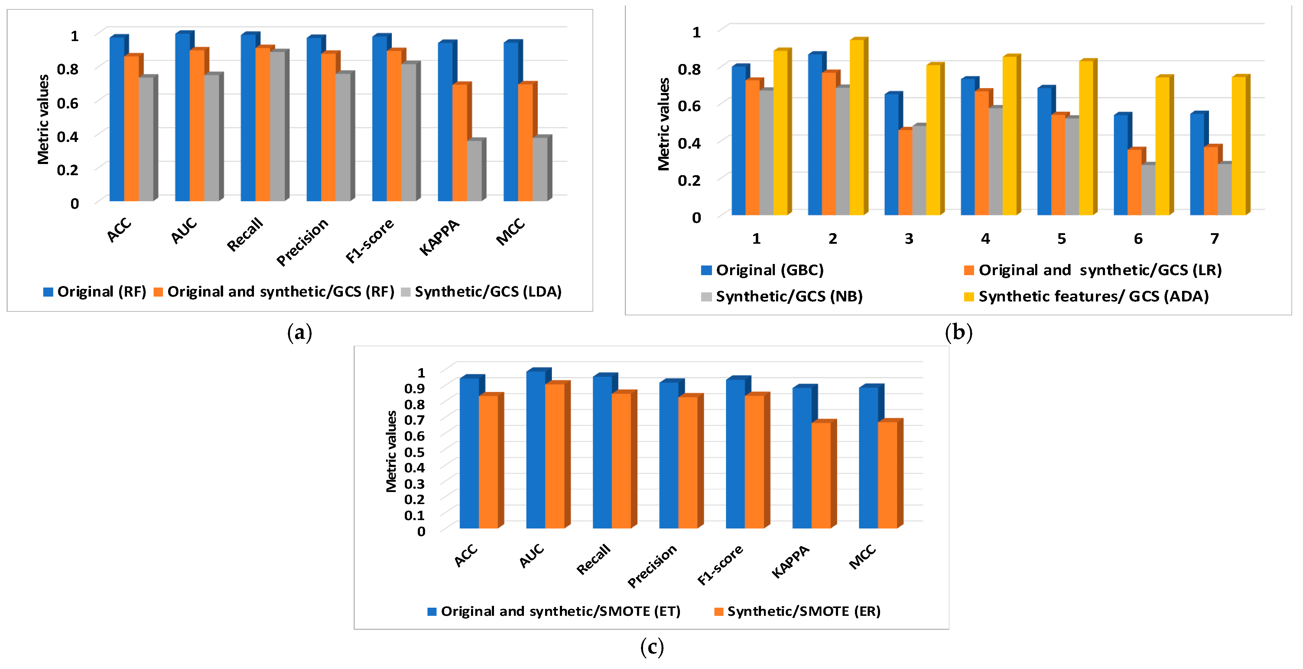
| Dataset | New Datasets | Classifiers | ACC | AUC | Recall | Precision | F1-Score | KAPPA | MCC |
|---|---|---|---|---|---|---|---|---|---|
| BCWD | Original | RF | 0.972 | 0.995 | 0.988 | 0.970 | 0.978 | 0.940 | 0.942 |
| Original and synthetic/GCS | RF | 0.860 | 0.896 | 0.910 | 0.876 | 0.892 | 0.691 | 0.694 | |
| Synthetic/GCS | LDA | 0.734 | 0.749 | 0.886 | 0.757 | 0.814 | 0.358 | 0.376 | |
| PIDD | Original | GBC | 0.799 | 0.865 | 0.649 | 0.731 | 0.682 | 0.537 | 0.544 |
| Original and synthetic/GCS | LR | 0.724 | 0.766 | 0.457 | 0.665 | 0.538 | 0.351 | 0.366 | |
| Synthetic/GCS | NB | 0.669 | 0.684 | 0.479 | 0.574 | 0.519 | 0.269 | 0.274 | |
| Synthetic features/GCS | ADA | 0.884 | 0.942 | 0.807 | 0.852 | 0.828 | 0.741 | 0.743 | |
| Original and synthetic/SMOTE | ET | 0.942 | 0.985 | 0.953 | 0.916 | 0.934 | 0.882 | 0.884 | |
| Synthetic/SMOTE | FR | 0.831 | 0.905 | 0.846 | 0.824 | 0.833 | 0.662 | 0.667 |
| Datasets/DNN | New Datasets | Training Time (s) | Test Time (s) | Training Accuracy |
|---|---|---|---|---|
| BCWD/ DNN1 | Original | 2.772 | 0.019 | 0.998 |
| Original and synthetic/GCS | 3.002 | 0.022 | 0.932 | |
| Synthetic/GCS | 2.654 | 0.019 | 0.779 | |
| PIDD/ DNN1 | Original | 2.935 | 0.031 | 0.899 |
| Original and synthetic/GCS | 3.623 | 0.071 | 0.798 | |
| Synthetic/GCS | 2.336 | 0.015 | 0.730 | |
| Synthetic features | 3.441 | 0.009 | 0.908 | |
| PIDD/ DNN2 | Original | 3.412 | 0.017 | 0.883 |
| Original and synthetic/SMOTE | 4.756 | 0.019 | 0965 | |
| Synthetic/SMOTE | 3.443 | 0.009 | 0.969 | |
| Synthetic features | 2.312 | 0.006 | 0.905 |
| Datasets/PyCaret | New Datasets | Test Time (s) |
|---|---|---|
| BCWD | Original | 0.211 |
| Original and synthetic/GCS | 0.311 | |
| Synthetic/GCS | 0.291 | |
| PIDD | Original | 0.117 |
| Original and synthetic/GCS | 0.223 | |
| Synthetic/GCS | 0.109 | |
| Synthetic features/GCS | 0.213 | |
| Original and synthetic/SMOTE | 0.338 | |
| Synthetic/SMOTE | 0.213 |
| References | ML | Dataset | XAI | Weakness |
|---|---|---|---|---|
| Rostami et al., 2022 [25] | - | COVID-19 dataset [37] | A new Explainable Random Forest called Feature Selection with Explainable Random Forest (FSXRF) | A lack of synthetic data integration, focusing mainly on feature selection and explainability |
| El-Sofany et al., 2024 [26] | Support Vector Machines (SVM), XGBoost, Bagging, Decision Trees (DT), and Random Forests (RF). | CHDD dataset with 303 samples and a private dataset with 200 samples for heart disease prediction | SHAP | The models are evaluated only on real data |
| Titti et al., 2024 [27] | Logistic Regression, K-Nearest Neighbors (KNN), Decision Tree (DT), XGBoost, and CatBoost | Heart disease dataset from Kaggle [38] | Conformalized Quantile Regression and Explainable Boosting Classifier | Not examined whether the models maintain their performance or exhibit vulnerabilities when exposed to synthetic data |
| Tasin et al., 2022 [28]. | Decision Tree, K-Nearest Neighbors (KNN), Random Forest, Support Vector Machines, Logistic Regression, AdaBoost, XGBoost, Voting Classifier, and Bagging | Pima Indian Diabetes Dataset and 203 individuals from a local textile factory in Bangladesh | LIME and SHAP | Not investigated how machine learning models perform with synthetic data |
| Kibria et al., 2022 [29] | Artificial Neural Network (ANN), Random Forest (RF), Support Vector Machine (SVM), Logistic Regression (LR), AdaBoost, and XGBoost | Pima Indian Diabetes Dataset | SHAP | Did not consider synthetic data |
Disclaimer/Publisher’s Note: The statements, opinions and data contained in all publications are solely those of the individual author(s) and contributor(s) and not of MDPI and/or the editor(s). MDPI and/or the editor(s) disclaim responsibility for any injury to people or property resulting from any ideas, methods, instructions or products referred to in the content. |
© 2025 by the authors. Licensee MDPI, Basel, Switzerland. This article is an open access article distributed under the terms and conditions of the Creative Commons Attribution (CC BY) license (https://creativecommons.org/licenses/by/4.0/).
Share and Cite
Munteanu, D.; Moldovanu, S.; Miron, M. The Explanation and Sensitivity of AI Algorithms Supplied with Synthetic Medical Data. Electronics 2025, 14, 1270. https://doi.org/10.3390/electronics14071270
Munteanu D, Moldovanu S, Miron M. The Explanation and Sensitivity of AI Algorithms Supplied with Synthetic Medical Data. Electronics. 2025; 14(7):1270. https://doi.org/10.3390/electronics14071270
Chicago/Turabian StyleMunteanu, Dan, Simona Moldovanu, and Mihaela Miron. 2025. "The Explanation and Sensitivity of AI Algorithms Supplied with Synthetic Medical Data" Electronics 14, no. 7: 1270. https://doi.org/10.3390/electronics14071270
APA StyleMunteanu, D., Moldovanu, S., & Miron, M. (2025). The Explanation and Sensitivity of AI Algorithms Supplied with Synthetic Medical Data. Electronics, 14(7), 1270. https://doi.org/10.3390/electronics14071270