Article

Three-Dimensional Hybrid Finite Element–Boundary Element Analysis of Linear Induction Machines

1
Department of Electronic & Communication Engineering, Uruk University, Baghdad 10001, Iraq
2
Department of Electronics Engineering Technology, Sinclair College, Dayton, OH 45402, USA
*
Author to whom correspondence should be addressed.
Electronics 2025, 14(7), 1261; https://doi.org/10.3390/electronics14071261
Submission received: 16 February 2025 / Revised: 16 March 2025 / Accepted: 21 March 2025 / Published: 23 March 2025
(This article belongs to the Section Electrical and Autonomous Vehicles)

Abstract

:
A three-dimensional model of a three-phase linear induction motor (LIM) is analyzed by using hybrid finite element–boundary element (FEM-BEM) analysis. Two models with aluminum rotors are considered, one with back iron and the other without back iron. The outer boundary is chosen arbitrarily in free space to enclose the motor. The problem domain is divided into rectangular brick elements. The FEM is applied for the interior region, and the BEM is applied for the outer surface. The iron parts can be simulated either as constant permeability regions or regions with the actual magnetization B-H curve. The electromagnetic field problem is solved in terms of the magnetic vector potential. Performance parameters such as propulsion force, levitation force, and dissipated power are then obtained. A comparison of the results with the available measurements from cited references shows agreement within 4–5% for the model without back iron and 9–14% for the model with back iron. It also shows the significant impact of the hybrid FEM-BEM in comparison with the FEM.

1. Introduction

The linear induction motor (LIM) is an electric machine whose topology is such that the electromotive force produces linear motion directly; this is in contrast to rotary machines, where linear motion is obtained by mechanical conversion. The rapid development in LIMs and the wide applications for such machines in transportation have led to the use of different numerical and analytical techniques to solve the associated magnetic field problem, where the obtained results are used to compute the machine performance parameters. Many researchers have worked on numerical techniques in 2D and 3D models using mainly the FEM [1,2,3,4,5]. In [1], periodic boundary conditions are applied together with using edge elements to account for an infinite boundary in which a large number of elements are used. The paper focuses mainly on thrust as an output performance parameter and ignores other performance calculations. Ref. [2] focuses on the design of a special type of LIM, in which a single-sided secondary with skewed bars is used to account for end effects in high-speed machines. The analytical design method is compared with 2D and 3D FEM codes. In [3], a 2D hybrid FEM-BEM method was adopted for the analysis of sheet rotor single-sided LIMs. The analysis did not take into account transverse edge effects and no model of a rotor with a back iron was analyzed. Ref. [4] developed a design technique for the secondary member of a double-sided LIM to account for longitudinal effects by adopting the concept of the ratio of ladder width to slot width, and then the results were compared with FEM code. This analytical technique did not take transverse edge effects into consideration, which can be predicted through measurements only. In [5], an analytical model of SLIMs with asymmetry was presented. The transverse force, air-gap flux density, and eddy current in the secondary were predicted and validated by measurement on a SLIM with transverse asymmetry when two types of secondary (flat and cap) were applied. This analytical solution did not cover every performance calculation accurately. Another SLIM was studied in [6] to produce an equivalent circuit based on the winding method. Again, as an analytical method, the equivalent circuit suffers from shortcomings such as longitudinal and transverse edge effects, leading researchers to try to find correction factors to account for these shortcomings. Ref. [7] proposed an analytical method using a transverse edge coefficient in high-temperature superconducting LIM and compared that with FEM code. It was found that this coefficient is very sensitive to many factors such as supply frequency, mechanical clearance, and core width. The equivalent circuit method for SLIM was adopted in [8,9] with correction factors to account for longitudinal, transverse, asymmetry, and skin effects. The space harmonic method was proposed in [10] to calculate efficiency and ohmic losses in the secondary, which was backed by iron. The study, however, did not include a case where the rotor was not a composite material. Ref. [11] focuses on reducing the transverse forces produced by using a ladder-slit secondary, which is a special type of LIM using 3D FEM. In [12], a finite set model was introduced to maximize the thrust and reduce thrust ripple; this is a design criterion to control the propulsion force. Ref. [13] deals with special transport systems, working in the conditions of hermetic protective chambers with an aggressive radioactive environment in order to calculate propulsion forces through an analytical method. In [14], transverse edge effects were reduced in SLIM using 3D FEM with an optimization method but the analysis was restricted to low-speed LIMs. Ref. [15] adopted another design criterion to optimize the efficiency of LIMs by utilizing end effects and a large air gap.
Since 3D models take both the longitudinal and transverse end effects into account, while in 2D models, only the longitudinal end effects are considered, the main objective of this paper is to present a three-dimensional hybrid FEM-BEM analysis of the LIM performance of two LIM models, one with backing iron and one without it, as a fast and efficient tool. The suggested technique has the following advantages:
(1)
It considers the real shape of the machine and takes into consideration the end effects both in the longitudinal and transverse directions.
(2)
The actual stator slots housing the three-phase coils are represented in the models rather than the familiarly used infinitesimally current sheet to simulate the stator current excitation.
(3)
Iron parts can be simulated either as constant permeability regions or represented by their actual nonlinear B-H curve.
(4)
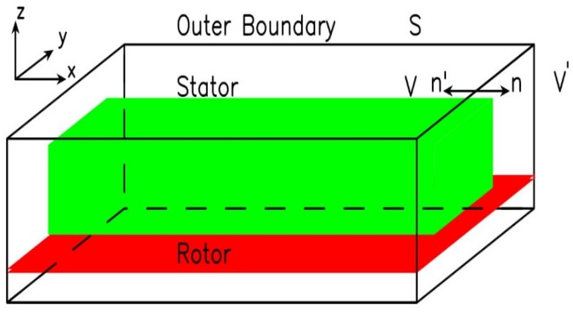
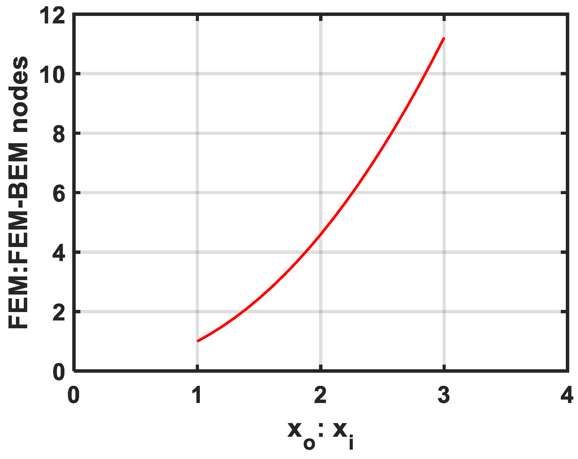
It is not necessary to have a far boundary as in the conventional FEM. Instead of that, an arbitrary boundary is chosen at any distance close to the machine ends, which leads to minimization of the dimensions of the problem domain and the associated computer storage and computation time, while in the FEM, the same accuracy can be obtained by choosing a farther outer boundary from the machine ends.
As a second objective, this adopted numerical technique serves as an effective tool for the machine designer to select the suitable machine parameters for their design requirements and find the effects on performance parameters at different design stages, such as
i.
The effect of changing the frequency or slip.
ii.
The effect of changing the coils’ distribution and the magnetic poles’ configuration.
iii.
Evaluation of the effect of using back iron in comparison with the case of using sheet rotor only.

2. Mathematical Model

Figure 1 shows the three-dimensional model considered in this paper. The model consists of a short stator backed by iron with three-phase coils distributed in the slots, and the rotor is represented by a long aluminum sheet. An outer surface boundary S is arbitrarily chosen to enclose the machine, represented by the interior region V. The FEM is applied for the interior region V and the BEM method is applied on the surface S. Cartesian coordinates are adopted, where the coils’ exciting currents, and therefore the current density J and the magnetic vector potential A, are in the positive y direction. In the FEM solution, Dirichlet boundary conditions are applied to all boundary surfaces since FEM assumes infinite boundaries sufficiently far from the motor outer dimensions and at which the magnetic vector potential A reduces to zero, which dictates the use of a higher number of nodes. This means more computer storage is required and increases the execution time. Meanwhile, in the hybrid FEM-BEM solution, the magnetic vector potential is left free to be evaluated at the nodes located on the boundary surface chosen arbitrarily near the motor outer dimensions throughout the boundary element formulation. The nodes at which the rotor meets the boundaries along the x direction are excluded from the boundary element formulation, and Neumann boundary conditions are applied to these nodes in order to ensure periodic boundary conditions. The propulsion force obtained is in the longitudinal x direction, and the levitation force is in the vertical z direction. Using Maxwell’s equations, the governing partial differential equation in terms of A is
× 1 μ × A = J . J e = 0
where µ is the permeability, Je represents the current density in the rotor conductor elements, and in the stator coil elements, the current density is denoted by J0, where
J e = σ ( A t + v × B φ )
and where σ is the rotor conductivity, v is the rotor velocity, B is the magnetic flux density, and φ is a scalar potential.
The term ∇φ in (2) is added to ensure that no current can enter or leave the conductor surface [16]. To reduce the number of variables, φ can be removed by taking the divergence of (2) and adopting the Coulomb gauge (∇. A = 0) [17], and φ can be expressed in terms of A (see Appendix A) as
φ = ( v . A )
then, we have
v × × A φ = ( v . ) A
Substituting (3) into (1) and (2), assuming all parameters vary sinusoidally with time, and adopting complex notation to replace the time derivative results in
× ( 1 μ × A ) + σ [ j ω A + ( v . ) A ] = J 0
where ω is the angular frequency.
Applying the Galerkin weighted residual method [17] to (4) results in
V N i [ × 1 μ × A + j ω σ A + σ ( v . ) A ] d V = V N i J 0 d V
Using Gauss’s theorem, (5) can be written as
V [ N i × 1 μ × A + j ω σ N i A + σ N i ( v . ) A ] d V S N i ( n × 1 μ × A ) d S = V N i J 0 d V
The system of equations in (6) represents the three components of the magnetic vector potential A and it is the governing equation to be discretized to find the numerical solution.

3. FEM Formulation

The interior problem domain is discretized into brick elements of eight nodes each. At any point within the brick element, the magnetic vector potential A is given by
A = i = 1 8 N i A i
where Ni is a continuous shape function throughout the element and has the value
N i = 1      at   node   i
N i = 0      at   any   other   node  
The shape function guarantees the continuity of magnetic vector potential along element boundaries.
Taking into consideration that the impressed current in the coils of the considered models is assumed in the transverse (y) direction, while it is assumed in the x direction in the overhang, and the rotor speed has only one component, which is in the x direction, the scalar equations for the x, y, and z components of the magnetic vector potential are obtained from (6).
The discretized form of each of these components leads to the following coefficients of the stiffness matrix, i.e., for the y component, the coefficients are
S i j = V 1 μ ( N i x . N j x + N i z . N j z ) d x d y d z + V j ω σ N i N j d x d y d z + V σ v x N i N j x d x d y d z
T i = V N i J 0 d x d y d z
D i k = 1 μ 0 s N i d S k
where Ti has values only for coil elements. Dik has values only for the boundary nodes. Derivations for the x and z components of A can be obtained in a similar way.

4. BEM Formulation

The surface S enclosing the problem domain is taken arbitrary in space; therefore,
2 A = 0
To find a solution to (11), Green’s function is introduced [17], such that
2 G = δ ( x x 0 ) . δ ( y y 0 ) . δ ( z z 0 )
where δ is the Dirac delta function satisfying the following condition:
A ( x 0 , y 0 , z 0 ) δ ( x x 0 ) δ ( y y 0 ) δ ( z z 0 ) d x d y d z = A ( x 0 , y 0 , z 0 )
Green’s function in three dimensions is given by
G = 1 4 π r = 1 4 π ( x x 0 ) 2 + ( y y 0 ) 2 + ( z z 0 ) 2
where (x0, y0, z0) represents the source point and (x, y, z) represents the observation point.
Multiplying (11) by G and (12) by A, subtracting the resulting equations, and integrating over the exterior region results in
V ( G 2 A A 2 G ) d V = V A . δ ( x x 0 ) . δ ( y y 0 ) . δ ( z z 0 ) d x d y d z
Applying Green’s first identity for any point in the exterior region leads to
S ( G A n A G n ) d S = A ( x 0 , y 0 , z 0 )
where n’ is the unit inward normal vector to the surface S, as shown in Figure 1. The surface S is discretized into two-dimensional rectangular elements. The corner nodes of the surface elements are the same FEM nodes that are lying on the surface.
At any point within the surface elements, A is given by
A = i = 1 4 M i A i
A n = i = 1 4 M i n A i
where Mi is the shape function with a value of 1 at node i and 0 at other nodes. Assuming constant surface elements and taking the values of A and A n at the element center each as a representative for the whole element result in
A ( B ) = 1 4 i = 1 4 A i ( F )
When applying (16) to the point (x0, y0, z0), a problem of singularity appears since r = 0.
To avoid singularity, a small hemisphere of radius rs centered at (x0, y0, z0) is considered [18,19], as shown in Figure 2. The surface integral in (16) is split into two parts:
S ( G A n A G n ) d S = S S 1 ( G A n A G n ) d S + S 1 ( G A n A G n ) d S
where the first term in the right-hand side of (20) represents the integration over the surface S minus the surface of the small hemisphere. Integration over S1 is obtained by noting that
G = 1 4 π r s   and   G n = G r s = 1 4 π r s 2   and S 1 ( G A n A G n ) d S = S 1 G A n d S S 1 A G n d S
Since A and its normal derivative are assumed constant over the surface S1, then
S 1 ( G A n A G n ) d S = A n 0 π 0 π 1 4 π r s r s 2 sin θ d θ d ϕ + A . 0 π 0 π 1 4 π r s 2 r s 2 sin θ d θ d ϕ
As rs tends to zero, the first term of the right-hand side of (21) tends to zero; then,
S 1 ( G A n A G n ) d S = 1 2 A ( x 0 , y 0 , z 0 )
Substituting (22) into (16) results in
S S 1 ( G A n A G n ) d S = 1 2 A ( x 0 , y 0 , z 0 )
For the discretization of (23), we set the sampling points at the center of each surface element. Assuming A and  A n are uniform across each element, then (23) can be written in matrix form as
[ F ] { q } C ( B ) [ H ] { A } C ( B ) = { 0 }
where the superscript B stands for BEM formulation, q = A n . The elements of matrices [F] and [H] are deduced from (16), taking into consideration the singularity treatment as given below:
F i j = S j G i j d S = G i j Δ S j     for   i     j   F i j = S i G i i d S = G i i Δ S i     for   i   =   j  
H i j = S j G i j n d S     for   i     j   H i j = 1 2     for   i   =   j  
where Si and Sj denote the surface area of the i-th and j-th boundary elements, respectively. Gij and G i j n denote the values of G and its normal derivative at the j-th element caused by a source at the i-th element, which are computed using (14). G n takes the values of G x , G y , or G z according to the location of the j-th element on the surface.
The integrals in (25) and (26) are obtained numerically. Each surface element is divided into a number of sub-elements. The sub-element containing the singularity is excluded since it has been computed separately in Equation (22). The integrals are approximated by the following summations, where Wm and Wn are the length and width of the mn-th sub-element, respectively.
S i S 1 G i i n d S = n = 1 k m = 1 k G m n n W m W n S i S 1 G i j d S = n = 1 k m = 1 k G m n W m W n
Different values of rs and k have been tried, and it was found that the accuracy of computing (27) was better than 1% for rs less than 1% of the element dimensions and k greater than 100.
The outer boundary is assumed to move with the stator at the same velocity; hence, the relative motion between them is zero. Taking into consideration an infinitely long rotor, the BEM formulation is not affected by the stator motion.

5. Coupling of the BEM with the FEM
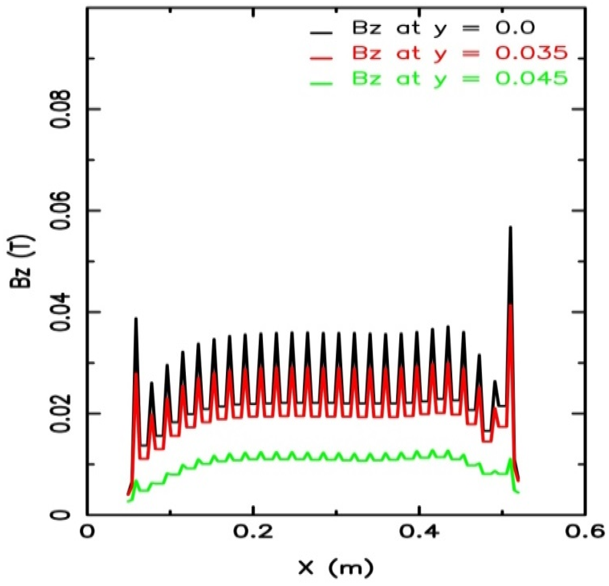
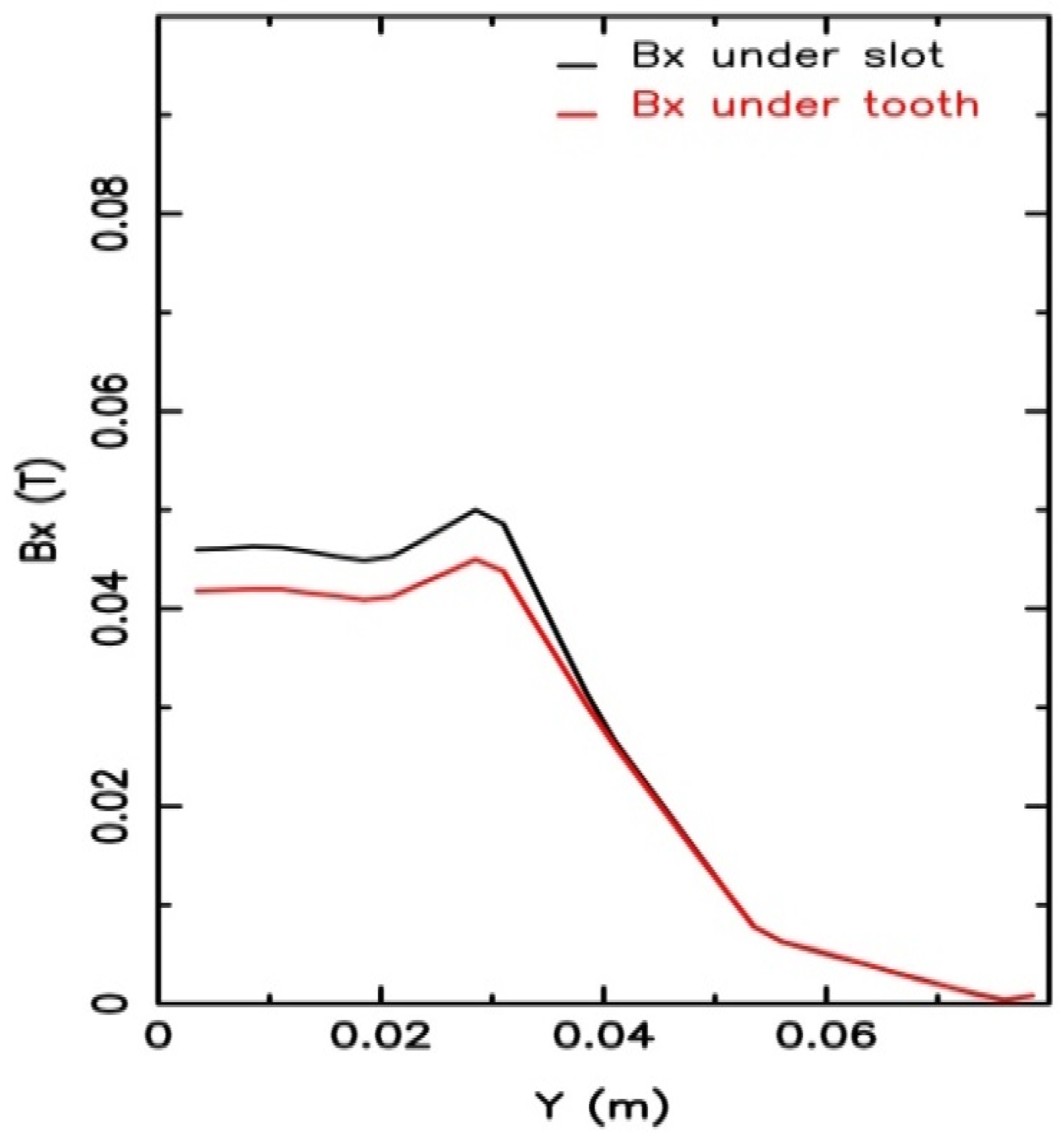
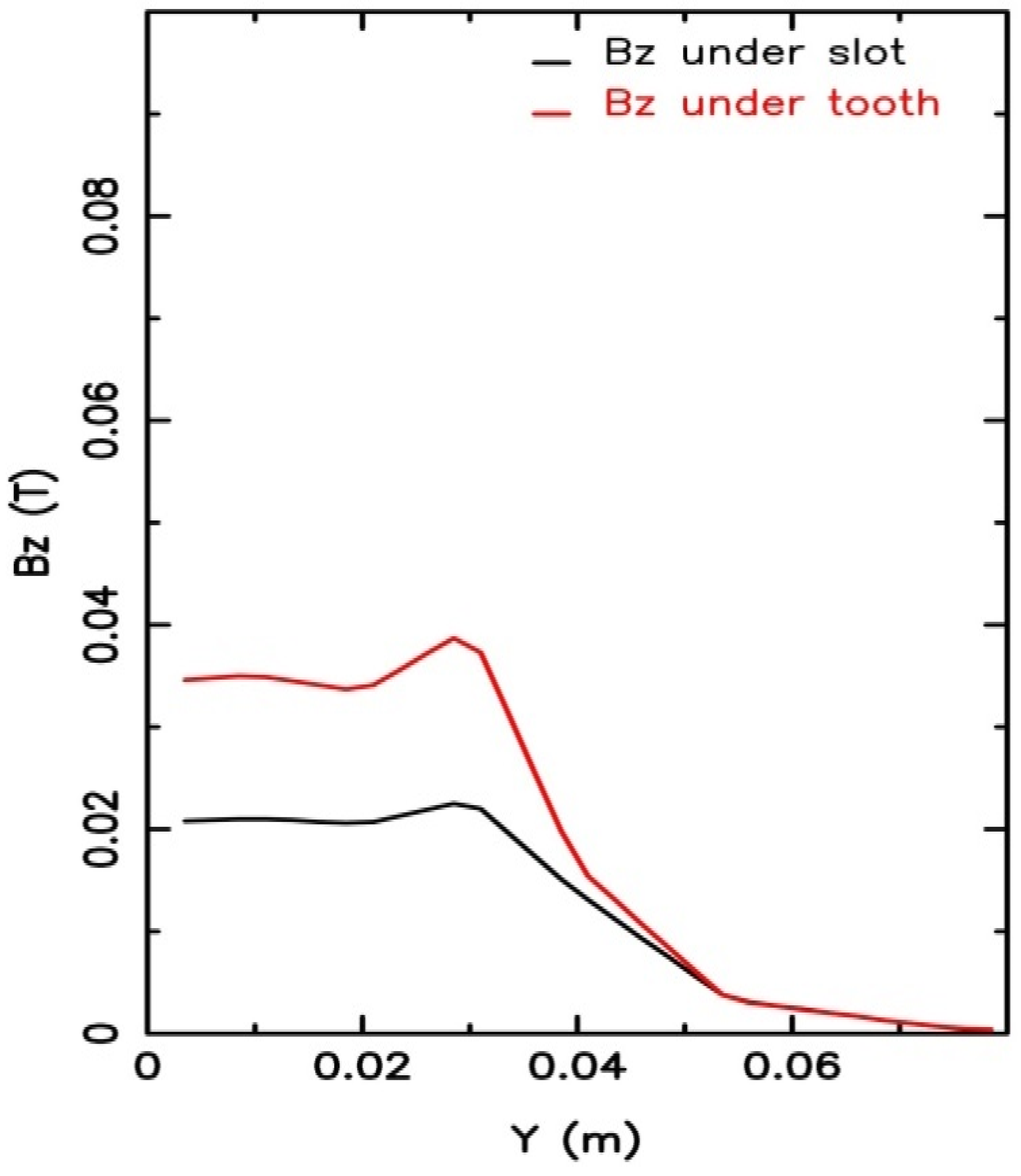
The vector potential at the sampling points of the BEM given in (19) can be written in matrix form as
{ A } C ( B ) = [ C ] { A } C ( F )
where [C] is a square matrix whose elements are either 0.25 or 0.
Taking into consideration that the normal unit vectors (n and n’) used in FEM and BEM are in opposite directions [20], then
A ( F ) n = A ( B ) n .
In matrix form, it is written as
{ q } C ( F ) = { q } C ( B )
Equation (24) can be rewritten as
{ q } C ( B ) = [ F ] 1 [ H ] { A } C ( B )
Substituting (28) into (30) results in
{ q } C ( B ) = [ F ] 1 [ H ] [ C ] { A } C ( F )
The problem nodes are numbered such that the boundary nodes come at the end, so that (8)–(10) can be written in matrix form as
S I I S I C S C I S C C { A I ( F ) } { A C ( F ) } = [ T ] [ D ] [ F ] 1 [ H ] [ C ] { A } C ( F )
where subscript I refers to the internal nodes and C refers to the boundary nodes.
The volume integrals involved in the system of linear equations in (32) are obtained numerically using the three-point Gaussian integration method [21].
Transferring the terms containing { A } C ( F ) from right to left and summing with the corresponding terms yields
S I I S I C S C I S C C + [ D ] [ F ] 1 [ H ] [ C ] { A I ( F ) } { A C ( F ) } = [ T ] 0
The set of equations in (33) are solved by the Gaussian elimination method. It was found [18] that iterative methods are not suitable for solving combined FEM-BEM matrices because the matrix is asymmetric.

6. Results

To verify the accuracy of the developed technique, two types of LIMs that have been published in the literature with measured values are adopted. Model-A [22] is a single sided LIM with an aluminum sheet rotor unbacked by iron, and in Model-B [6], the rotor conductor is backed by iron. The data for the two models are given in Table 1.

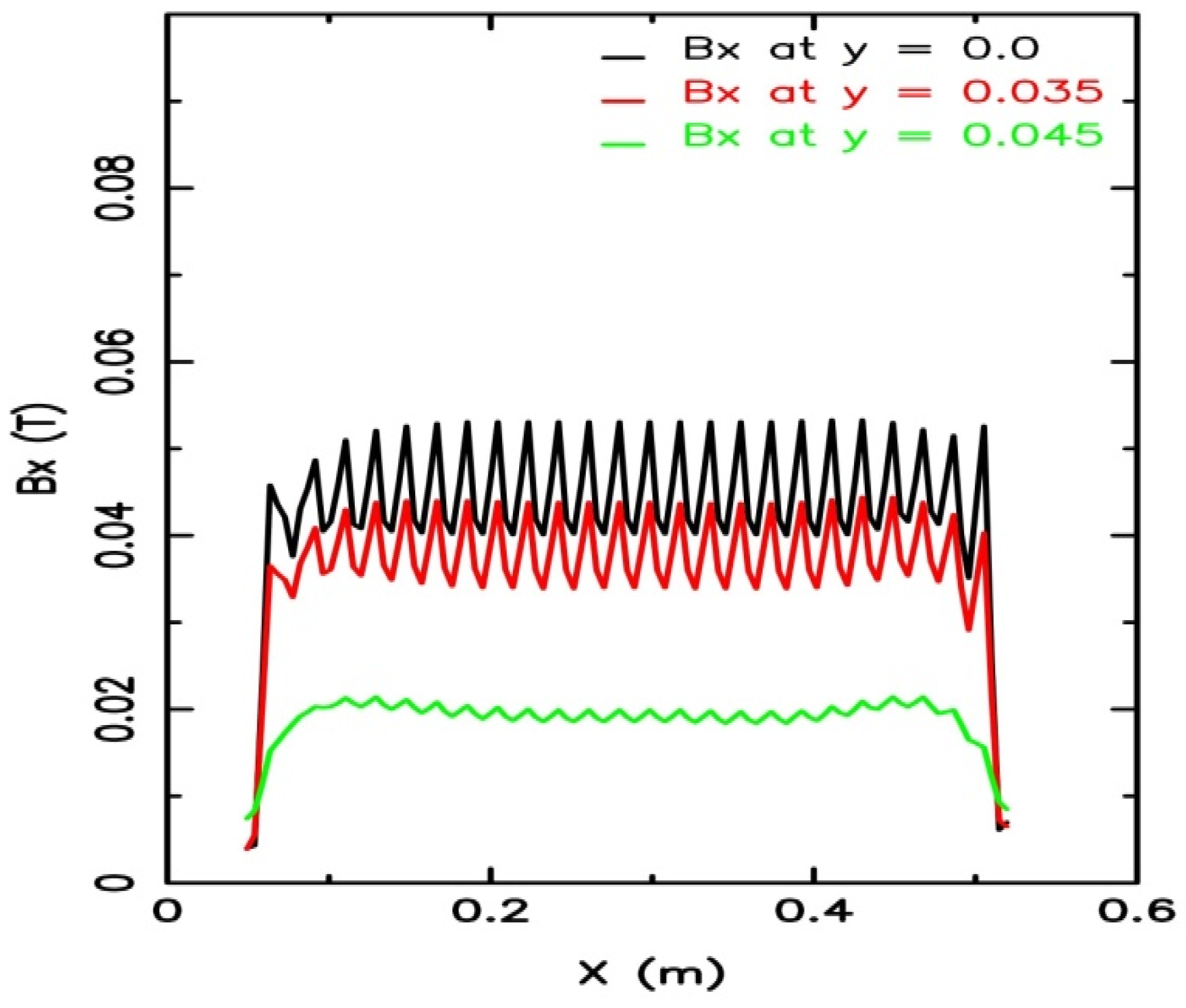
6.1. Model-A Results

The stator slots which contain the three-phase coils are represented as individual regions. The current in each slot is given as a complex value varying along the stator to produce the travelling current wave, as shown in Figure 3.
The value of the phase current in the i-th slot with peak amplitude I0 is given by
I = I 0 ( cos θ i j sin θ i )
where θi is the slot angle [23], given by
θ i = 2 π p s ( i 1 )
where p is the number of pole pairs and s is the total number of slots.
Making use of symmetry, and to minimize the computation time and storage memory requirements, one half of the model in the y direction is considered.
Computations were evaluated at different values of the outer boundary location (xo) starting from one half of a pole pitch (xo = xi), which was taken as the reference location, up to three pole pitches (xo = 6xi) from the machine ends.
Figure 4 shows the number of nodes used in the FEM model (in terms of the number of nodes used in the hybrid method model for xo = xi, where the number of nodes increases in polynomial form, which reflects the amount of computation time saved through the use of the hybrid method.
The magnetic flux density components computed in the air gap are given in Figure 5 and Figure 6, which show the variation in Bx and Bz components, respectively, along the x direction at mid-plane symmetry (where y = 0), with 5 mm from the edge (y = 35 mm, inside the stator) and 5 mm from the edge (y = 45 mm, outside the stator). Figure 7 and Figure 8 show the flux density components computed along the y direction under slot and under tooth. These figures illustrate the effect of slots and teeth on the flux density profile, showing noticeable edge effects in the transverse (y) direction.
The propulsion force Fx and the levitation force Fz are computed either in the air gap or in the rotor conductor elements. The hybrid FEM-BEM and FEM are applied, with both methods using the same outer boundary distance from the model edges, approximately half of the pole pitch. The results are validated against measurements from [22], as illustrated in Figure 9 and Figure 10. The hybrid FEM-BEM results exhibit a standard deviation of 4–5% compared to the measurements, while the FEM results show a standard deviation of approximately 30%. These findings demonstrate the higher accuracy of the hybrid FEM-BEM method. Furthermore, the results indicate that the hybrid FEM-BEM is independent of the outer boundary location, whereas FEM requires a sufficiently far boundary to achieve comparable accuracy.
Figure 11 and Figure 12 show the field contours at the transverse edge of the model. These contours represent magnetic flux lines, connecting points that have the same magnetic vector potential magnitude. The role of the hybrid method is clear, where contours intersect the outer boundary and the boundary vector potential values are obtained as part of the solution, whereas the FEM, which applies Dirichlet boundary conditions, results in tangential contours at which the magnetic vector potential is zero.

6.2. Model-B Results

Model-B is a single-sided LIM with back iron. Computations of the propulsion forces are performed using an exciting current of 11 A at a frequency of 30–50 Hz as given in [6]. Figure 13 shows the computed values of the forces versus velocity at different frequencies. The standard deviation between the computed values and the cited reference measurements is about 9–14%, which is considered reasonable.
The field contours at the transverse edge of the model (Figure 14) show the impact of the boundary element method in computing the boundary field values rather than assigning zero values.

7. Conclusions

The three-dimensional hybrid FEM-BEM method was adopted for the performance analysis of different models of LIMs at different frequencies. For an outer boundary location of about one half the pole pitch from the machine physical boundaries, it was found that FEM-BEM gives better results in comparison with the FEM with less computer storage. The achieved accuracy of the FEM-BEM in comparison with the cited reference measurements was within 4–5% for model-A and within 9–14% for model-B. In the FEM, a comparable accuracy was obtained when the outer boundary was located at about three pole pitches from the physical machine boundaries. We hoped that our analysis will prompt FEM commercial code designers to adopt this method. The proposed technique offers a reliable tool to help designers select suitable parameters for different design criteria.

Author Contributions

Methodology, L.Q.; Software, R.M.; Formal analysis, R.M.; Writing—review & editing, L.Q.; Supervision, L.Q. All authors have read and agreed to the published version of the manuscript.

Funding

This research received no external funding.

Data Availability Statement

The data presented in this study are openly available in Research Gate (https://dx.doi.org/10.2139/ssrn.5091790).

Conflicts of Interest

The authors declare no conflict of interest.

Appendix A

Making use of the vector identity [24],
a × ( b × c ) = ( a . c ) b ( a . b ) c
therefore,
v × × A φ = ( v . A ) ( v . ) A φ
φ can be expressed in terms of the magnetic vector potential A as
φ = ( v . A )
hence,
v × × A φ = ( v . ) A
Substituting (3) into (1) and (2), assuming all parameters vary sinusoidally with time and adopting complex notation to replace the time derivative, results in
× ( 1 μ × A ) + σ [ j ω A + ( v . ) A ] = J 0

References

  1. Yamaguchi, T.; Kawase, Y.; Yoshida, M.; Saito, Y.; Ohdachi, Y. 3-D Finite element analysis of a linear induction motor. IEEE Trans. Magn. 2001, 37, 3668–3671. [Google Scholar] [CrossRef]
  2. Ravanji, M.; Gheidari, Z. Design optimization of a ladder secondary single-sided linear induction motor for improved performance. IEEE Trans. Energy Convers. 2015, 30, 1595–1603. [Google Scholar] [CrossRef]
  3. Qaseer, L.; Marzouk, R. Hybrid finite element-boundary element analysis of a single-sided sheet rotor linear induction motor. IEEE Trans. Energy Convers. 2014, 29, 188–195. [Google Scholar] [CrossRef]
  4. Di, J.; Fletcher, J.E.; Fan, Y.; Liu, Y.; Sun, Z. Design and performance investigation of the double-sided linear induction motor with a ladder slot secondary. IEEE Trans. Energy Convers. 2019, 34, 1603–1612. [Google Scholar] [CrossRef]
  5. Lv, G.; Zhou, T.; Zeng, D.; Liu, Z. Influence of secondary constructions on transverse forces of linear induction motors in curve rails for urban rail transit. IEEE Trans. Ind. Electron. 2019, 66, 4231–4239. [Google Scholar] [CrossRef]
  6. Xu, W.; Sun, G.; Wen, G.; Wu, Z.; Chu, P.K. Equivalent circuit derivation and performance analysis of a single sided linear induction motor based on the winding function theory. IEEE Trans. Veh. Tech. 2012, 61, 1515–1525. [Google Scholar] [CrossRef]
  7. Li, D.; Li, W.; Zhang, X.; Fang, J.; Qiu, H.; Shen, J.; Wang, L. A New approach to evaluate influence of transverse edge effect of a single-sided HTS linear induction motor used for linear metro. IEEE Trans. Magn. 2015, 51, 8200404. [Google Scholar]
  8. Zeng, D.; Lv, G.; Zhou, T. Equivalent circuits for single-sided linear induction motors with asymmetric cap secondary for linear transit. IEEE Trans. Energy Convers. 2018, 33, 1729–1738. [Google Scholar] [CrossRef]
  9. Lv, G.; Zeng, D.; Zhou, T.; Degano, M. A complete equivalent circuit for linear induction motors with laterally asymmetric secondary for urban railway transit. IEEE Trans. Energy Convers. 2020, 36, 1014–1022. [Google Scholar] [CrossRef]
  10. Zeng, D.; Lv, G.; Zhou, T. Analysis of secondary losses and efficiency in linear induction motors with composite secondary based on space harmonic method. IEEE Trans. Energy Convers. 2017, 32, 1583–1591. [Google Scholar]
  11. Lv, G.; Zeng, D.; Zhou, T. Influence of ladder-slit secondary on reducing the edge effect and transverse forces in the linear induction motor. IEEE Trans. Ind. Electron. 2018, 65, 7516–7525. [Google Scholar] [CrossRef]
  12. Xu, W.; Elmorshedy, M.F.; Liu, Y.; Islam, R.; Allam, S.M. Finite-set model predictive control based thrust maximization of linear induction motors used in linear metros. IEEE Trans. Veh. Tech. 2012, 68, 5443–5458. [Google Scholar] [CrossRef]
  13. Tiunov, V. Linear induction motors tractive force components analysis with regard to the motors’ electromagnetic no-symmetry. In Proceedings of the 2019 International Multi-Conference on Industrial Engineering and Modern Technologies, Vladivostok, Russia, 1–4 October 2019; p. 19229138. [Google Scholar]
  14. Lu, Q.; Li, L.; Zhan, J.; Huang, X.; Cai, J. Design optimization and performance investigation of novel linear induction motors with two kinds of secondaries. IEEE Trans. Ind. Appl. 2019, 55, 5830–5842. [Google Scholar] [CrossRef]
  15. Xu, W.; Xiao, X.; Du, G.; Hu, D.; Zou, J. Comprehensive efficiency optimization of linear induction motors for urban transit. IEEE Trans. Veh. Technol. 2020, 69, 131–139. [Google Scholar] [CrossRef]
  16. Williamson, S.; Chan, E. Three-dimensional finite-element for problems involving time-varying fields, relative motion, and magnetic saturation. Proc. IEE A 1993, 140, 121–130. [Google Scholar]
  17. Nath, S. Finite Element and Boundary Element Analysis of Electromagnetic NDE Phenomena. Ph.D. Thesis, Iowa State University, Ames, IA, USA, 1992. [Google Scholar]
  18. Becker, A.A. The Boundary Element Method in Engineering A Complete Course; Mc-Graw-Hill: New York, NY, USA, 1992; Section 3.1. [Google Scholar]
  19. Beer, G.; Smith, I.; Duenser, C. The Boundary Element Method with Programming for Engineers and Scientists; Springer: New York, NY, USA, 2008. [Google Scholar]
  20. Fetzer, J.; Kurz, S.; Lehner, G. The Coupling of boundary elements and finite elements for nondestructive testing applications. IEEE Trans. Magn. 1997, 33, 677–681. [Google Scholar] [CrossRef]
  21. Chandrupatla, T.; Chandrupatla, T.R.; Belegundu, A. Introduction to Finite Elements in Engineering, 3rd ed.; Prentice-Hall: Upper Saddle River, NJ, USA, 2002; Section 7.3. [Google Scholar]
  22. Al-Maayouf, M.A. A Study of a Linear Induction Motor Using Alternative Models. Ph.D. Dissertation, Department of Electrical Engineering, The City University, London, UK, 1981. [Google Scholar]
  23. Say, M.G. The Performance and Design of Alternating Current Machines, 3rd ed.; Isaac Pitman & Sons: London, UK, 1965; p. 201. [Google Scholar]
  24. Stratton, J.A. Electromagnetic Theory; McGraw-Hill Book Co.: New York, NY, USA,, 1941; Section 1.9. [Google Scholar]
Figure 1. The three-dimensional model for the LIM.
Electronics 14 01261 g001
Figure 2. Proposed treatment of boundary element singularity.
Electronics 14 01261 g002
Figure 3. Current wave along the stator for Model-A.
Electronics 14 01261 g003
Figure 4. Normalized number of nodes versus outer boundary location for Model-A.
Electronics 14 01261 g004
Figure 5. Air-gap flux density component Bx along the x direction.
Electronics 14 01261 g005
Figure 6. Air-gap flux density component Bz along the x direction.
Electronics 14 01261 g006
Figure 7. Air-gap flux density component Bx along the y direction.
Electronics 14 01261 g007
Figure 8. Air-gap flux density component Bz along the y direction.
Electronics 14 01261 g008
Figure 9. Propulsion force versus slip for Model-A.
Electronics 14 01261 g009
Figure 10. Levitation force versus slip for Model-A.
Electronics 14 01261 g010
Figure 11. Field contours at the transverse edge of Model-A using FEM-BEM.
Electronics 14 01261 g011
Figure 12. Field contours at the transverse edge of Model-A using FEM.
Electronics 14 01261 g012
Figure 13. Propulsion force versus velocity for Model-B at 30–50 Hz.
Electronics 14 01261 g013
Figure 14. Field contours at the transverse edge of Model-B using FEM-BEM.
Electronics 14 01261 g014
Table 1. Machine data.
QuantityModel AModel B
Number of poles46
Number of phases33
Frequency (Hz)5050
Stator length (mm)448798
Stator height (mm)7699
Stator width (mm)80100
Pole pitch (mm)112117
Slot pitch (mm)18.66719.5
Slot width (mm)1311.7
Slot depth (mm)3830
Air gap length (mm)9.510
Number of turns per slot10036
Slot per pole per phase22
Phase current r.m.s (A)511
Type of rotorAluminumAluminum
Thickness of rotor (mm)3.1755
Rotor width (mm)240160
Conductivity of rotor (S/m)3.54 × 1073.54 × 107
Back iron width (mm)---21
Disclaimer/Publisher’s Note: The statements, opinions and data contained in all publications are solely those of the individual author(s) and contributor(s) and not of MDPI and/or the editor(s). MDPI and/or the editor(s) disclaim responsibility for any injury to people or property resulting from any ideas, methods, instructions or products referred to in the content.

