1. Introduction
The exponential growth of geospatial data, particularly Point of Interest (POI) data, has created significant opportunities for advancing location-based services (LBS) [
1]. Applications such as intelligent transportation [
2], urban planning [
3], and business analytics [
4] rely heavily on an accurate and comprehensive understanding of POIs. A POI inherently encapsulates two fundamental types of information: intrinsic attributes such as geographic coordinates and categories and spatial context, which reflects the relationships among POIs within their environment [
5]. Robust information representations enable downstream models to better understand POI semantics, uncover spatial patterns, and generalize across diverse geospatial contexts. Effectively capturing and integrating these diverse sources of information into feature vectors is critical for downstream tasks such as classification [
6], prediction [
7], and recommendation [
8].
To address the need for effective POI representation, existing methods primarily focus on modeling intrinsic attributes and spatial contexts. For intrinsic attributes, coordinate encoders are used to process geographic features [
9], while text encoders capture semantic information from POI categories and descriptions [
10]. These encoded features are then fused to form unified representations [
5]. For spatial context, graph neural networks (GNNs) have become a dominant approach due to their ability to model relational dependencies among POIs [
11,
12,
13]. By aggregating information from neighboring POIs, GNNs enable the encoding of spatial structures and dependencies.
Despite their utility, POI datasets present unique challenges, the most notable being label sparsity, which significantly hampers the effectiveness of supervised learning approaches. In POI datasets, labels are typically limited to categorical information, which is often incorporated as part of the input features rather than being used as targets for learning tasks. This lack of diverse and task-specific labels restricts the range of meaningful supervised tasks that can be formulated, making it challenging for models to learn reliable representations. These limitations have driven increasing interest in self-supervised learning (SSL), a paradigm that derives meaningful representations through pretext tasks leveraging the inherent structure of the data [
14]. SSL has gained substantial traction in domains such as computer vision [
15,
16,
17,
18] and natural language processing [
19,
20,
21], where it has successfully mitigated the dependence on labeled data and unlocked novel opportunities for representation learning.
Self-supervised learning (SSL) methods for POI representation can be broadly categorized into skip-gram-based methods and GNN-based methods, each with distinct strengths and limitations. Skip-gram-based methods draw inspiration from Word2Vec [
22], treating the spatial neighborhood of a POI as its context and minimizing errors in predicting this context using POI embeddings [
23,
24]. These methods excel at capturing localized spatial relationships and category-level similarities. GNN-based methods construct graphs based on spatial proximity and leverage graph neural networks to encode local structures into latent representations [
25,
26]. These approaches offer greater flexibility, allowing for predictive tasks such as reconstructing node attributes or inferring relationships. While both approaches offer valuable insights, they face notable limitations. Skip-gram methods are constrained by their reliance on local pairwise relationships, which restrict their ability to capture more complex spatial structures. GNN-based contrastive learning relies heavily on the quality of graph construction, which determines how well spatial relationships are represented, and the design of pretext tasks, which guide the learning process.
Recently, masked modeling, a powerful SSL paradigm, has emerged as a promising direction for representation learning. By masking and reconstructing parts of the data, this approach enables models to capture contextual dependencies and semantic features effectively. Notable examples include masked language modeling [
27,
28] and masked image modeling [
29,
30], which have demonstrated significant success in natural language processing and computer vision by designing tasks that exploit the inherent structure of textual and visual data. Inspired by these advancements, researchers have begun to explore the potential of masked modeling for POI representation learning.
For POI data, masked modeling has primarily been implemented through sequence-based approaches, such as GeoBERT [
31] and SpaBERT [
32]. These methods transform POI attributes into textual sequences and apply masked language modeling to predict missing components. While effective in some scenarios, these approaches often neglect or oversimplify the spatial relationships among POIs during the transformation process, leading to a partial loss of critical spatial context. This limitation highlights the need for innovative methods that can simultaneously preserve and leverage the structural integrity of POI data for more comprehensive representation learning.
To address these limitations, this paper introduces MaskPOI, a novel self-supervised learning framework that combines the strengths of graph neural networks (GNNs) and masked modeling. MaskPOI is designed to jointly capture both the spatial context and intrinsic attributes of POIs. By leveraging GNNs to model spatial relationships and implementing a graph-specific masking strategy, MaskPOI ensures the preservation of structural and spatial integrity while enabling robust and generalizable representation learning.
The proposed framework consists of two main components: An edge mask-based graph autoencoder, which predicts the existence of edges in the graph. This module focuses on modeling the spatial topology of POIs and uncovering hidden spatial relationships that may not be explicitly annotated in the data. A feature mask-based graph autoencoder, which masks and reconstructs node features. This module allows the model to deeply explore attribute characteristics, leading to richer and more distinguishable representations. Both components are integrated into a GNN encoder–decoder architecture, where the GNN encoder extracts graph-level representations and the edge and feature decoders reconstruct spatial and attribute relationships, respectively. These self-supervised tasks enable the model to learn high-quality POI representations without requiring explicit supervision, capturing the complex interplay between spatial and intrinsic attribute information.
The primary contributions of this paper are summarized as follows:
We propose a self-supervised learning framework based on graph neural networks, which jointly learns the node and edge features in the graph to capture both spatial and attribute information between POIs. This approach generates high-quality POI representations by effectively utilizing the structural characteristics of POI data, thereby improving the accuracy and generalization ability of representation learning.
We design an edge mask-based graph modeling task that enhances the modeling of spatial relationships between POIs by predicting the existence of edges. This approach captures the spatial topology of POIs and uncovers potential spatial relationships that may not be explicitly labeled, thereby improving the model’s ability to characterize spatial interactions.
We propose a feature mask-based graph modeling task, which focuses on learning by masking and reconstructing POI node features. This method enables the deep exploration of POI attribute features, resulting in richer and more distinguishable representations that significantly improve performance on downstream tasks.
We conduct extensive experiments in Beijing and Xiamen, evaluating the proposed framework on two downstream tasks: functional zone classification and population density prediction. The results demonstrate the superiority of MaskPOI in practical applications. Additionally, through ablation experiments, we provide an in-depth analysis of each module’s effectiveness, further validating the innovation and practicality of our approach.
3. Problem Formulation
Let represent a collection of t POIs. Each POI (e.g., a public park or a shopping mall) is characterized by its two-dimensional geographic coordinates and a categorical set . The set is expressed as , where specifies the category of at the j-th hierarchical level, and denotes the depth of the hierarchy (commonly for standard POI datasets). For instance, a POI’s categories might include , illustrating the hierarchical structure where broader first-level categories encompass multiple specific second-level categories.
POI representation learning aims to map each into a low-dimensional vector space such that the vector effectively captures the spatial, categorical, and potentially other contextual attributes of the POI. The goal of representation learning is to ensure that the learned embeddings can be utilized in downstream tasks, such as POI recommendation, clustering, or spatial analysis, while preserving meaningful relationships between POIs, including geographic proximity, categorical similarity, and other latent connections.
4. Methodology
4.1. Overview of MaskPOI
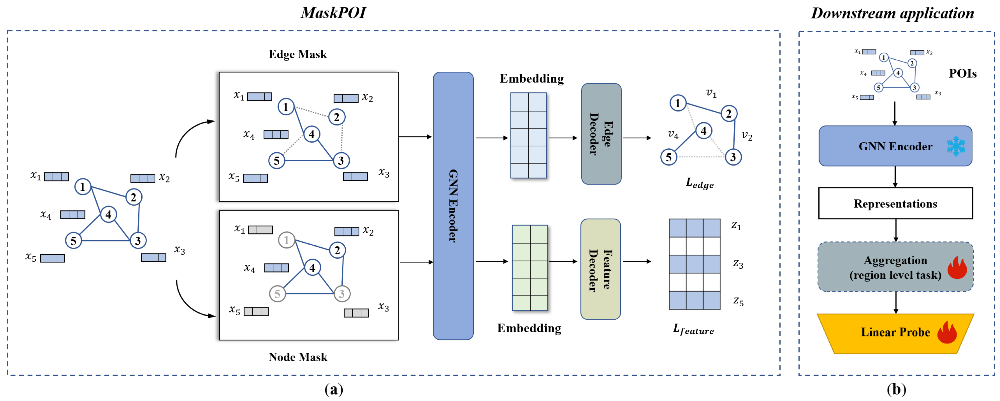
MaskPOI is a self-supervised graph neural network framework designed for POI representation learning. It adopts a dual-branch architecture to simultaneously leverage spatial relationships and feature dependencies within the constructed POI graph structure. The overall architecture of MaskPOI is depicted in
Figure 1a. The core idea of MaskPOI is to randomly mask edges or node features in the graph, process the graph through the GNN encoder, and then predict the masked components using separate decoders.
Firstly, a graph is constructed where the nodes represent POIs and the edges capture the spatial relationships between them. Each POI node is initialized with a feature vector that encodes its attributes, including the location and category.
The core of MaskPOI is the GNN encoder, which aggregates information from neighboring nodes to produce contextualized node embeddings. To enhance the robustness of the learned embeddings, MaskPOI introduces two key self-supervised learning mechanisms as follows: Edge Masking: A subset of edges is randomly masked, and the model learns to reconstruct these masked connections using the encoded node embeddings. This mechanism encourages the model to infer missing relationships based on the structural information in the graph. Feature Masking: A subset of features is randomly masked, and the model is trained to reconstruct these masked features. This task forces the model to understand and predict the underlying characteristics of POIs based on their graph context.
Finally, the outputs from the GNN encoder are fed into two separate decoders: the edge decoder, which predicts the presence of masked edges, and the feature decoder, which reconstructs the masked feature values. The combination of these two reconstruction tasks forms the self-supervised training objective, ensuring the learned embeddings capture both structural- and feature-level dependencies.
MaskPOI’s architecture is designed to generalize across various downstream tasks, as shown in
Figure 1b.The GNN encoder produces task-agnostic representations for individual POIs, which can be directly utilized for node-level tasks such as POI classification or clustering. For region-level tasks, such as urban functional zone classification or population density prediction, an additional aggregation step combines embeddings of POIs within the same region to capture macro-scale patterns. The resulting representations, whether node level or region level, are passed to a simple linear probe for efficient task-specific predictions, showcasing the versatility of MaskPOI across various application scenarios.
4.2. Graph Construction and POI Feature Generation
To accurately represent the Points of Interest (POIs) and their spatial interconnections, we constructed a topological graph grounded in the road network. This design captures both the functional diversity of POIs and their real-world spatial relationships.
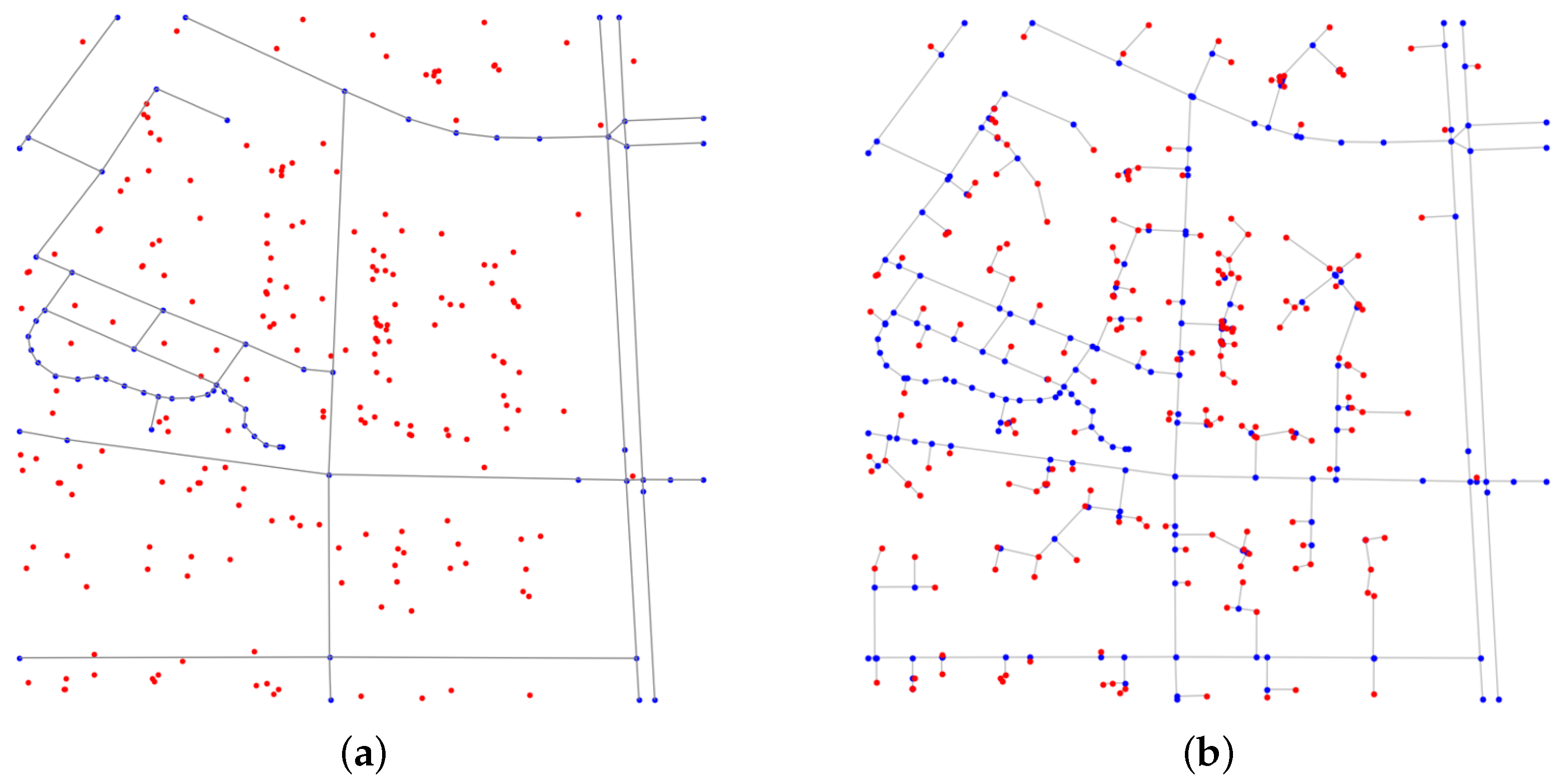
The graph construction process begins by dividing the study area into spatial grids. In each grid, roads and their vertices are added as edges and nodes to form the initial structural framework, as shown in
Figure 2a. These nodes do not carry any attribute information. POIs, which are not located directly on roads, are connected to the road network based on the shortest distance to road segments. If the nearest point on a road segment does not coincide with an existing road vertex, a new intersection node is added at this location. The POI is then connected to this newly created node, ensuring an accurate representation of spatial relationships, as shown in
Figure 2b.
After constructing the topological graph, we need to generate the initial features for the nodes based on the POI attributes. The initial features for POIs combine semantic and spatial information to enable robust representation learning. Semantic attributes, including a three-level categorical hierarchy (e.g., food service, fast food restaurant, McDonald’s), are encoded using a pre-trained Bidirectional Encoder Representation from Transformers (BERT) model [
28]. BERT is pre-trained on a large corpus using Masked Language Modeling (MLM) and Next Sentence Prediction (NSP) tasks, enabling it to learn deep contextual representations. The model processes input text by tokenizing it using word encoding, adding special tokens ([CLS]), and passing the sequence through multiple Transformer layers. The [CLS] token’s output is commonly used as a global sentence representation, while other tokens capture token-level semantics. By extracting 768-dimensional embeddings from the [CLS] token of each category description, BERT effectively captures semantic relationships between different POI categories.
To incorporate spatial information, the geographic coordinates of POIs are normalized within the bounding box of the grid. These normalized coordinates, consisting of two values (latitude and longitude), are concatenated with the BERT-based semantic embeddings. As a result, the final feature vector for each POI node has a total of
dimensions, effectively capturing both spatial and semantic characteristics. The process can be expressed by the following formula:
where
represent the three-level categorical attributes of the POI;
denotes the embedding generated by the BERT model for the category
C;
are the geographic coordinates of the POI; and
are the minimum and maximum values of the grid.
Road intersection nodes, which lack semantic attributes, are assigned feature vectors consisting of normalized coordinates concatenated with zero vectors matching the dimensionality of the BERT embeddings. This uniform feature dimensionality across all nodes ensures consistency and facilitates the learning process.
By integrating POIs into road networks and leveraging semantic embeddings from BERT, the constructed graph effectively combines spatial and attribute information. This design not only reflects real-world spatial interactions but also enhances the interpretability and utility of the learned POI representations. The impact of different graph construction methods and feature encoding strategies is discussed in
Section 7.1 and
Section 7.2. We compared alternative graph construction techniques, such as Delaunay triangulation, with the proposed road-based method. Additionally, the effectiveness of the BERT-based embeddings was evaluated in comparison to simpler encoding approaches, such as one-hot encoding.
4.3. Edge Mask Modeling
We adopted an edge-wise random masking strategy to facilitate the edge prediction task in MaskPOI. Given a graph , we randomly sampled a subset of edges as the masked edges and retained the remaining edges to construct the visible graph . The relationship between these components satisfies , ensuring that the masked and visible graphs together represent the original graph structure.
The masked edges
are sampled based on a Bernoulli distribution, where each edge in
E is independently selected for masking with a probability
p. Formally, the sampling process can be expressed as:
where
defines the edge masking ratio. This ratio determines the proportion of edges that are removed and thus controls the difficulty of the edge reconstruction task. A higher
p introduces more masked edges, forcing the model to rely more heavily on the remaining graph context for prediction.
The GNN encoder in the proposed MaskPOI framework is implemented using a multi-layer Graph Convolutional Network (GCN), which is designed to capture both local and global node features within the graph. The encoder takes the graph structure (edge index) and node features as inputs and processes them through multiple GCN layers. Each layer propagates and aggregates neighborhood information to produce richer node embeddings. The shared GNN encoder is responsible for producing node embeddings for both the edge-masking and feature-masking tasks. For each task, the input graph is processed by the encoder, and the resulting node embeddings are passed to the respective decoders.
The edge decoder in MaskPOI reconstructs the masked edges by predicting their existence based on the node embeddings generated by the GNN encoder. For a given masked edge
, where
, the decoder first combines the node embeddings
and
through an elementwise product:
where
are the
d-dimensional embeddings of nodes
u and
v, and ⊙ represents the elementwise product. This operation captures the pairwise interaction between the nodes.
The combined representation
is passed through a multi-layer perceptron (MLP) to model non-linear relationships, and a sigmoid activation function is applied to compute the probability of the edge’s existence.
where
is the sigmoid function, and
represents the predicted likelihood of the edge
existing in the graph.
4.4. Feature Mask Modeling
To facilitate the self-supervised learning task of feature reconstruction, MaskPOI employs a feature masking strategy combined with a dedicated decoder for reconstructing node attributes. Given the input node feature matrix X, the masking process selects a portion of the nodes to mask based on a predefined masking ratio p. For each selected node, its features are replaced with a learnable masking token.
The masked node features and the graph structure are input into the shared GNN encoder mentioned above. The shared encoder ensures that the learned embeddings capture both structural- and feature-level dependencies. The output embeddings Z from the encoder serves as the input for the feature decoder, enabling the reconstruction of the original node features. The feature decoder in MaskPOI is implemented using GCN instead of a standard MLP. By leveraging the GCN layers, the decoder incorporates structural relationships from the graph, effectively utilizing neighborhood information to reconstruct features.
4.5. Training Objective
The training objective of MaskPOI aims to learn robust POI representations through self-supervised learning by optimizing two primary reconstruction tasks: edge reconstruction and feature reconstruction. By addressing these tasks simultaneously, the model effectively captures both the structural relationships and the feature-level dependencies among POIs.
Edge Reconstruction Task: The edge reconstruction task aims to predict the existence of masked edges using the latent node representations. The edge decoder is tasked with predicting whether the masked edges (positive samples) exist, as well as predicting a set of randomly sampled non-existent edges (negative samples). The edge reconstruction loss is computed by comparing the predicted probabilities of the edges’ existence with the actual labels, as follows:
where
and
represent the decoder’s predicted scores for the masked edges and the randomly sampled non-existent edges, respectively, and
denotes the sigmoid activation function. The first term penalizes the incorrect predictions of the masked edges (positive samples), while the second term penalizes the incorrect predictions of the negative edges (non-existent samples), encouraging the model to learn to distinguish between actual edges and random samples.
Feature Reconstruction Task: The feature reconstruction task aims to reconstruct the masked node features using the graph structure and the remaining visible node features. The feature decoder predicts the original feature values for the masked nodes. The reconstruction loss is computed based on the cosine similarity between the reconstructed feature vector and the original feature vector for each masked node:
where
is the reconstructed feature vector for node
i, and
is the ground truth feature vector for node
i. The cosine similarity loss measures how similar the reconstructed and original feature vectors are, encouraging the model to preserve important feature-level information while learning the dependencies among POIs.
Total Training Loss: The total training objective combines both the edge reconstruction loss and the feature reconstruction loss as follows:
This multi-task learning objective allows the MaskPOI model to learn both structural and feature dependencies in the graph, resulting in robust and generalizable POI embeddings.
5. Experiment Settings
5.1. Study Areas and Data
This research selects Beijing and Xiamen as representative cities of northern and southern China, respectively. The study area in Beijing focuses on the central urban area, approximately within a 9 km square around Tiananmen Square, effectively covering the city’s core, as illustrated in
Figure 3a. This region represents the economic and administrative center of Beijing, characterized by a high degree of urbanization and a dense concentration of POIs, including commercial, residential, cultural, and governmental facilities. The study area in Xiamen is confined to Xiamen Island, as illustrated in
Figure 3b. Xiamen Island serves as the political, economic, and cultural hub of Xiamen, exhibiting a compact urban structure. The island’s unique geographic setting and its role as a major port city contribute to its distinct urban dynamics compared to Beijing.
The POIs used in this study were collected from Amap
https://lbs.amap.com/ (accessed on 20 February 2025) and represent a wide range of urban facilities and services. A total of 206,331 POIs were included in the dataset for Beijing, categorized into a hierarchical structure with three levels as follows: 23 first-level categories (e.g., food services, retail, public services), 193 second-level categories (e.g., fast food restaurants, shopping malls, government agencies), and 587 third-level categories (e.g., McDonald’s, Starbucks, local grocery stores). A total of 48,282 POIs were included in the dataset for Xiamen, categorized into 14 first-level categories, 93 second-level categories, and 437 third-level categories. Each POI is associated with its geographic coordinates and three category labels from the hierarchical structure, providing both spatial and functional context for analysis. In addition, the latest OpenStreetMap (OSM) road vector data for Beijing was used in this study
https://www.openstreetmap.org/ (accessed on 20 February 2025).
To construct the topological network, both POIs and roads were divided into grids with a cell size of 500 m. This grid-based approach allows for efficient spatial analysis by associating POIs and roads with specific grid cells, facilitating the creation of a topological network that captures the relationships between geographic features within the study area.
Similar to the approach in study [
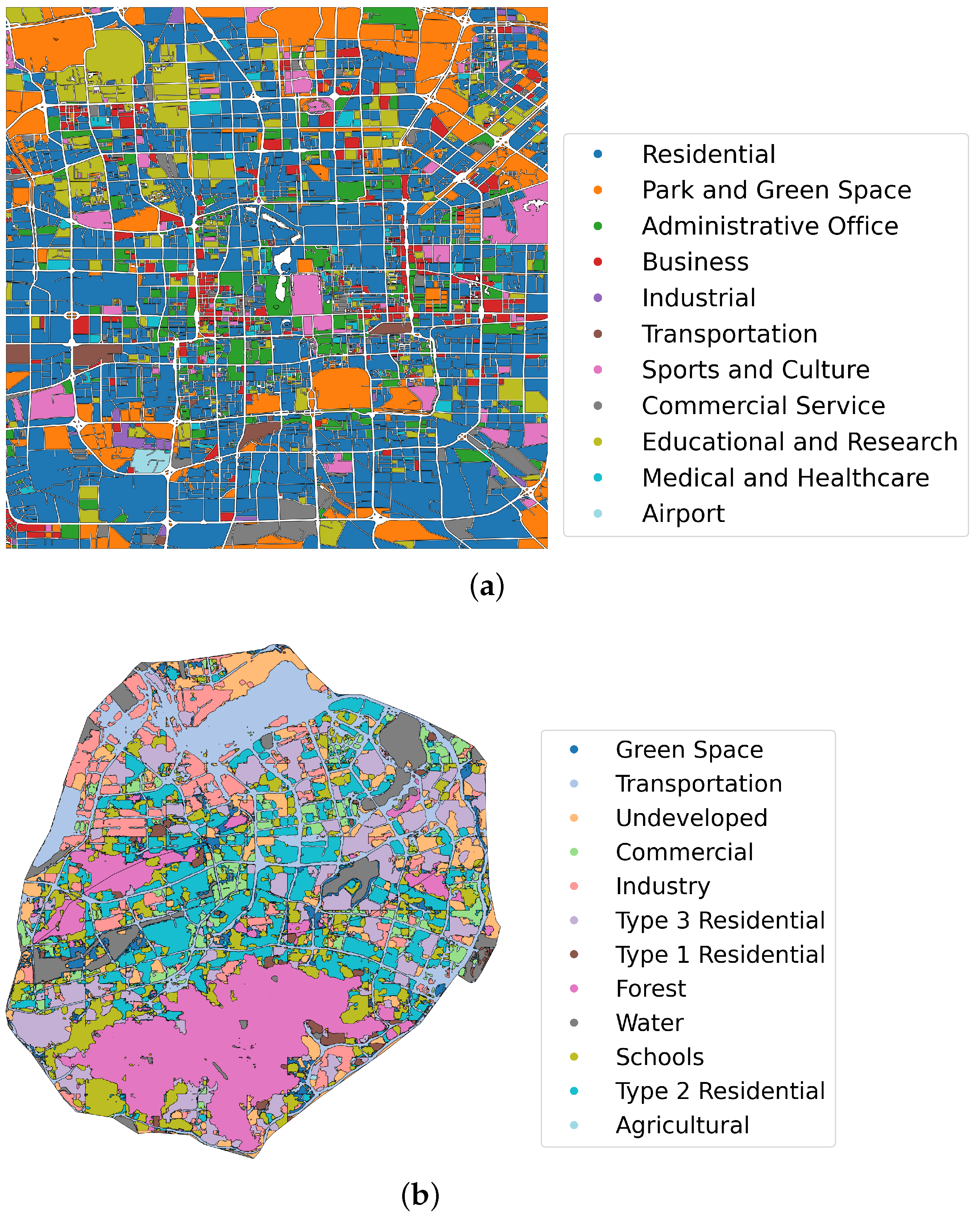
50], we validated the learned POI representations on two downstream tasks: urban functional zone classification and population density prediction. The ground truth data of urban functional zone classification are shown in
Figure 3. The urban functions of Beijing are sourced from EULUC-China
https://data-starcloud.pcl.ac.cn/resource/7 (accessed on 20 February 2025) [
51]. EULUC-China is a comprehensive land use dataset for China, developed through the integration of remote sensing imagery and GIS, providing detailed information on land use types across the country. It includes 12 categories, including transportation, road, sports, and cultural, park and green space, medical and healthcare, commercial service, business, residential, industrial, educational and research, airport, administrative office. The urban functions of Xiamen are derived from the Urbanscape Essential Dataset of Peking University
http://geoscape.pku.edu.cn/en.html (accessed on 20 February 2025), which offers comprehensive spatial data on 12 urban functions across the study areas. These include forest, water, undeveloped land, transportation, green space, industrial areas, educational and governmental facilities, commercial zones, residential (type 1, 2, 3), and agricultural land. The dataset was compiled using a combination of remote sensing data, POI information, and human-driven corrections and adjustments. Each grid in the study area is assigned a 12-dimensional vector, representing the proportion of urban function in each of these categories. This vector is computed by overlaying the spatial grid with the urban function dataset, ensuring that each grid captures the relative distribution of these functional zones.
The population density data is sourced from WorldPop. We utilized the most recent dataset, representing the spatial distribution of China’s population in 2020 with a resolution of 100 m
https://hub.worldpop.org/geodata/summary?id=49730 (accessed on 20 February 2025). By overlaying this dataset with the spatial grid, we calculated the population density for each grid cell, expressed as the number of people per 100 square meters.
5.2. Implementation Details of MaskPOI
The implementation of MaskPOI involved the systematic tuning of hyperparameters and the selection of model components to optimize performance. For edge masking, a range of mask rates between 0.1 and 1.0 was explored, with a rate of 0.3 selected as optimal. Similarly, the feature masking rates were tuned between 0.1 and 0.9, leading to a chosen rate of 0.6. The dimensionality of node representations was adjusted between 32 and 256, with the best performance observed at a dimension of 128. Both the GNN encoder and the feature decoder were implemented as single-layer Graph Convolutional Networks (GCNs). The analysis of these parameters can be found in
Section 6.2.
The training process employed a learning rate of with a cosine annealing scheduler, a weight decay of , and a batch size of . The model was trained for 100 epochs on an NVIDIA A800 GPU with 80 GB of memory, enabling the efficient handling of large-scale graph data. For the experiments conducted on the Beijing dataset, the model used approximately 76,524 MB of GPU memory, with a training time of around 10 min. For the Xiamen dataset, the model consumed 16,278 MB of GPU memory, and the training time was approximately 3 min.
For the downstream experiments, we used Set2Set [
24,
52,
53] to obtain the region representations. We randomly selected 80% of the data for training, 10% for validation, and 10% for testing. Each experiment was run 5 times with random initialization. The mean and standard deviation are reported.
5.3. Compare Methods
To evaluate the effectiveness of our proposed approach, we compared it with several state-of-the-art methods for POI representation learning and graph self-supervised learning. These methods include the following:
Semantic Embedding [
24]: A method that utilizes textual or categorical attributes of POIs to learn representations, focusing on semantic similarity between POIs.
DeepWalk [
54]: A classic graph-based representation learning algorithm that performs random walks on graphs to generate node embeddings. It is effective for learning structural information and is commonly used in spatial and networked data analyses.
Node2Vec [
55]: An extension of DeepWalk that introduces a biased random walk strategy to capture both local and global graph structures, enabling the embedding to encode more diverse contextual information.
DGI (Deep Graph Infomax) [
39]: A graph self-supervised learning method that maximizes mutual information between local node embeddings and the global graph representation. This approach has proven effective in unsupervised learning on graph data.
GAE (Graph Autoencoder) [
46]: A graph neural network-based autoencoder model that learns low-dimensional representations by reconstructing the graph structure. It is commonly used for unsupervised node and graph representation learning.
GraphMAE (Graph Masked Autoencoder) [
49]: A self-supervised graph learning model that uses masked graph modeling to learn robust embeddings by reconstructing missing node or edge features.
MaskGAE (Masked Graph Autoencoder [
56]: An advanced variant of graph autoencoder that integrates masking mechanisms during encoding to enhance the model’s ability to generalize and capture latent patterns in graph data.
UniMP (Unified Message Passing Model) [
57]: A model that unifies feature and label propagation within a Graph Transformer and uses a masked label prediction strategy. It adopts the vanilla multi-head attention of the Transformer in graph learning, taking the node features and label embeddings as input for information propagation between nodes.
GCA (Graph Contrastive Learning with Adaptive Augmentation) [
58]: A novel unsupervised graph representation learning method that generates two graph views via adaptive augmentation at the topology and node-attribute levels and uses a contrastive loss to train the model and outperforms state-of-the-art methods in node classification tasks.
5.4. Evaluation Metrics
For the evaluation of the proposed methods, we adopted different metrics tailored to the tasks. To measure the similarity between vectors in the urban functional composition classification task, we employed the following metrics, ↓ indicates that smaller values are better, while ↑ indicates that larger values are better.
L1 Distance (L1)↓: The L1 distance between the estimated functional composition vector
and the ground truth vector
for region
i is defined as:
Kullback–Leibler Divergence (KL)↓: The KL divergence measures the difference between the estimated functional composition
and the ground truth
:
Cosine Similarity (Cosine)↑: The cosine similarity between the estimated functional composition
and the ground truth
is computed as:
where
is the estimated proportion of the function type
that region
i bears, and
is the corresponding ground truth proportion; satisfy
and
.
For the regression task of predicting the population density, we used the following metrics:
Root Mean Square Error (RMSE)↓: The RMSE evaluates the standard deviation of the prediction errors between the estimated population density
and the ground truth
for all regions, defined as:
Mean Absolute Error (MAE)↓: The MAE computes the average magnitude of errors between the estimated population density
and the ground truth
, defined as:
Coefficient of Determination (
)↑: The
metric assesses the proportion of variance in the ground truth population density
that is predictable from the estimated population density
, defined as:
where
is the estimated population density for region
i,
is the corresponding ground truth,
is the mean of the ground truth population density, and
N is the total number of regions.
These metrics comprehensively evaluate the effectiveness of the proposed methods across both classification and regression tasks, providing robust and interpretable performance measures.
6. Results
6.1. Performance
We evaluated the performance of MaskPOI on two downstream tasks: the urban functional zone classification and population density prediction in Beijing and Xiamen, respectively.
The result of Beijing is shown in
Table 1. MaskPOI outperforms all other models across most metrics on both tasks. In urban functional zone classification, MaskPOI achieves the best results in KL divergence (0.834 ± 0.013) and cosine similarity (0.761 ± 0.003). It also performs exceptionally well in population density prediction, achieving the lowest RMSE (0.133 ± 0.003) and MAE (0.1 ± 0.002), along with the highest
value (0.436 ± 0.005). These results demonstrate the superior ability of MaskPOI to capture complex spatial and functional relationships in the data, highlighting its effectiveness in both tasks.
In contrast, models such as DeepWalk and Node2Vec show relatively lower performance across all metrics, particularly in the urban functional zone classification task. While Semantic exhibits promising results in L1, MaskPOI consistently shows superior performance, making it the most effective model for these types of POI-based tasks.
The result of Xiamen is shown in
Table 2. MaskPOI demonstrates superior performance across both urban function classification and population prediction tasks. It achieves the lowest KL divergence (0.791) for urban function classification, along with the highest cosine similarity (0.703), indicating its ability to effectively capture urban function patterns. For population prediction, MaskPOI also excels, attaining the lowest RMSE (0.173) and MAE (0.138), and the highest
(0.639), showing its robustness in accurately predicting population densities. These results highlight the effectiveness of incorporating POI data and advanced masking techniques in enhancing both classification and regression tasks.
In comparison, other methods such as Semantic, GCA, and GAE fall short of MaskPOI in terms of overall accuracy and error reduction. DGI shows competitive results, while others like DeepWalk and Node2Vec lag behind in both tasks, demonstrating lower cosine similarity and higher prediction errors. Overall, MaskPOI stands out as the most effective approach, consistently delivering the best results across most evaluation metrics.
6.2. Parameter Sensitivity Analyses
To thoroughly evaluate the robustness and effectiveness of the MaskPOI model, we conducted a series of parameter sensitivity analyses focusing on three key aspects that significantly influence model performance on the Beijing dataset. First, we investigated the impact of different GNN encoder architectures, including GraphSAGE [
59], GCN [
60], GIN [
61], and GAT [
62], to identify the most suitable encoder for capturing the spatial and functional relationships among POIs. The choice of encoder directly affects the quality of node representations and thus plays a critical role in determining the overall performance.
Second, we analyzed the sensitivity of the model to the mask rate, which includes both edge masking and feature masking. By varying the proportion of edges and feature elements masked during training, we aimed to explore the trade-off between providing sufficient training signals and preserving essential information. This analysis helps to identify the optimal mask rates that ensure robust self-supervised learning.
Finally, we examined the effect of the representation dimension. Larger dimensions increase the model’s capacity to capture complex patterns but may also lead to overfitting. By evaluating a range of dimensions, we sought to balance model expressiveness and efficiency.
The following subsections provide a detailed analysis of each aspect, discussing the experimental setups, results, and insights.
6.2.1. GNN Encoder Type
The choice of GNN encoder architecture significantly affects the quality of the learned POI representations, as it determines how effectively spatial and functional relationships among POIs are captured. In this study, we evaluated four widely used GNN encoders: GraphSAGE [
59], GCN [
60], GIN [
61], and GAT [
62].
Graph Sample and Aggregate (GraphSAGE) is an inductive learning framework that generates node embeddings by aggregating features from local neighborhoods. Its ability to generalize to unseen nodes makes it particularly suitable for dynamic or incomplete graphs.
Graph Isomorphism Network (GIN) aims to enhance the discriminative power of GNNs by utilizing injective aggregation functions. GIN is particularly effective in capturing fine-grained differences between node neighborhoods, which is critical for applications involving complex spatial or functional relationships.
Graph Attention Network (GAT) incorporates an attention mechanism to learn the importance of neighboring nodes dynamically. By assigning different weights to neighbors, GAT adapts its aggregation process based on the relative significance of nodes.
Graph Convolutional Network (GCN) is a spectral-based approach that applies convolution operations on graph data, focusing on local structural information. The GCN is computationally efficient and widely used for graph-based tasks but may have limited capacity for capturing higher-order dependencies.
The experimental results presented in
Table 3 demonstrate the varying effectiveness of different GNN encoders for the urban functional zone classification and population density prediction tasks. In the urban functional zone classification task, the GCN and GIN exhibit comparable performance, with each excelling in specific metrics. The GCN achieves the best KL divergence (0.834), while the GIN slightly outperforms the GCN in terms of the L1 error (0.865 compared to 0.867) and achieves the highest cosine similarity (0.763 compared to 0.761). For the population density prediction task, the GCN achieves the lowest RMSE (0.133) and MAE (0.1) while attaining the highest
value (0.436). These results highlight the GCN’s ability to effectively model and predict continuous spatial distributions, which is critical for this regression-oriented task.
When compared to the other encoders, GraphSAGE and the GAT show relatively weaker performance. While GraphSAGE is designed for inductive learning and dynamic graphs, its simple neighborhood aggregation scheme appears insufficient for capturing the nuanced spatial and functional relationships inherent in POI data. The GAT, which incorporates attention mechanisms to dynamically weight neighboring nodes, achieves moderate results but does not provide a significant advantage over the GCN or GIN. This suggests that, for the given datasets, the additional computational complexity introduced by attention mechanisms may not yield substantial benefits.
The results of this study affirm the effectiveness of the GCN as the preferred encoder for both tasks. Its spectral-based convolutional framework enables the GCN to focus on local structural information, ensuring that the learned representations are well-aligned with the underlying spatial dependencies of population density. Furthermore, the GCN’s computational efficiency and architectural simplicity make it particularly suitable for processing large-scale POI graphs, which often involve high-dimensional features and dense connectivity.
6.2.2. Mask Rate
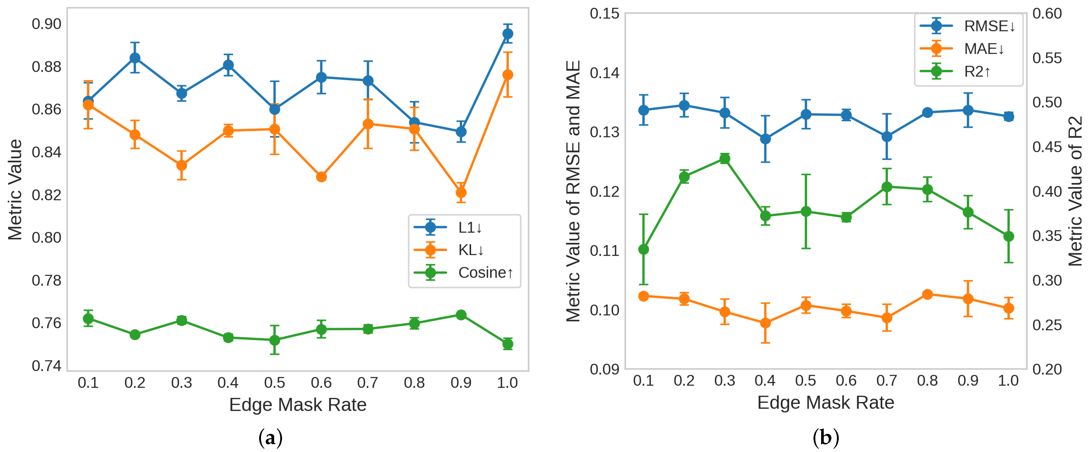
The edge mask rate controls the proportion of edges that are randomly masked in the graph structure during training. As shown in
Figure 4, we conducted experiments with various edge mask rates ranging from 0.1 to 1.0, evaluating the performance of these rates on two downstream tasks: urban functional zone classification (Task 1) and population density prediction (Task 2).
In Task 1, shown in
Figure 4a, lower values are desirable for the L1 error (represented in blue) and KL divergence (orange), while higher values for cosine similarity (green) are preferred. Upon analyzing the results, no distinct trend emerged for these metrics as the edge mask rate varied. However, it can be observed that edge mask rates of 0.3 and 0.9 generally yield relatively good performance across all three metrics, indicating that these rates offer competitive results without significant degradation.
In Task 2, depicted in
Figure 4b, we examined the RMSE (blue), MAE (orange), and
(green) as the evaluation metrics. For the RMSE and MAE, lower values indicate better performance, while higher values of
are preferred. The results reveal an approximately M-shaped trend in performance as the edge mask rate increases. Initially, as the mask rate increases from 0.1 to 0.3, the RMSE and MAE decrease, reaching their optimal values at 0.3. Similarly,
reaches its peak at the 0.3 mask rate, suggesting that a moderate amount of edge masking promotes effective learning. However, at higher mask rates, particularly beyond 0.7, the metrics begin to deteriorate, signaling that excessive masking compromises the structural integrity of the graph, leading to a decline in the model’s performance.
The observed trends indicate that the edge mask rate plays a crucial role in balancing the amount of structural information retained in the graph. While lower mask rates fail to provide sufficient self-supervised learning, higher rates undermine the graph’s structure, which is essential for learning meaningful representations. Thus, after carefully analyzing the results across both tasks, we determined that an edge mask rate of 0.3 strikes an optimal balance. This rate provides a sufficient amount of masking to encourage the self-supervised learning process while maintaining enough structural information for the model to make accurate predictions. Therefore, we selected an edge mask rate of 0.3 as the optimal setting for this study, as it yields competitive performance across all evaluation metrics for both Task 1 and Task 2.
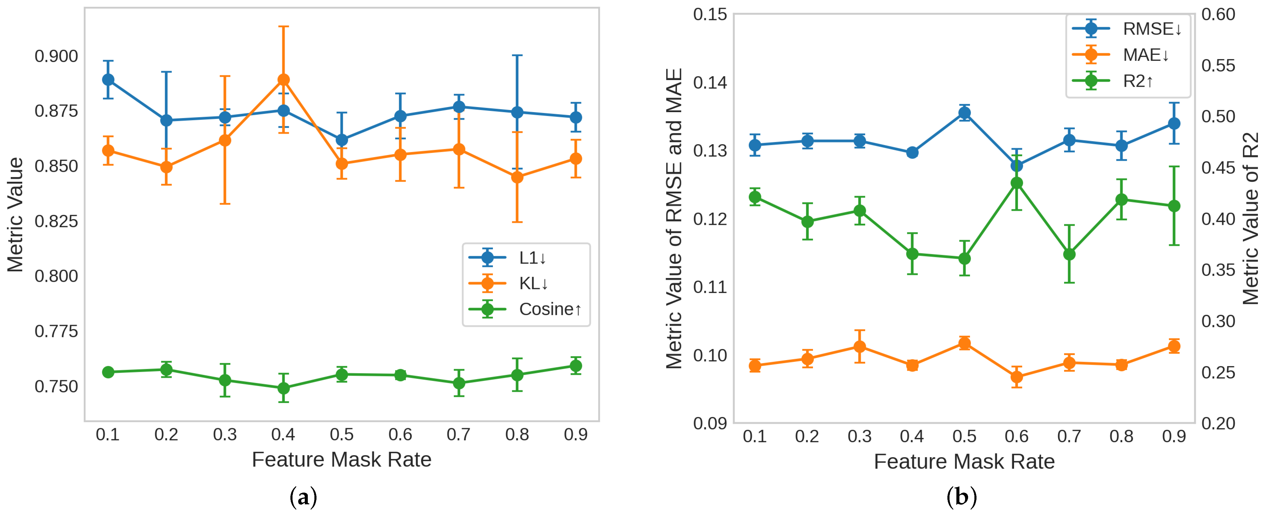
The feature mask rate controls the proportion of node features that are randomly masked during training, thereby influencing the model’s ability to infer missing attributes and learn more robust representations. As shown in
Figure 5, we evaluated the performance of various feature mask rates ranging from 0.1 to 0.9, applying them to both the urban functional zone classification task (Task 1) and the population density prediction task (Task 2).
In Task 1, represented in
Figure 5a, the model achieves a good balance across all metrics around a mask rate of 0.5, with a low L1 error (blue), low KL divergence (orange), and high cosine similarity (green). This suggests that at this rate, the model is effectively encouraged to infer missing node attributes while retaining enough of the feature information to capture the underlying functional relationships in the data.
In Task 2, shown in
Figure 5b, the model achieves its best performance at a feature mask rate of 0.6, where theRMSE (blue) and MAE (orange) are minimized, and
(green) reaches its highest value. This indicates that the model is able to best predict the population density when approximately 60% of the node features are masked. However, when the rate is at 0.5 or 0.7, the model’s performance significantly decreases. In Task 1, the performance at 0.5 and 0.6 is similar.
Based on these findings, a feature mask rate of 0.6 was selected as the optimal setting for this study. Masking around 60% of the node features strikes an effective balance between challenging the model to infer missing information and ensuring that it retains enough input context for accurate predictions. At this rate, the model is exposed to sufficient noise to improve its robustness while still preserving enough of the original feature data to perform well on both tasks. This trade-off makes 0.6 the most suitable choice for optimal model performance in this study.
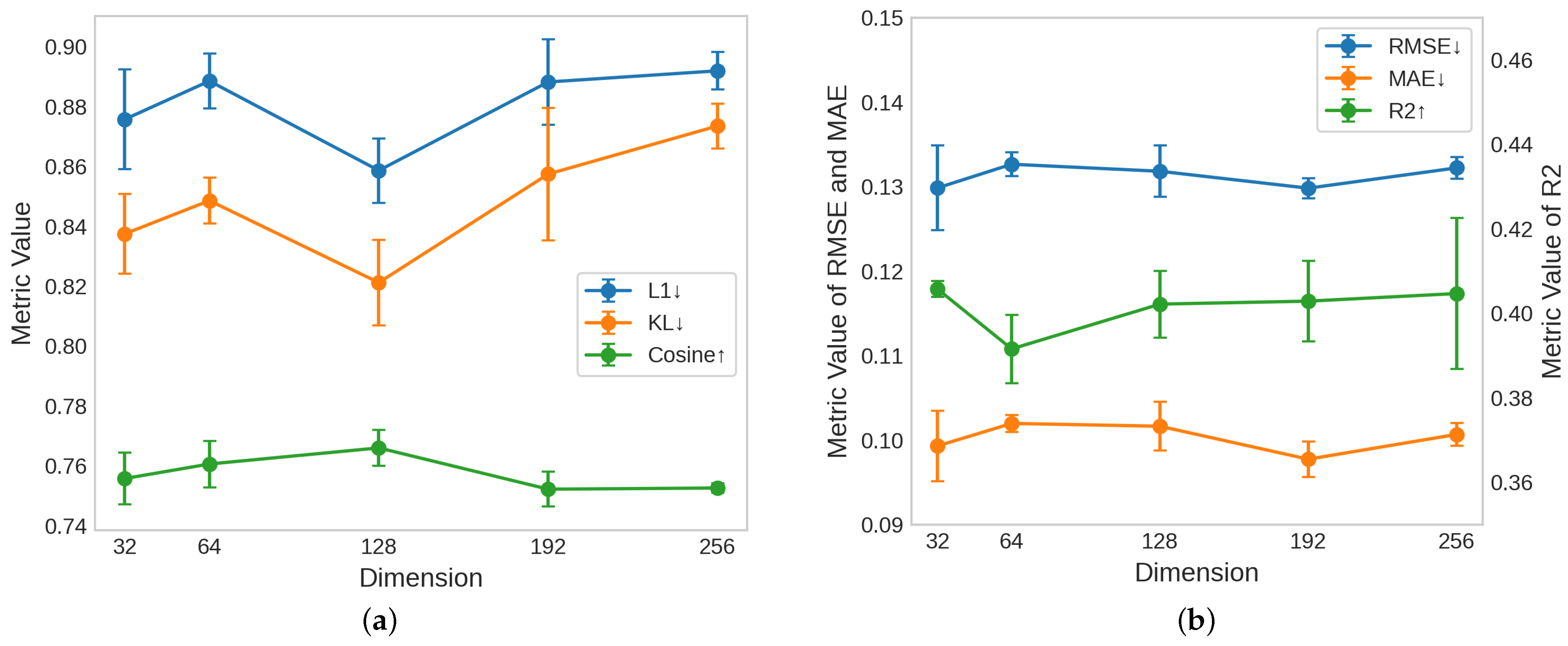
6.2.3. Representation Dimension
The representation dimension represents the size of the learned POI embeddings, which directly affects the expressiveness and capacity of the MaskPOI model. Larger dimensions enable the model to capture more complex relationships and features, while smaller dimensions promote efficiency and may reduce the risk of overfitting. As shown in
Figure 6, we evaluated the impact of different representation dimensions (32, 64, 128, 192, and 256) on both the urban functional zone classification task (Task 1) and the population density prediction task (Task 2).
In Task 1, illustrated in
Figure 6a, the model’s performance initially improves as the representation dimension increases but begins to decline after reaching its peak at 128 dimensions. It clearly shows that 128 is the optimal value for the dimension. In Task 2, shown in
Figure 6b, the model’s performance does not show significant changes with varying dimensions. At a dimension of 64, the model performs noticeably worse, while at 192, the performance is slightly better than at 128. However, in Task 1, the performance at 192 is significantly worse than at 128.
After considering the model’s performance across both tasks, we chose a representation dimension of 128 as the optimal setting for this study. This dimension provides sufficient capacity to capture the underlying relationships in the POI data while maintaining computational efficiency and avoiding the diminishing returns observed at higher dimensions.
6.3. Ablation Study
To evaluate the contributions of the proposed masking strategies in MaskPOI, we conducted ablation experiments by isolating the effects of each component: masking edges (mask edge), masking features (mask feature), and combining both (both). The results are summarized in
Table 4.
The baseline model that incorporates both edge masking and feature masking achieves the best performance across all metrics for both tasks. For urban functional zone classification (Task 1), the baseline model achieves the lowest L1 error (0.867) and KL divergence (0.834) and the highest cosine similarity (0.761). For the population density prediction (Task 2), it achieved the lowest RMSE (0.133) and MAE (0.1) and the highest (0.436). These results demonstrate the complementary benefits of using both masking strategies, which together enable the model to learn robust and comprehensive POI representations.
When comparing the two individual masking strategies, the results indicate that both contribute positively to the overall performance. However, the mask edge strategy provides a more significant improvement compared to the mask feature. For Task 1, the mask edge outperforms the mask feature in all metrics, achieving a lower L1 error (0.884 vs. 0.972), KL divergence (0.884 vs. 0.967), and a higher cosine similarity (0.748 vs. 0.72). Similarly, in Task 2, the mask edge achieves a lower RMSE (0.134 vs. 0.145) and a higher (0.41 vs. 0.324). These results suggest that masking edges has a stronger impact on the model’s ability to capture spatial relationships and structural dependencies, which are crucial for both tasks.
Overall, the results validate the effectiveness of both edge and feature masking, with edge masking providing a more pronounced improvement. The combination of the two strategies yields the best results, highlighting their complementary nature in enhancing the learned POI representations and ensuring robust performance across tasks.
7. Discussion
In this section, we explore how the construction of the POI graph and the initial feature embedding affect POI representation, and we also discuss the limitations of MaskPOI.
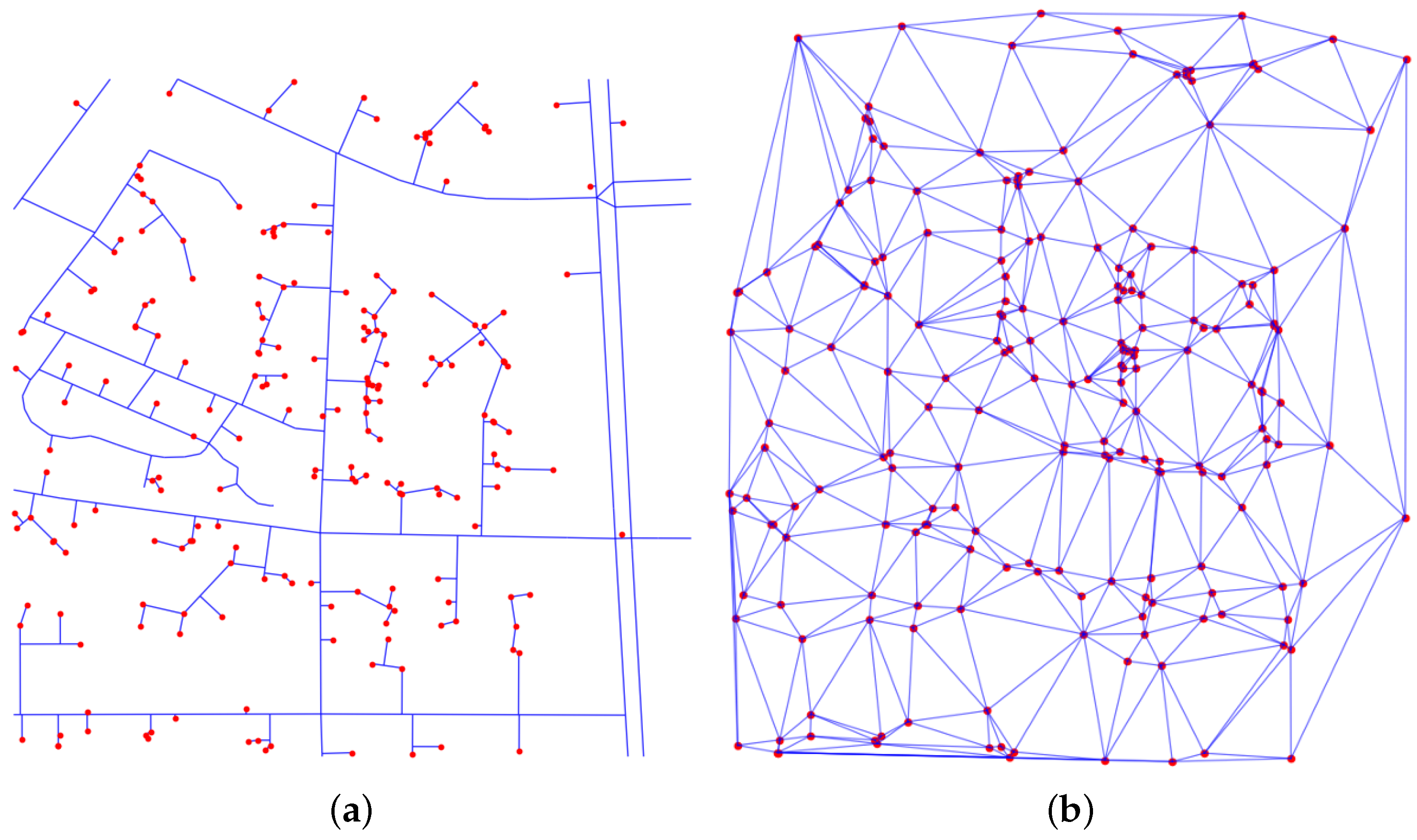
7.1. Impact of Graph Construction Method
In this study, we constructed the network by connecting POIs to their nearest roads, creating a hybrid road+POI network that captures both the spatial relationships among POIs and their alignment with the road network. To further evaluate the impact of the network construction methods, we compared this baseline approach with a purely POI-based method using Delaunay triangulation to construct the network. The differences between the two methods of constructing networks for the same POI data are shown in
Figure 7.
The comparison is presented in
Table 5. The results show that the two network construction methods yield similar performances across both tasks. One possible reason for the similar performance between the two network construction methods is that both approaches effectively capture the essential spatial relationships between POIs, which are crucial for the downstream tasks. Although the hybrid road+POI network explicitly incorporates road information, the Delaunay triangulation method also creates a graph structure that closely reflects the spatial distribution of POIs. As a result, both networks provide meaningful topological information that supports the representation learning process.
Another contributing factor might be the robustness of the representation learning framework employed in this study. The use of mask-based modeling enables the discovery of implicit information, such as latent spatial relationships that are not explicitly represented. Consequently, despite the structural differences between the two graphs, the network is capable of learning and capturing the same implicit relationships.
7.2. Impact of Initial POI Feature Embedding
In this study, we utilized BERT [
28] to construct the initial features for POIs, capturing semantic information from their textual descriptions. To analyze the impact of different text encoding methods, we compared the BERT-based embedding approach with a one-hot encoding method.
One-hot encoding is a conventional approach for categorical data representation, where each unique category is mapped to a high-dimensional sparse binary vector. In our case, POIs are categorized using a three-level hierarchical structure. To construct one-hot encoded representations, we follow these steps:
Category Indexing: Each level of the POI hierarchy is assigned a unique index within its respective level.
Binary Vector Representation: Each POI is represented using three separate one-hot vectors, one for each category level. The vector has a length equal to the total number of unique categories at that level, with a single “1” at the corresponding index and all other positions set to “0”.
Concatenation: The three one-hot vectors corresponding to the three levels are concatenated to form the final one-hot representation.
The results, presented in
Table 6, demonstrate the performance differences between BERT embeddings and one-hot encoding. To assess whether these improvements are statistically significant, we conducted a paired
t-test for each metric. Statistically significant differences (
) are indicated with an asterisk (*).
For urban functional zone classification, BERT-based embeddings outperform one-hot encoding across all metrics, but the improvements seen in the L1 error () and KL divergence () are not statistically significant. However, the improvement in cosine similarity () is significant, suggesting that the BERT embeddings better capture the semantic relationships within POI categories.
For population density prediction, the BERT embeddings demonstrate statistically significant improvements across all metrics (), including the RMSE (), MAE (), and (). These results confirm that the richer semantic representations provided by the BERT embeddings lead to more accurate population estimations.
Overall, these findings validate the choice of BERT embeddings in this study, as they not only enhanced the model’s performance but also introduced greater semantic expressiveness and robustness, particularly in tasks that require a fine-grained understanding of POI relationships. While certain improvements did not reach statistical significance, the consistent trend suggests that the BERT embeddings provide a more informative representation than one-hot encoding, reducing our reliance on manually defined category hierarchies.
7.3. Limitations
MaskPOI presents certain limitations that should be addressed in future research. First, the high dimensionality of the POI feature encoding (2306 dimensions) significantly increases memory consumption. This makes it challenging to construct large graphs, especially when we attempt to capture relationships over extended spatial distances. In this study, we constructed graphs within a 500 m region, but to better capture long-range spatial dependencies, larger graphs would be needed, which, in turn, require more efficient processing techniques. Future work could explore methods for dimensionality reduction or more efficient graph processing algorithms that can handle larger, high-dimensional graphs, allowing for the construction of graphs over broader areas or longer distances.
Second, the POI features used in this study are limited to coordinates and category labels, which provide only a basic representation of each POI. However, POIs typically contain other valuable attributes, such as names, user reviews, ratings, and other metadata, which could significantly enhance the expressiveness of the POI features. Integrating these additional data sources could provide a richer feature set, improving the model’s ability to capture the full spectrum of POI characteristics. Future research should focus on incorporating multi-modal information to create more comprehensive representations of POIs, potentially improving the performance of the MaskPOI framework in various tasks.


