A Terrain Classification Method for Quadruped Robots with Proprioception

Abstract

Acquiring terrain information during robot locomotion is essential for autonomous navigation, gait selection, and trajectory planning. Quadruped robots, due to their biomimetic structures, demonstrate enhanced traversability over complex terrains compared to other robotic platforms. Furthermore, the internal sensors of quadruped robots acquire rich terrain-related data during locomotion across diverse terrains. This study investigates the relationship between terrain characteristics and quadruped robots based on proprioception sensor data, and proposes a simple, efficient, and motion-independent terrain classification method by integrating multiple sensor signals. The sensors referred to in the text only include the IMU sensor and joint encoders, which means that the method has a wide range of applicability while requiring sufficiently low hardware cost. The Convolutional Neural Network will serve as the backbone of the algorithm. In addition, the control command about its own control information will serve as supporting information to eliminate the impact of motion patterns on the results. Employing a multi-label classification algorithm, the complex terrains are classified by multiple physical feature labels like roughness, slippage, softness, and slope, which depict terrain attributes. A feature-labeled terrain dataset is established by abstracting diverse terrain features across various terrains. Unlike semantic labels (e.g., grassland, sand, gravel) that are comprehensible only to humans, feature labels provide a more helpful and precise terrain characterization, including broader terrain attributes.

1. Introduction

It has always been a primary aim for robotic researchers to enable robots to navigate and traverse various complex, and even hostile, terrains successfully. With this objective, the ability to detect corresponding complex and hazardous terrains and either avoid them or adjust the motion strategy accordingly is an indispensable capability for future intelligent robots. To achieve more robust perceptual outcomes, the integration of data from diverse sensors to obtain multidimensional and complementary perceptual information, aiding robots in decision-making, is an anticipated trend for the future.

Compared with vision-based terrain classification, which has been widely studied, proprioceptive sensing offers advantages in scenarios where vision may be unreliable, such as low-light, foggy, or visually occluded environments. Additionally, proprioceptive sensors provide direct physical interaction feedback, enabling more accurate assessments of terrain properties like stiffness, slipperiness, and compliance, which are crucial for safe locomotion. While vision-based methods offer rich environmental context, they often require complex algorithms for interpretation and can be affected by environmental conditions.

Currently, the methods employed for environmental perception can be broadly categorized based on exteroceptive sensors and proprioceptive sensors [1,2]. Exteroceptive-sensor-based terrain perception methods include LiDAR-based [3,4], camera-based [5,6,7,8], and sound-based [9,10,11,12] techniques. Methods based on external sensors enable non-contact advance judgments and predictions of terrain, transmitting perception results to the controller for corresponding strategy adjustments without physically interacting with complex terrains. Sound-based terrain perception methods capture sound signals using microphones installed on the robot’s body, processing them to derive terrain-related feature information. The methods based on proprioception for terrain feature perception often do not directly acquire environmental information but instead infer changes in the terrain by monitoring variations in the robot’s own state. Precisely because proprioception-based perception methods acquire terrain features indirectly, methods relying on a single proprioceptive sensor often have limited effectiveness. Therefore, many studies focus on multi-sensor fusion to enhance the performance of such methods [13,14,15].

Another type of proprioceptive sensor is contact-based [16,17], such as force sensors or touch sensors installed at the robot’s foot-end. Due to direct ground contact, the information acquired by these sensors is closely related to ground conditions, providing intuitive reflections of the robot’s motion state changes and yielding satisfactory results.

To date, a considerable number of researchers have attempted to use proprioceptive perception to judge and classify the current terrain of robots. As early as 2004, Karl Iagnemma et al. [18] introduced MIT’s vibration-signal-based terrain perception method for rovers. They collected terrain vibration signals from sensors located on the vehicle body and processed matrices with frequency domain information collected from different terrains to obtain a measure that can distinguish terrain. Mario Calandra et al. [19] proposed a methodology based on reservoir computing for obtaining terrain information and ground reaction forces from proprioceptive information acquired at the level of the leg joints of a simulated quadruped robot.

Kai Zhao, Mingming Dong, and Liang Gu et al. [11] used noise signals, body vibration signals, and the vibration signal of the first wheel as inputs. They established a multi-model fusion classification algorithm to classify each input and fuse the results to obtain the final terrain classification result. Brooks and Iagnemma [20] proposed a self-supervised terrain classification method that effectively combines visual sensor information with vibration information. Chengchao Bai and Jifeng Guo et al. [2] proposed a terrain classification method based on multi-layer perceptrons. The authors preprocessed and converted the spectrogram signals of the body’s three-axis acceleration into a multidimensional vector, which was then used as input to train the multi-layer perceptrons.

The above methods are mostly learning algorithms that require manual feature design. After the advent of CNNs, manual feature extraction still holds value, but automatic feature extraction has gradually become the mainstream approach. Angelo Ugenti et al. used the time–frequency graph method to represent the obtained robot vibration data and torque data and tested the accuracy of terrain recognition using a CNN and SVM, respectively. Among them, the CNN measured the highest accuracy, with an average accuracy of 96% [1]. Junlong Guo and Xingyang Zhang et al. used a purely visual approach to classify public terrain datasets using a lightweight convolutional neural network (YOLOv5), with a classification accuracy of around 90% [21]. Fabio Vulpi and Annalisa Milella et al. used a combination of a CNN and RNN for terrain classification. They first converted the time-domain signals of IMU and motor over a period of time into time–frequency maps and compared the model performance of CNN, RNN, and LSTM networks. The results showed that the CNN had the best performance, and compared to temporal models, convolutional neural networks were obviously easier to train [3].

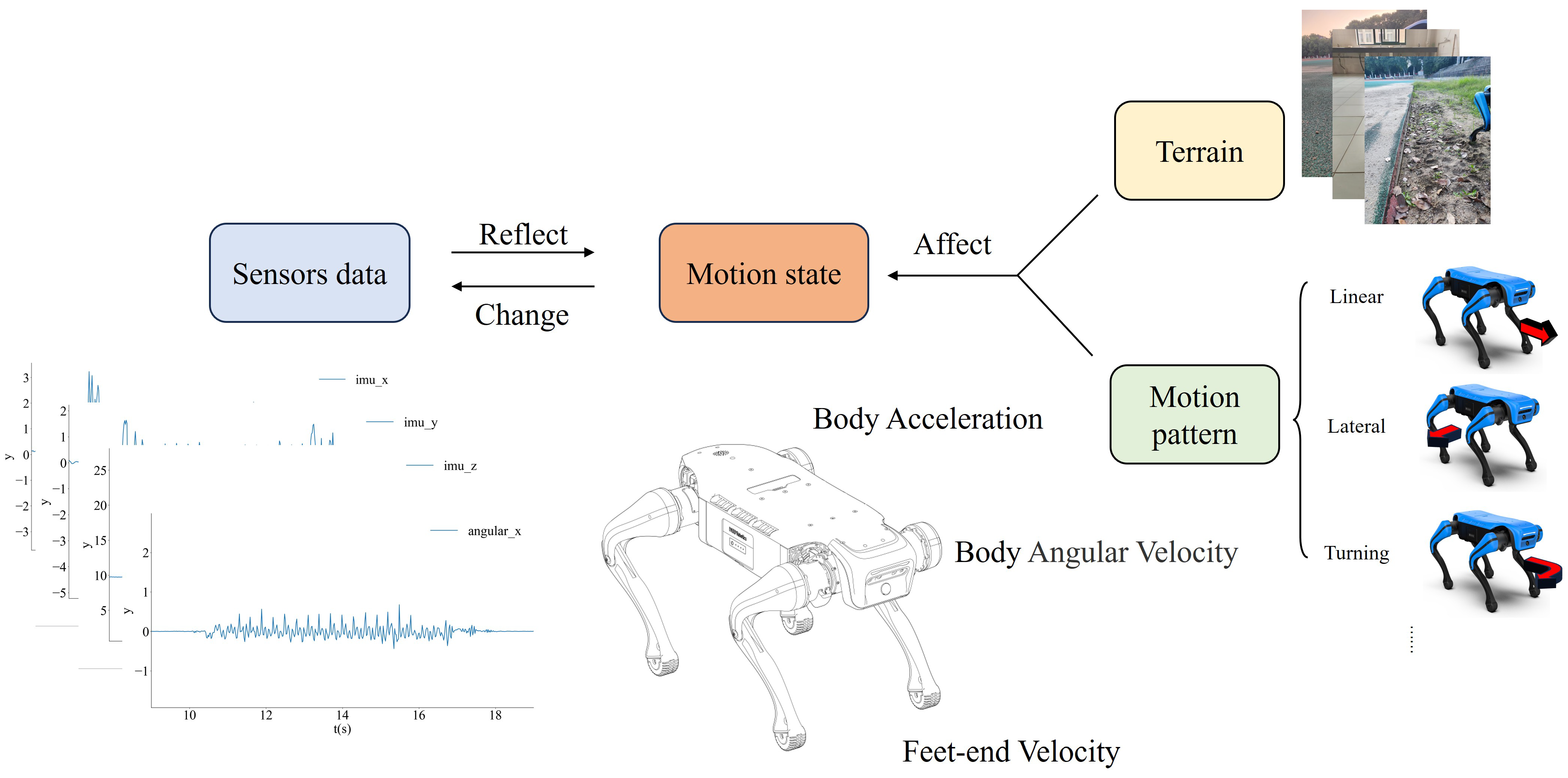
This paper proposes a multi-sensor fusion algorithm based on convolutional networks used to extract the features of each sensor signal. In addition, a terrain characteristic classification method is introduced. Complex terrains are abstracted into multi-physical combination labels, including roughness, slippage, softness, and slope. During this process, the model learns the robot’s motion information through both explicit and implicit means. In addition, a multi-sensor signal heatmap, which is an efficient way to integrate information from multiple sensors into a single image, is introduced. Finally, the command instruction vector provides supporting information and is concatenated to eliminate the influence of the robot’s own motion pattern caused by control commands. The relationship between sensor data, motion patterns, and motion states is illustrated in Figure 1.

The rest of this paper is organized as follows: Section 2 presents the details of the proposed approach, and Section 3 introduces the experimental setup. The results and analysis are given in Section 4. Finally, Section 5 concludes this paper.

2. Methodology

2.1. Hypothesis

The main focus of this study is to integrate the proprioceptive perception signals of quadruped robots. Therefore, the required input data includes IMU vibration data along the x-, y-, and z-axes; angular velocity data along the x-, y-, and z-axes; and the relative foot-end velocity to the body along the x-, y-, and z-axes. The reason for choosing these data is that the IMU vibration and angular velocity data along the x-, y-, and z-axes can reflect the degree of roughness, slope, and softness of the ground. Additionally, the relationship between the relative foot-end velocity and IMU vibration data can reflect the degree of slippage. Furthermore, the command instructions, which include x-, y-, and z-axis angular velocity commands and linear velocity commands, represent the robot’s partial motion patterns and help the model understand the impact of its own motion on the sensor data. However, in addition to the motion state changes caused by its motion velocity and direction, the gait pattern of a quadruped robot can also change the robot’s motion state, affecting the feature distribution and structure of the sensor data. Therefore, the impact of motion state is mitigated by using multiple sets of training data with different gaits, allowing the algorithm to implicitly learn the relationship between gaits and terrain.

When the influence of the motion state caused by its own command, which we refer to as the motion pattern, is eliminated, ideally, the only factor that can cause changes in the sensors is terrain variation. If terrain information is represented as n and the motion state as T, the feature space of the ground information n is $[{\mathrm{n}}_1,{\mathrm{n}}_2,{\mathrm{n}}_3,\dots ,{\mathrm{n}}_{\mathrm{n}}]$, where ${\mathrm{n}}_{\mathrm{i}}$ represents a specific ground state, such as roughness, slippage, softness, or slope. Then, the relationship between the two can be expressed as:

$$f\left(n\right)=T$$

(1)

In Equation (1), f(·) represents the functional relationship between the terrain and the robot’s motion state. It is a nonlinear function that captures how changes in terrain lead to changes in the robot’s motion state. This function is influenced by various factors, such as the robot’s materials, structure, and control strategies. When we attempt to characterize the motion state using data from multiple sensors, denoted as ${\mathrm{x}}_{\mathrm{i}}$, the equation should be:

$$g(x_1,x_2,\dots ,x_n)=T$$

(2)

In Equation (2), g(·) represents the mapping relationship between the multi-sensor input information and the robot’s motion state. The relationship between these two may be a more complex nonlinear function. Thus, based on Equations (1) and (2), we can derive the equation for terrain information with multi-sensor data as the independent variables:

$$f^{-1}\left[g(x_1,x_2,\dots ,x_n)\right]=n$$

(3)

Therefore, based on Equation (3), constructing a multi-sensor fusion deep learning algorithm is essentially building the function: ${\mathbf{f}}^{-\mathbf{1}}\circ \mathbf{g}$. Additionally, based on the definition of the function, input ${\mathbf{x}}_{\mathbf{i}}$ at a certain moment or over a period of time corresponds to, and only corresponds to, one type of terrain n. This is because if the same sensor measurement values appear for different terrain states, i.e., a multi-valued mapping relationship, it would go beyond the scope of the nonlinear function established in this study based on deep learning. This is indeed a strong assumption. As shown in Figure 2, The images display some signal features recorded during linear motion. It is evident that the angular velocity waveform becomes irregular on uneven terrain, compared to its behavior on even terrain. In slippery terrain, the sudden change in foot speed and the mismatch with the robot’s torso acceleration create abnormal features for this label. In soft terrain, the magnitude variation range of the z-axis acceleration signal distribution is larger. In sloped terrain, the mean of the vibration signal on the x-axis shifts. Waveform diagrams reveal unique data features in certain terrains, while also illustrating the data distribution of the most significant sensor variations across different terrains.

2.2. Overview

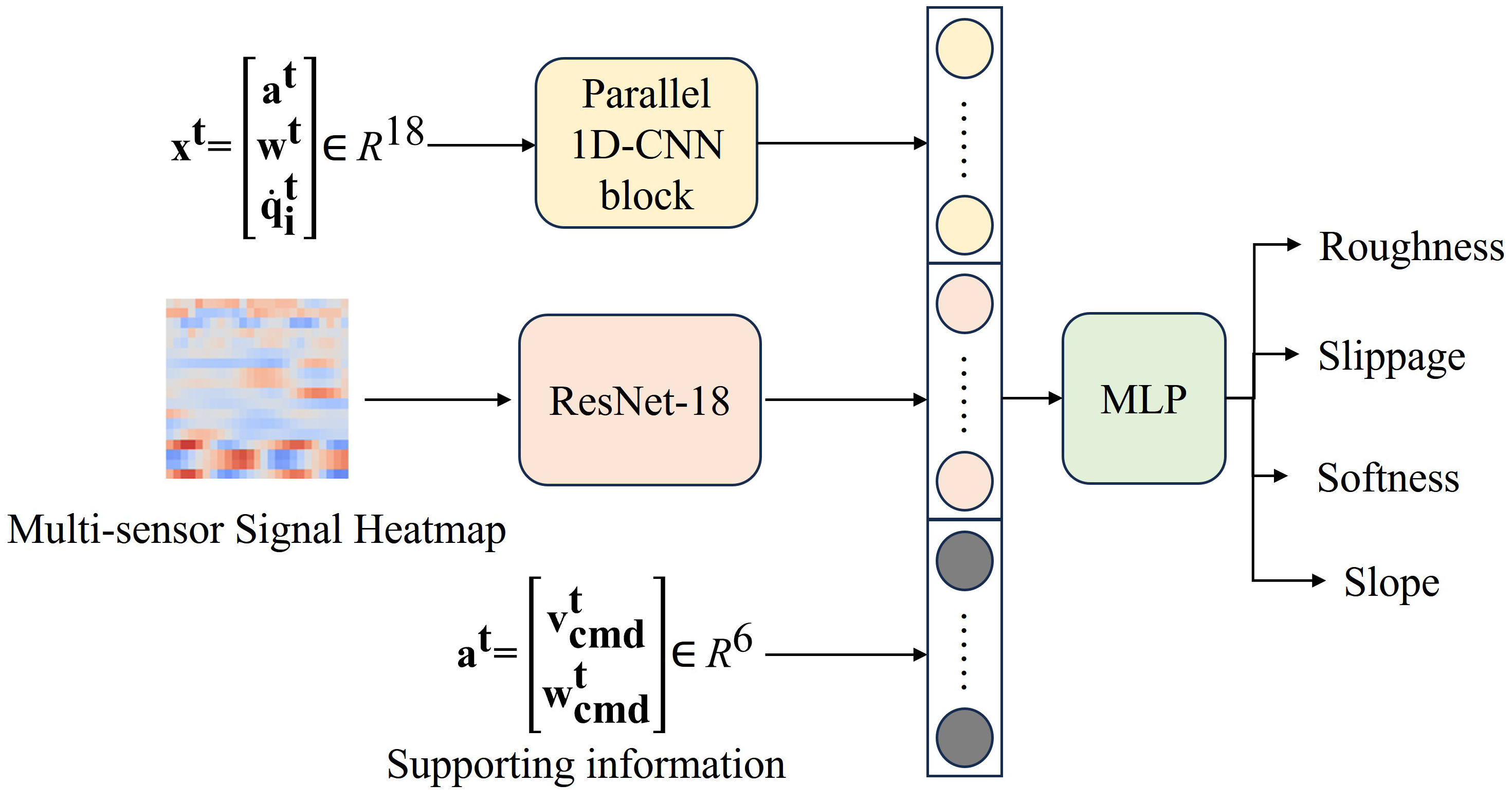
As shown in Figure 3, the structure of the entire network can be divided into three main parts: the time-dependent feature branch, the heatmap feature branch, and the supporting information branch. First, the time-dependent feature branch consists of parallel 1D-CNN blocks marked in yellow in Figure 3. The input ${\mathbf{x}}^{\mathbf{t}}$ of this branch consists of three-axis acceleration, three-axis angular velocity, and three-axis foot-end velocity. 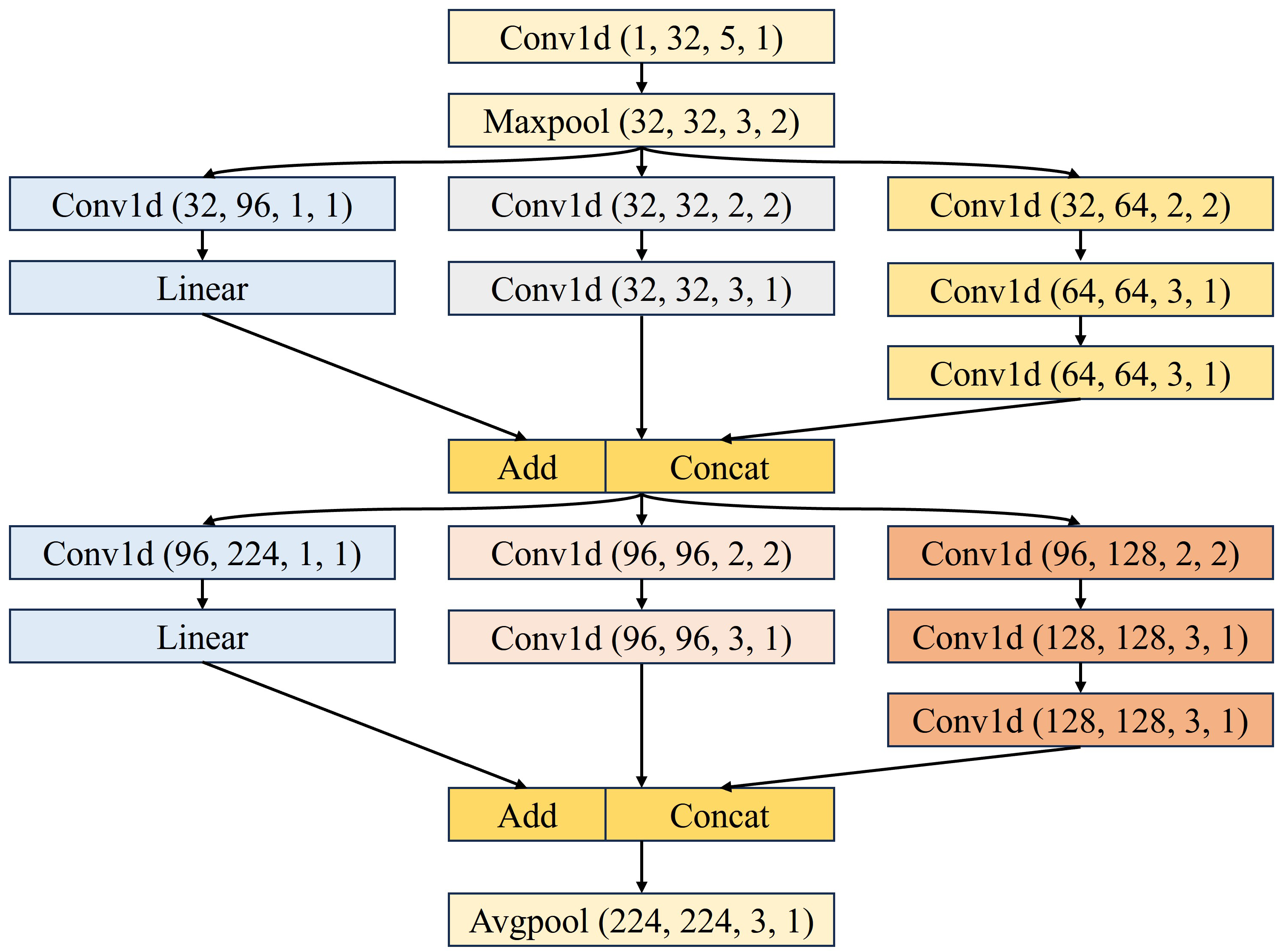The superscript $\mathbf{t}$ represents the sample points over a period of time at a certain sampling frequency, meaning the input is a list containing 18 sensor data tensors., and each 1D-CNN channel is composed of a series of 1D convolution networks as shown in Figure 4, with each parallel convolution channel processing corresponding signals.

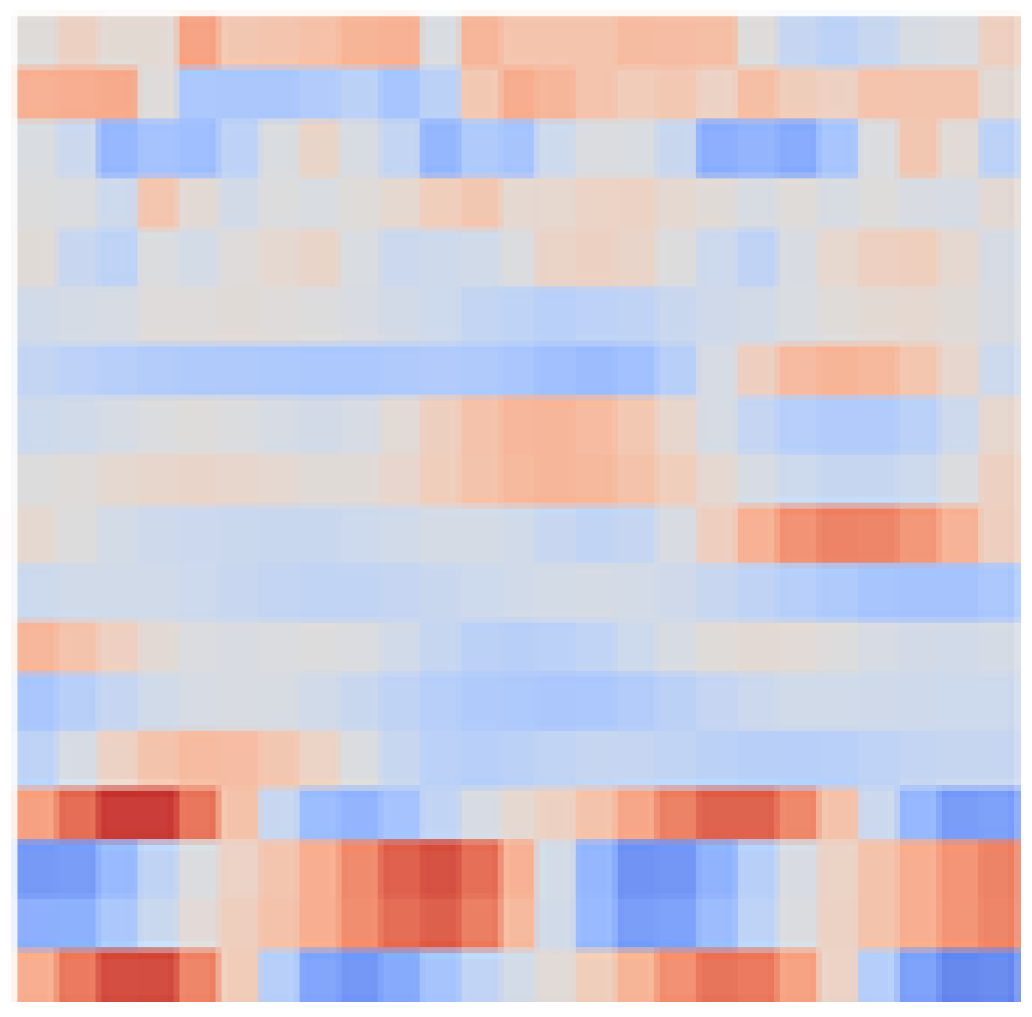
Second, the heatmap feature branch consists of an image recognition model in pink in Figure 3, designed to capture the features of the heatmap image. Each row includes the values of a sensor over a period of time, with all values normalized to the same range. Therefore, these values can be visualized on a single image with a consistent color scale.

Third, the supporting information branch consists of the commanded linear velocity along three axes and the commanded angular velocity along three axes. This branch provides part of the motion pattern information caused by its own control command to make the model unaffected by this part. The other part, which exhibits changes in its motion patterns, is implicitly learned by the model through training on the data with diverse motion patterns.

2.3. Time-Dependent Feature Branch

In time-dependent feature branch, each 1D convolutional tunnel processes a single sensor signal. It is designed to capture dependencies of temporal signal using multiple convolutional kernels of different sizes, which is similar to inception module. The 1D-CNN structure of a single tunnel is shown in Figure 4. The shape of the input tensor is batch × 1 × 25, where 25 represents the number of sample points. As shown in Figure 4, the convolutional network contains branches with convolutional kernels of different sizes to capture temporal dependencies at different scales. The final size of the vector of the 1D-CNN block is 4032, with each tunnel’s vector of size 224 concatenated. There is a BN layer and a ReLU layer following each convolutional layer. When the feature map sizes do not match, a linear layer would be added for dimensional adjustment.

2.4. Heatmap Feature Branch

In the heatmap feature branch, a pre-trained ResNet is used as the backbone instead of retraining an image classification network as the backbone because ResNet has been proven to perform excellently in image classification tasks, and its superior pre-trained parameters allow the model to be used with minimal adjustments. Using a CNN trained from scratch is indeed an optimization for future work, but in the case where the effectiveness of multi-sensor fusion methods is uncertain, using a network with unknown performance in classification tasks would significantly increase the workload.

ResNet-18 is a deep convolutional neural network famous for image classification within the Residual Network family. Authors resolved the degradation problem of deep convolutional neural networks by introducing residual connections, with “18” indicating the network’s depth of 18 layers. ResNet is composed of multiple stages, each consisting of several residual blocks. The feature map’s channel dimensions only change when feature map size is changed to preserve the time complexity. The basic structure of the residual block is shown in Figure 5 and consists of a 3 × 3 convolutional layer, a BN layer, and ReLU. Due to computational constraints at the time, two 1 × 1 convolutional layers were added to the basic residual block, forming the Bottleneck residual block. This design reduces the channel dimensions of the feature map before increasing them again, reducing intermediate computation costs. The reason for using ResNet-18 as the backbone is that compared to deeper variants of ResNet (ResNet-34, ResNet-50, ResNet-101, ResNet-152), its performance in the fusion model does not significantly improve. However, as the network deepens, the number of parameters that need to be trained increases exponentially.

In the heatmap feature branch, the input is a heatmap image of multi-sensor signals, forming RGB images with dimensions of 3 × 224 × 224 in tensor format. The heatmap represents the values of multi-sensor signals after normalization, with the columns corresponding to the time axis of the sensor data. Specifically, each rectangular color block on the y-axis of the heatmap represents, from top to bottom, x-, y-, and z-axis acceleration; x-, y-, and z-axis angular velocity; and x, y, and z foot-end velocity, totaling 18 rows. The x-axis represents the time axis, with a total of 25 time points. Using the heatmap as input not only allows for the extraction of temporal features from each signal but also enables the capture of dependencies between different signals due to the nature of 2D convolution. Using the heatmap as input not only allows for the extraction of temporal features from each signal but also enables the capture of dependencies between different signals due to the nature of 2D convolution. Additionally, a part of the motion pattern information is reflected in the heatmap. As shown in Figure 6, when the quadruped robot walks in a straight line, the last four rows of the heatmap resemble the gait planning of the robot, and these last four rows correspond exactly to the robot’s foot speed in the x-direction (forward and backward direction).

2.5. Supporting Information Branch

The supporting information branch provides information about motion patterns from control commands and helps the model distinguish whether changes in sensor signals are due to terrain or control commands. Moreover, the correlation between control commands and signals from sensors, such as control velocity and foot-end velocity or control angular velocity and body angular velocity, helps develop new features for terrain classification.

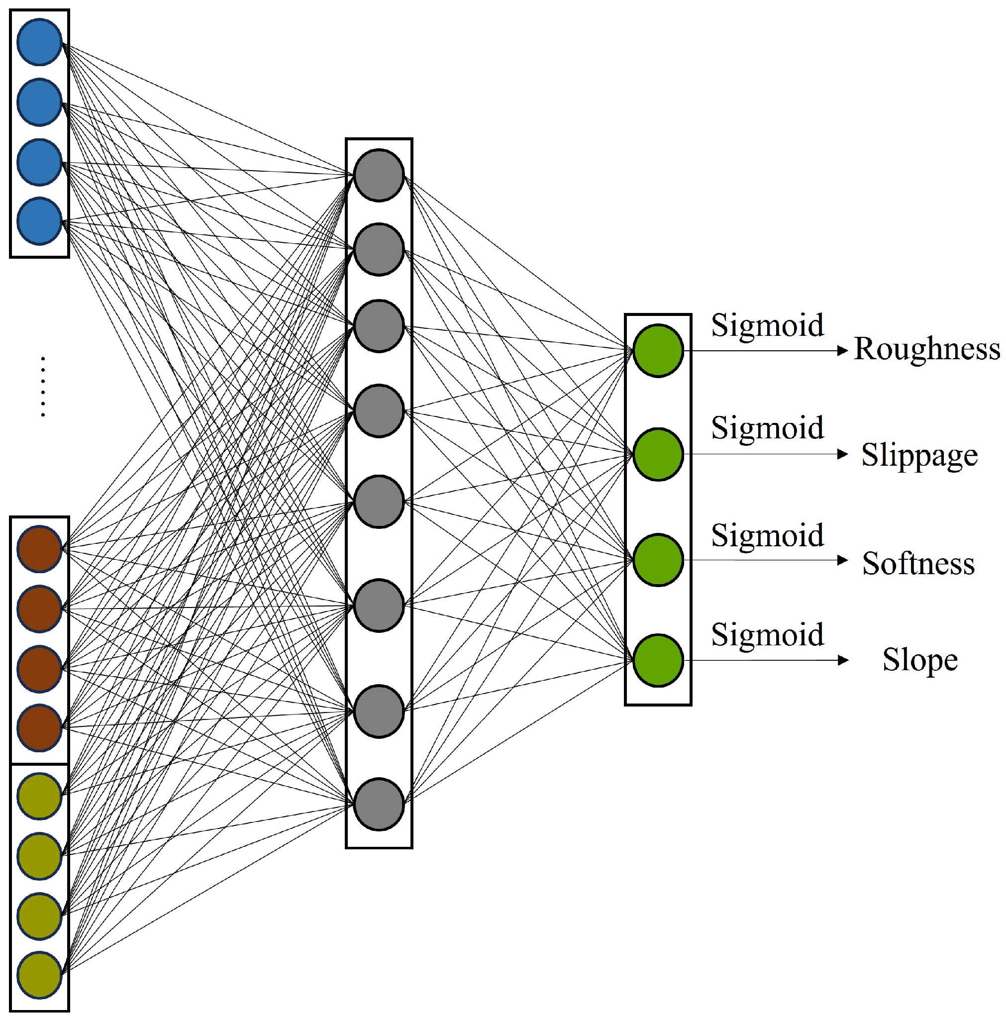
2.6. Multi-Label Classifier

The multi-label classifier is composed of a fully connected network, with its specific structure illustrated in Figure 7. Its purpose is to reduce multi-dimensional vectors containing both feature and relational feature information and then output the classification results for each label through a sigmoid activation function. The network parameters are updated using binary cross-entropy as the loss function. However, instead of the common approach where the loss for each label is summed or weighted and backpropagation is performed over each episode or batch, this paper adopts a method where each label head performs a separate forward inference and backpropagation process within an episode. This means the network is updated four times in one episode. The loss function for a specific label can be expressed as:

$$Los{s}_i=-{\displaystyle \frac{1}{n}}\sum _{j=1}^n{y}_j^{*}log\left(y_j\right)$$

(4)

In Equation (4), y represents the predicted value, y* is label value, j denotes the j-th training sample in the training set, and i is the i-th label head. The binary cross-entropy loss function is backpropagated separately for each label within an episode, meaning that a batch of data is utilized multiple times, thereby increasing data usage efficiency. Moreover, this approach prevents the algorithm from using the loss of one label head with a larger loss to train another label head that already performs well. The comparison chart of training using the traditional backpropagation strategy, and the new backpropagation strategy is shown in Figure 8. Figure 8a shows the loss and accuracy changes on the validation set for a model where four label heads perform backpropagation separately within a single batch. Since both the loss and precision values range from 0 to 1, they share the same axis. It is clearly observed that the accuracy and loss of the four label heads stabilize around episode 400. In Figure 8b, the accuracy and loss changes using the traditional backpropagation strategy are shown. It can be observed that on the same dataset, the model has not yet reached a convergent state.

3. Experimental Setup

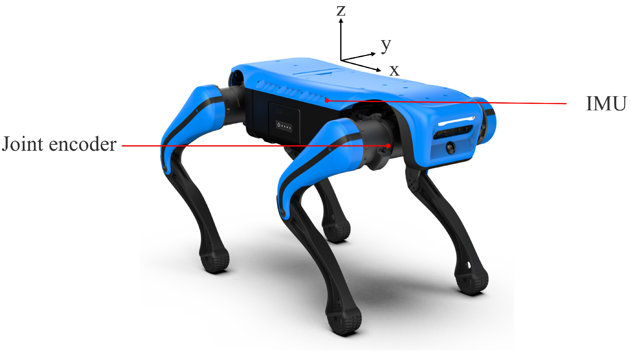
The quadruped robot platform used in this study is a product of Hangzhou Yunshenchu Technology Co. Ltd., Hangzhou, China named “JueYing Lite2 Professional Edition”. JueYing Lite2 Professional Edition is a versatile intelligent quadruped robot with 12 degrees of freedom and various motion gaits. The robot stands 355 mm tall, measures 540 mm in length from head to tail, 315 mm in width, and weighs 10 kg. The sensors used in the experiment include: IMU and joint encoder sensors. The placement of these sensors on the robot is illustrated in Figure 9.

3.1. Dataset

In this study, all experimental data were obtained through the IMU sensor and joint encoder carried by the JueYing Lite2 quadruped robot. Specifically, the data consist of the IMU’s x-, y-, and z-axis vibration data; body angular velocity data around the x-, y-, and z-axes; and the foot-end relative x-, y-, and z-axis linear velocity data, which were obtained through forward kinematics and joint angle calculations.

The body vibration data and body angular velocity data are from the IMU sensor, while the foot-end velocity data are from the joint encoder. The sampling frequency of both the IMU and joint encoder is 50 Hz. However, due to the instability of the sampling frequency, there is a different number of data points from different sensors. To maintain consistency in data quantity and sampling frequency across different sensors, interpolation methods were employed. Specifically, linear interpolation was applied to the body vibration data, body angular velocity data, and foot-end velocity. Additionally, due to sensor errors, the raw time-domain data contain many sudden “spikes” in the joint encoder, which can produce large abrupt values during differentiation. On the one hand, the sensors used in this experiment are of low cost, with a nominal sampling frequency of only 50 Hz, and the actual sampling frequency during testing is even lower. This leads to distortion in the joint angle measurements, even under good terrain conditions. On the other hand, actuator jitter over short periods of time also causes spikes in the measurement data. In this case, a low-pass filter had to be used to remove these spikes without damaging the original data distribution. Finally, the uniformly sampled time-domain data were windowed, with each window containing 25 data points, representing a waveform of 0.5 s duration with a stride of 5 data points. The windowed time-domain data in the training set were globally normalized to obtain normalized parameters for training, validation, and testing.

It is important to note that this study directly used time-domain data as samples without performing Fourier transforms or other frequency-domain operations to introduce frequency-domain information. This is because, in this study, the temporal information is important for capturing the correlation between the signal and terrain. Applying Fourier transforms or other frequency-domain operations would lead to the loss of temporal information.

As shown in

Table 1. Distribution of dataset.

Labels				Training	Validation	Test
Roughness	Slippage	Softness	Slope
0	0	0	0	2426	221	236
1	0	0	0	2472	245	201
X	1	X	X	2424	238	239
0	0	1	0	2489	225	333
0	0	0	1	2463	239	253

, a value of the label “roughness” closer to 0 indicates a flatter terrain, while a value further from 0 indicates rougher terrain. A value of the label “slippage” closer to 0 means the terrain has less slippage, while a value further from 0 indicates more slippage. A value of the label “softness” closer to 0 means the ground is harder, while a value further from 0 indicates softer ground. A value of the label “slope” closer to 0 means the slope is steeper, while a value further from 0 indicates the ground is closer to being flat. The closer each label is to 0, the better the ground condition. The labels 0 and 1 are determined by a threshold of 0.5.

The physical terrain characteristic labels were subjectively assigned. Considering the instability of subjective labeling, we used terrains with distinctly dominant features, such as concrete pavement, sand, and grass, to assign labels and minimize errors caused by subjective labeling. This is also why we designed the label distribution in the training set by gradually altering one characteristic at a time.

The flat terrain with the “0000” label represents the optimal condition terrain. The uneven terrain with the “1000” label represents rough terrain but with optimal conditions in other terrain characteristics. The slippage terrain with the “X1XX” label represents the snowy terrain or sandy terrain. In “X1XX” label, “X” represents the uncertainty about terrain characteristics because of the fluidity of snow and sand terrain. Due to the particularities of snowy and sandy terrain, it is difficult to precisely define the roughness and slope of fluid terrain based on personal judgment. However, there are common characteristics of terrains with fluid properties like slippage and softness. Due to weather and humidity factors, the hardness on snowy and sandy terrains is not even during the experiment. To be cautious, only slippage was used as the definitive label. During the training process, the masked labels output the forward propagation results but did not participate in the backpropagation process. During the validation and testing phases, the masked labels output inference results, but their results were not included in the statistical results. Therefore, in this study, the label X is neither 0 nor 1, indicating an uncertain ground condition. The soft terrain with the “0010” label represents grass terrain and soft carpet terrain. The slope terrain with the “0001” label represents slope terrain but with optimal conditions in other terrain characteristics. Specific dataset information is provided in Table 1.

The terrain conditions involved in this study include the following:

(1)

Sensor signals from an ideal flat terrain form the “0000” label dataset, like solid concrete terrain and plastic terrain, as shown in Figure 10a,b.

(2)

Sensor signals from a slippery terrain form the “X1XX” label dataset, like snowy terrain and sandy terrain, as shown in Figure 10c,d.

(3)

Sensor signals from a flat slope form the “0001” label dataset, like slope terrain, as shown in Figure 10e.

(4)

Sensor signals from an uneven terrain form the “1000” label dataset, like uneven brick terrain, as shown in Figure 10f.

(5)

Sensor signals from a soft terrain form the “0010” dataset, like soft grassy and soft carpet terrain, as presented in Figure 10g,h.

3.2. Experimental Details

Min-max normalization was applied to the data of each sensor, which means that for each sensor’s data, there is a corresponding minimum and maximum value parameter, which were then applied to the validation and test sets. The optimizer used during training is the Adam optimizer, with an initial learning rate of 1 × 10⁻⁵. The batch size is 25. The parameters in the ResNet-18 model adopted in this study were downloaded from pre-trained weights. It was observed that models with ResNet as the backbone converge quite rapidly, achieving satisfactory model performance after just one epoch. The model threshold was set at 0.5.

3.3. Comparing Experiments

In the comparative experiment, multiple backbones were used to contrast the performance, including the following: (1) Variants of ResNet [22] (ResNet-18, ResNet-34, ResNet-50); (2) Variants of Inception [23] (Inception V4); and (3) Transformer [24], where multiple sensor inputs at each time step form a vector and multiple time steps constitute the input for Transformer. Utilizing Transformer as the backbone essentially transforms the sensor fusion classification task into a temporal task.

In addition to the backbones, experiments were also designed with several excellent multi-sensor fusion algorithms, including the following: (1) Proprioception Net [25]: Proprioception Net processes and classifies two-dimensional vectors composed of multiple sensor information through multiple one-dimensional convolutional layers. Essentially, it converts the multi-sensor fusion classification task into a time-series problem; (2) MLP [26]: MLP is a low-resource online terrain classification algorithm for wheeled robots using time-domain features that fuses magnetic and inertial sensor data and improves performance; (3) LMSCNN [27]: A lightweight convolutional network designed for fusing multi-sensor time-domain and frequency-domain data; and (4) Multimodality Autoencoder (MmA) [28]: The structure of MmA is usually designed based on specific applications and data types. Generally, MmA can be divided into encoder, shared representation, and decoder components to handle inputs from various sources.

3.4. Ablation Experiment

Model ablation experiments were conducted to test the model’s performance by excluding either the time-dependent feature branch or the heatmap feature branch to examine the benefits of adding each branch.

Multi-sensor fusion experiments were conducted in this study. We attempted to fuse multiple sensor information to perform terrain judgments. In the previous sections, the most prominent features corresponding to each terrain type are displayed in Figure 2. However, this does not imply that removing sensor features beyond the most prominent ones is acceptable. To verify this, the experiment sequentially removed one sensor input at a time and observed the changes in model performance.

3.5. Motion-Pattern-Independent Experiment

Motion pattern impact experiments were conducted in this study. Initially, the model was trained using data from motion solely in the x-direction and tested with other motion patterns, such as clockwise/counterclockwise rotation, translational motion, crawling, and elevated leg gaits. Subsequently, data from these motion patterns were incorporated into the training set to retrain the model, aiming to observe whether the errors caused by motion patterns were eliminated.

The data distribution used in the comparative experiments, as shown in Table 1, was collected for the motion pattern of moving forward and backward along the x-axis at a speed of 1 m/s. From the data distribution in this table, it can be observed that we intentionally kept the sample size consistent across each terrain to ensure that the model’s performance was not affected by sample proportions, i.e., class imbalance. Therefore, when conducting experiments with different motion patterns and speeds, the sample distribution remained similar to that in Table 1.

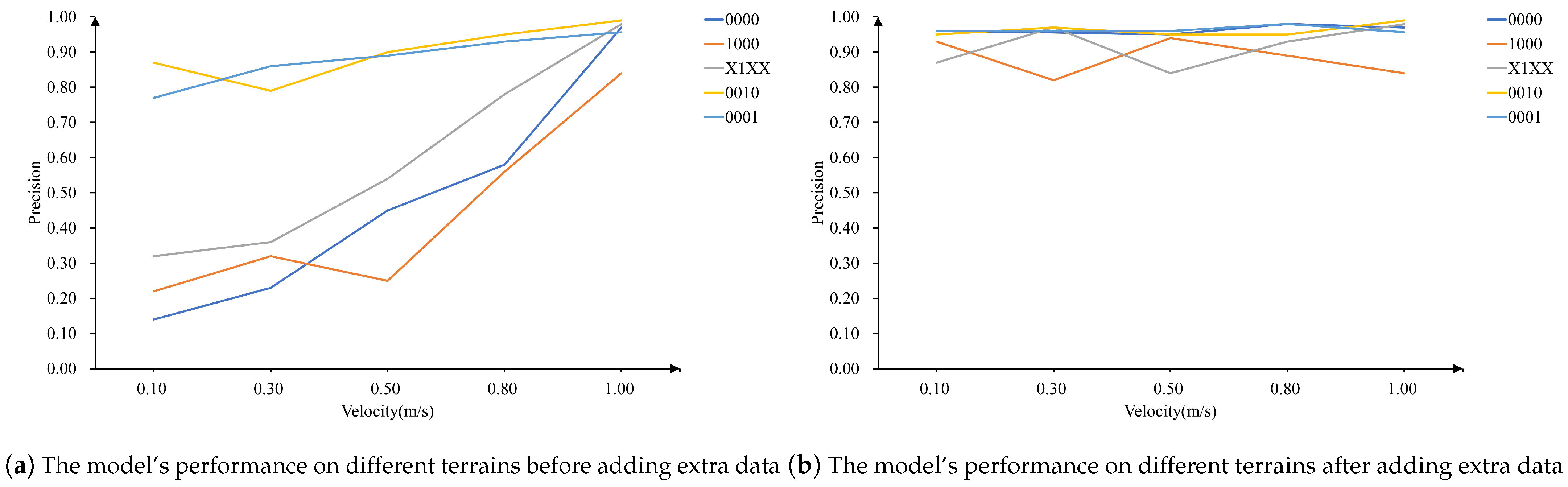
In addition to the experiments on motion patterns, experiments on the impact of robot speed on the model were also conducted. Specifically, a model trained at a speed of v = 1 m/s was first evaluated to observe accuracy variations at different speeds. Then, data from various speeds was added to the training set for retraining, and changes in model performance across different velocities were analyzed.

4. Result and Analysis

4.1. Precision Analysis

Table 2. The classification accuracy table with different backbones.

Algorithms	0000	1000	X1XX	0010	0001	Average
EfficientNet	93.64%	60.70%	95.40%	97.90%	84.98%	86.52%
MobileNet	96.19%	76.12%	70.71%	100%	96.44%	87.89%
ResNet-18	95.34%	84.58%	92.89%	94.59%	95.65%	92.61%
ResNet-34	92.80%	82.59%	97.91%	96.70%	96.44%	93.29%
ResNet-50	97.46%	93.53%	85.77%	95.20%	96.05%	93.60%
Inception-ResNet V2	96.19%	94.03%	84.52%	95.80%	96.05%	93.32%
Transformer	85.59%	70.65%	89.54%	89.79%	87.75%	84.66%

presents the experimental results of replacing the backbone model in the heatmap branch. Based on the comparative experiments in Table 2, it is evident that the performance of the ResNet series networks (ResNet-18, ResNet-32, ResNet-50) in this study is quite similar. The classification accuracy did not increase with the deepening of the model layers. However, from the experimental results of the MobileNet and EfficientNet models, it can be observed that the lightweight design does indeed have a noticeable impact on model accuracy.

Additionally, based on the results of Transformer and Proprioception Net, transforming the multi-sensor fusion task into a pure time-series problem is not as effective as processing the time-series signals into two-dimensional image signals. The primary reason is that 2D convolutions can simultaneously learn features along the temporal axis and across sensor channels. Furthermore, the data used in this study consist of raw data with minimal secondary processing, which makes Transformers more susceptible to noise interference.

Table 3. The classification accuracy table for different multi-sensor fusion models.

Algorithms	0000	1000	X1XX	0010	0001	Average
Proprioception Net	10.17%	79.10%	97.07%	94.29%	84.58%	73.04%
MLP	80.93%	73.13%	84.94%	88.89%	88.14%	83.21%
LMSCNN	94.92%	80.10%	74.90%	96.70%	98.02%	88.93%
MmA	91.10%	83.08%	81.17%	93.99%	92.89%	88.45%
Proposed	97.46%	84.08%	97.91%	100%	95.65%	95.02%

provides accuracy comparison between the different multi-sensor fusion model. In the Proprioception Net, the architecture employs a 1D convolutional neural network, but it fails to capture relationships between sensors and has shallow network depth, resulting in the lowest average accuracy on the dataset. The MLP model requires handcrafted feature engineering and exhibit limited nonlinear modeling capacity, resulting in the lowest accuracy on Dataset “1000”, which has the highest nonlinearity. In the LMSCNN, the MBConv block is used and integrates a classifier for fault classification. Regarding the MmA model, this study also used ResNet as the feature extraction branch and concatenated the vectors of various sensor waveforms into one vector as shared representation. Multiple classifiers were then added after the shared representation to obtain a separate classifier for each terrain type, which also yielded some gains but was not significantly different from the backbone.

4.2. Ablation Study

In the ablation experiments, the time-dependent feature branch and the heatmap feature branch were successively removed to evaluate the effects of each branch. As shown in

Table 4. The classification accuracy table for the ablation study.

	0000	1000	X1XX	0010	0001	Average
Without time-dependent feature branch	95.34%	84.58%	92.89%	94.59%	95.65%	92.61%
Without heatmap feature branch	93.22%	75.62%	85.36%	88.59%	77.87%	84.13%

, when the heatmap feature branch is removed, the model can only extract features along the temporal axis and fails to effectively learn the relationship between sensor data, resulting in suboptimal performance. Correspondingly, removing time-dependent features results in the loss of temporal characteristics in the temporal data.

As shown in Figure 11, this study tested the model accuracy when individual sensor signals were systematically removed. In the experiments, multiple sensor signal inputs were sequentially masked (set to zero) to observe the model’s performance. We can observe that the vibration data play an important role in the labels “1000”, “X1XX”, and “0001”, while the foot-end velocity has the greatest impact on the label “0000”. Additionally, the body’s angular velocity has negligible effects across all labels, implying that the angular velocity signal could be removed to reduce computational costs.

4.3. Effect of Motion Patterns

To demonstrate the influence of motion patterns on model accuracy, the proposed model was tested on terrain data with different motion patterns. It can be seen that there is a significant drop in model accuracy, and the model becomes less reliable, which undoubtedly confirms the hypothesis initially proposed in this study. However, when the model incorporates information about the relevant motion patterns into the training data, the impact of the motion patterns is mitigated. As shown in Figure 12, the model accuracy improves.

Similarly, as illustrated in Figure 13, the model trained at a velocity of 1 m/s demonstrates performance variations when tested at other velocities. The classification accuracy of labels “0000”, “X1XX”, and “1000” shows significant sensitivity to variations in movement velocity. However, this impact is mitigated after supplementary training with multi-velocity data.

5. Conclusions

Ground information perception for robots is crucial for enhancing robot performance and traversal capabilities. This study addresses the shortcomings of existing technologies and thoroughly analyzes the characteristics of previous multi-sensor fusion algorithms. We propose the use of a time-dependent feature branch to capture features from the temporal axis and employ a heatmap feature branch for extracting relational features between sensor signals. From the results of the ablation experiments, it is evident that each component contributes significantly to the model’s accuracy.

Furthermore, according to the comparative experimental results, the proposed model exhibits superior accuracy and robustness compared to existing multi-sensor fusion algorithms, achieving a test accuracy of 95.02%. The training data required by this method are easy to obtain and only require an IMU sensor and a joint encoder sensor installed on the robot.

In the fusion experiments, the proposed model demonstrates reliable classification accuracy even when some data are missing. Additionally, the experimental results regarding the impact of motion patterns on model accuracy indicate that changes in motion patterns significantly affect model accuracy and reliability. This study also proposes a method to eliminate the impact of motion patterns by adding training samples containing various motion patterns, effectively mitigating the influence of inherent motion patterns. Although this method has been experimentally verified to be reliable and effective, there are still limitations that need to be pointed out:

(1)

The experiments only conducted terrain classification experiments on a limited set of terrains. Due to experimental conditions and time constraints, additional complex terrains with coupled multi-labels have not been tested.

(2)

The slippage terrain used in this study is flowing terrain. In fact, the slippage characteristics caused by slippery tiles (e.g., wet floors) may differ significantly from those caused by flowing terrains (e.g., sand or snow). Therefore, we cannot predict the model’s performance in such slippage terrains.

(3)

Regarding the motion-pattern-independent experiments, in order to test the performance of the motion-pattern-independent model, additional training data containing different motion information were used. This implicitly provided the model with information about motion patterns. However, the model can still be affected by new motion patterns that are not included in the training data.

In future work, we will conduct experiments on more complex, unstructured terrains where various hazardous road conditions are coupled. Additionally, we will attempt to integrate terrain physical characteristic labels into the control framework. Specifically, we aim to incorporate these labels into a dynamics-based MPC control framework, allowing real-time adjustments of control parameters and expected ground reaction forces based on terrain perception results. This will enhance the quadruped robot’s traversability.