Fault Diagnosis Method for Sub-Module Open-Circuit Faults in Photovoltaic DC Collection Systems Based on CNN-LSTM

Abstract

To diagnose open-circuit faults (OCFs) in sub-module switching devices within input-independent output-series (IIOS) photovoltaic DC collection systems, this paper presents a hybrid diagnostic method combining convolutional neural networks (CNNs) and long short-term memory networks (LSTMs). The method utilizes a sliding window technique to segment sub-module capacitor voltage signals into time-series samples. Initially, CNN automatically extracts local features from the samples, followed by LSTM for capturing temporal dependencies and extracting global time series features, enabling effective fault detection under complex conditions. This approach eliminates the need for manual feature extraction and complex system modeling. By leveraging the model’s learning capabilities, it mitigates the impact of solar irradiance fluctuations on diagnostic accuracy. After training, the model performs real-time fault diagnosis with high precision using voltage data, offering fast, efficient, and reliable performance. The effectiveness of the method was validated through both simulation and experimental results.

1. Introduction

With the continuous growth of photovoltaic (PV) installed capacity and the increasing share of power generation, along with advancements in power electronics and flexible DC transmission technology, DC aggregation is expected to replace traditional AC grid connection methods, becoming a key approach for PV power generation integration [1]. Due to their low power density, PV arrays often require a boosting and aggregation system to achieve reliable grid connection [2,3]. Currently, DC pooling technologies are mainly based on two cascade topologies: input-independent output-series (IIOS) and input-parallel output-series (IPOS) [4,5]. The IIOS-type topology indicates that each PV array is connected to the grid through independent inputs, and then the outputs are connected in a series after boosting, while the IPOS-type topology has inputs connected in parallel and outputs connected in series. Pure IPOS does not allow for all the PV panels to operate at the maximum power point, and it is necessary to add a first-stage converter for all the PV arrays to realize their own independent maximum power point tracking (MPPT) prior to pooling. The IIOS topology offers significant advantages over IPOS, including independent MPPT on the input side and a high boost ratio on the output side. This architecture is particularly suited to photovoltaic DC collection systems in medium-voltage environments, as it reduces system costs, eliminates the broadband oscillation issue of multiple inverter cascades, and offers higher efficiency and stability [5,6,7]. Moreover, to mitigate fluctuations in PV output and improve a voltage imbalance due to a power mismatch, IIOS-type photovoltaic DC systems with additional balancing modules have been proposed [8,9]. These systems can transfer mismatched power between PV modules, equalizing output voltage and enhancing system efficiency. However, the addition of balancing modules increases the number of switching devices, and studies show that the probability of damage to power devices in power electronic converters can be as high as 21% [10]. Furthermore, with the growing number of sub-modules (SMs), the likelihood of fault occurrence increases, making the fault diagnosis of SM switching devices critical for enhancing system reliability.

Switching tube faults in SM primarily include short-circuit faults (SCFs) and open-circuit faults (OCFs). Typically, SCFs evolve into OCFs under the isolation effect of hardware protection devices [11]. As a result, most research focuses on OCF diagnosis methods. There are three primary approaches to diagnosing OCFs in converter switching devices: hardware-based, model-based, and machine learning-based methods.

Hardware-based diagnostic methods rely on real-time monitoring using sensors and additional circuitry to detect faults quickly. Although these methods offer fast response times and high reliability, they are not suitable for large-scale PV systems due to the additional sensors and circuits required, which increase costs and system complexity. Additionally, these methods struggle with environmental adaptability and are prone to interference from other faults and external disturbances [12,13]. Model-based fault diagnosis methods detect faults by constructing a mathematical model of the system and identifying deviations between observed and predicted values. For example, reference [14] used a state observer to detect faults by solving the deviation between measured and calculated values, while reference [15] proposed an incremental prediction model that adjusts parameters to diagnose faults. However, this approach requires the careful setting of fault thresholds, as small thresholds may lead to false positives and large thresholds may miss early-stage faults. Furthermore, model-based methods are sensitive to changes in system parameters, and the accuracy of the model directly influences diagnostic performance. This can be especially problematic when environmental changes or significant parameter fluctuations occur.

Traditional machine learning (ML) methods generally involve two stages: manual feature extraction and fault classification. For instance, reference [16] employed principal component analysis to extract fast Fourier transform features of the output voltage, and used a multiclass correlation vector machine for fault classification. Similarly, reference [17] extracted fault features by collecting the bridge arm current signal of modular multilevel converters (MMC) and combining LSTM with support vector machines (SVM) for classification. However, these traditional ML methods heavily depend on expert knowledge for feature design and adjustment, making it difficult to fully exploit the deep information contained in the data. In contrast, deep learning offers better adaptability for diagnosing complex fault patterns through automatic feature extraction. Aung et al. proposed a fault detection system based on embedded machine learning and performed real-time condition monitoring through CNN [18].Reference [19] demonstrated the use of adaptive 1D-CNN to collect raw voltage and current data from MMCs for fault detection, achieving excellent accuracy and reliability, but requiring large datasets and being susceptible to overfitting. Reference [20] applied stacked sparse autoencoders (SSAEs) for unsupervised learning on voltage samples, followed by a Softmax classifier for fault diagnosis. However, SSAE suffers from challenges such as difficult parameter tuning and limited local feature capture.

Existing methods have mainly been applied to OCF diagnosis in MMC sub-modules. However, diagnosing switching-tube OCFs in IIOS-type DC pooling systems is more challenging due to the impact of PV fluctuations and balancing modules. To address this, this paper proposes a CNN-LSTM-based fault diagnosis method. The method utilizes CNN for automatic deep feature extraction, reducing manual effort, followed by LSTM to capture temporal features and improve fault diagnosis accuracy. This approach enables the early and accurate identification of fault types, even under complex conditions.

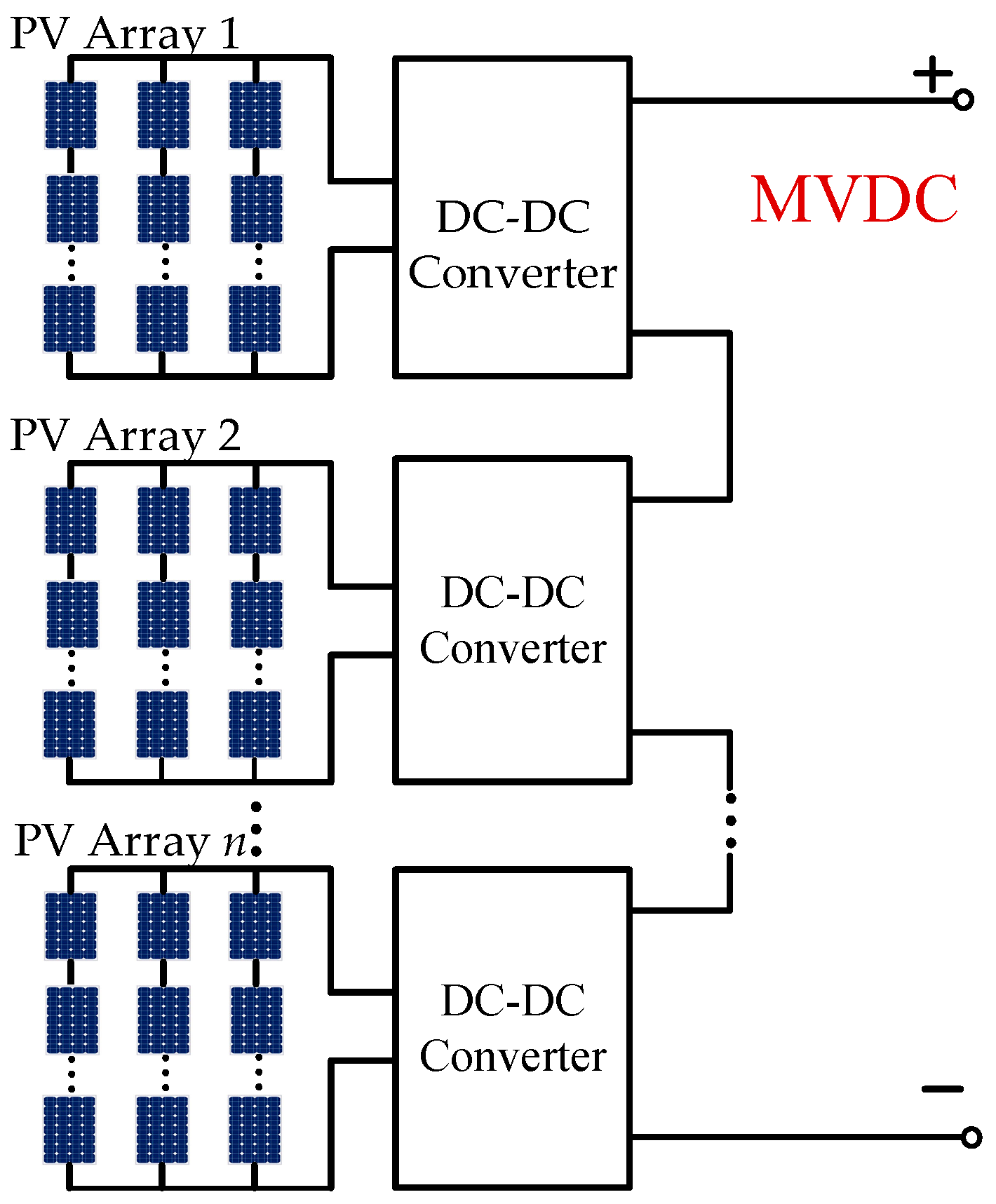
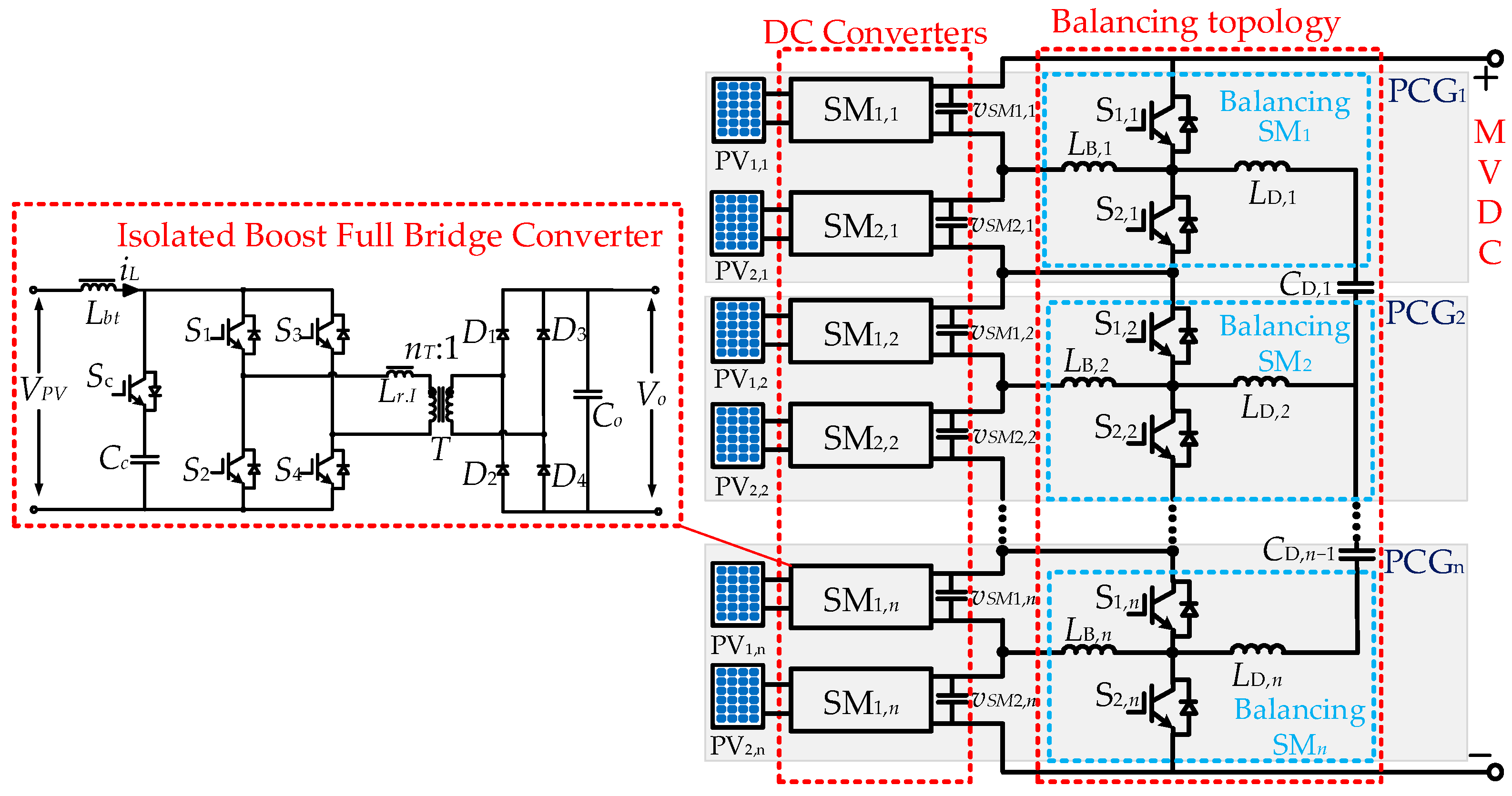
2. Principle of Operation and Fault Characteristics

Photovoltaic DC collection systems are usually applied in medium-voltage-distributed PV power generation scenarios. According to the insulation requirements, the output voltage of PV arrays is usually designed to be no more than 1 kV, while the medium-voltage direct current (MVDC) scenarios are usually 10 kV or 35 kV, so for the photovoltaic DC collection system, a high boost ratio photovoltaic DC boost converter is the key to the system. The IIOS-type photovoltaic DC collection system shown in Figure 1 is a suitable choice, which realizes independent maximum power point tracking (MPPT) by connecting PV cells at each input port. The output series structure achieves a high boost ratio, which meets the needs of a photovoltaic DC collection system in medium-voltage environments.

In the PV DC collection system, the interface converter for PV sub-modules is selected as an isolated boost full-bridge converter (IBFBC) [21]. The topology of the IBFBC is shown in Figure 2. In this topology, L_bt is the Boost inductor, power switches S₁–S₄ form the primary-side full bridge, and diodes D₁–D₄ constitute the uncontrolled secondary-side full bridge. The high-frequency transformer T has a turns ratio of n:1, while Co is the output filter capacitor.

The main problem of the IIOS structure is that since the output voltage of each sub-module is proportional to its input power, a power mismatch occurs under uneven illumination, which leads to the unbalanced output voltage of each PV sub-module. When the power mismatch is severe, the output voltage of each sub-module will also be severely unbalanced, and some PV sub-modules are unable to maintain the MPPT because the output-side partial voltage is too low; other modules may be damaged due to the output-side partial voltage being too high, which results in the device being subjected to too high a voltage stress. Therefore, it is necessary to attach a power balancing sub-module to the PV output port [22], of which the topology is shown in Figure 2. This balancing sub-module effectively realizes the MPPT and voltage equalization decoupling control of the convergence system and improves the operational stability of the collection system.

The topology of the IIOS-type photovoltaic DC collection system with balancing modules in this paper is shown in Figure 2, which consists of n independent input SMs and n/2 dual-path balancing modules. Among the SMs, an isolated boost full-bridge converter (IBFBC) is selected to realize independent MPPT control. The balancing module consists of a half-bridge and two inductors, and two adjacent balancing modules are connected to each other by a capacitor. It realizes the direct transfer of mismatched power between the SMs, and then effectively realizes the output side voltage balancing.

2.1. Sub-Module Operation Principle

The converter IBFBC topology used for the SM in the front stage of the system is shown in Figure 2, where a boost inductor is added to the input side of the full-bridge converter, which can be equated to an isolated Boost circuit.

In this paper, IBFBC is used to realize independent MPPT control of each SM in steady-state operation, in which S₁, S₃, and S₄ form a controllable full-bridge circuit with power switching tubes S₁, S₂, S₃, and S₄; T is a high-frequency AC transformer; Lr is its leakage inductance; D₁, D₂, D₃, and D₄ are uncontrolled full-bridge rectifier diodes; C_o is the output filtering capacitance; and IBFBC has the advantages of galvanic isolation and high step-up ratio, and it is very suitable for photovoltaic DC collection systems that require galvanic isolation and have a high-voltage DC bus during the system. In this paper, the IBFBC was used to realize the independent MPPT control of each SM, and in the steady-state operation, the duty cycle of switching tubes met 0.5 < D < 1.0, in which the S₁ and S₄ conduction signals were the same, and the conduction signals of S₂ and S₃ had a 180° phase difference with S₁ and S₄, and S_c was delayed to conduction only in the diagonal tube conduction of the bridge arm. Reference [23] describes the working principle of the IBFBC in more detail, which will not be expanded in this paper.

The topology of the balancing module is shown in Figure 2 with two power transfer paths, and each balancing module connects two PV sub-modules. For ease of analysis, two PV sub-modules and one balancing module are defined as a power converter group (PCG). Within this structure, inductor L_B,n is employed to facilitate power balancing within PCG, while inductor L_D,n is responsible for balancing power between PCGs. The operating principles of the two balancing paths in the balancing module are described in detail below.

When only internal balancing within PCG is considered, the inductor L_D and capacitor C_D can be disregarded, and the system can be represented as a Buck–Boost converter. The switching devices in the upper and lower bridge arms of the balancing unit operate in a complementary manner, with a fixed duty cycle of 50%. This configuration allows for voltage balancing at the outputs of adjacent SMs through the charging and discharging of L_B.

When the focus shifts to balancing between PCGs, inductor L_B,n can be neglected, and the system can be simplified to a half-bridge inverter. These two half-bridge inverters are interconnected by the inductor, L_D, and several capacitors, C_D. Each half-bridge inverter converts the DC output from the SM into a phase-controlled AC source, enabling power transfer between SMs by adjusting the phase shift between switches S_1,1 and S_1,n, thus achieving voltage balancing across the groups.

2.2. Sub-Module Fault Characteristics

The OCFs of the SM were first analyzed. When the SM has an IGBT OCF, using an OCF in S₁ as an example, the four fault circuits formed by the IBFBC are shown in Figure 3.

It can be seen that when the four switching tubes are conducting, an OCF in S₁ will form fault loop 1, at which time S₃ and S₄ are still conducting, consistent with normal operation, and L_bt is in the charging stage. When S₁ and S₄ are just conducting and an OCF occurs in S₁, as shown in fault loop 2, then S_c is not yet conducting and current flows to C_c, which begins to charge while i_Lbt decreases. When S₁ and S₄ conduct for a period of time, an OCF occurs in S₁ which will form fault circuit 3, at which time S_c has conducted, C_c continues to charge, and the primary side of the transformer forms a continuation circuit through S₁ and S₄. Subsequently, when S₂ and S₃ conduct and an OCF occurs in S₁, it corresponds to fault loop 4, which temporarily maintains the normal state, and Lbt transmits power to the secondary side of the transformer. For the other IGBTs in the IBFBC that have OCFs, the fault analysis is similar to that of S₁, and after the occurrence of an OCF, it is manifested as a drop in C_o voltage and a decrease in transformer leakage inductance current, at which time, the faulty sub-module capacitance voltage decreases, and the dividing voltages of the capacitors of the rest of the SMs will increase, but the SM capacitance voltages tend to be equalized under the effect of the balancing module.

When analyzing OCFs in the IGBT within the balancing module, if only the internal balancing of the converter group is considered, it is assumed that the output power of SM_1,n exceeds that of SM_2,n, and likewise, the output power of SM_1,n+1 surpasses that of SM_2,n+1. In this scenario, capacitors C_1,n, C_2,n, C_1,n+1 and C_2,n+1 represent the output-side capacitors of SM_1,n, SM_2,n, SM_1,n+1 and SM_2,n+1, respectively. Taking the case of an open circuit in S_1,n as an example, the balancing circuit may form two distinct fault circuits after the failure, as depicted in Figure 4a,b. When S_1,n and S_1,n+1 are conducting and an OCF occurs in S_1,n, the switches S_2,n and S_2,n+1 remain off. Consequently, L_B,n+1 enters a charging state, while inductor L_B,n cannot charge. Conversely, when both S_1,n and S_1,n+1 are off, and S_2,n and S_2,n+1 are conducting, L_B,n+1 enters a discharging state. However, due to the OCF in S_1,n, power cannot flow from SM_1,n to SM_2,n, causing an imbalance in the capacitor voltage of the SM, and disrupting the voltage balancing between SM_1,n and SM_2,n.

When inter-group balancing is considered, the fault modes of IGBT OCFs are analyzed by referencing PCG_n and PCG_n+1, under the assumption that the sum of the output powers of SM_1,n and SM_2,n exceeds that of SM_1,n+1 and SM_2,n+1. Let V_LD,n and V_LD,n+1 represent the voltage drops across inductors L_D,n and L_D,n+1, respectively, while i_CD,n denotes the current flowing through capacitor C_D,n. Taking the OCF in S_1,n as an example, the four potential fault circuits that could form in the balancing circuit are shown in Figure 4c–f.

When S_1,n and S_1,n+1 conduct and an OCF occurs in S_1,n, switches S_2,n and S_2,n+1 remain off, preventing the charging of capacitor C_D,n. When S_2,n and S_1,n+1 conduct while S_1,n and S_2,n+1 are off, a closed loop is formed: S_2,n-L_D,n-C_D,n-L_D,n+1-S_1,n+1. In this configuration, V_LD,n is negative, and V_LD,n+1 is positive. Consequently, the current i_CD,n rapidly decreases from positive to negative, preparing the capacitor C_D,n for discharge in the next phase. When S_2,n and S_2,n+1 are on, and S_1,n and S_1,n+1 are off, the open circuit in S_1,n causes capacitors C_1,n+1 and C_2,n+1 to charge C_D,n. However, since the sum of the output power of SM_1,n and SM_2,n is greater than that of SM_1,n+1 and SM_2,n+1, power cannot flow from PCG_n+1 to PCG_n.

Finally, when S_1,n and S_2,n+1 conduct, and S_2,n and S_1,n+1 are off, a closed loop is formed through C_o1,n-C_o2,n-C_o1,n+1-C_o2,n+1-S_1,n-L_D,n-C_D,n-L_D,n+1-S_2,n+1. At this point, V_LD,n is positive, and V_LD,n+1 is negative. The current i_CD,n rapidly rises from negative to positive, preparing capacitor C_D,n for charging in the subsequent stage. It is evident that when an OCF occurs in S_1,n, the system is unable to achieve inter-group balancing, leading to an imbalance in the capacitor voltage of the SM.

In the case of an OCF in the switching devices within the system SMs, the capacitor voltage of the faulty SM decreases, which results in a reduction in the system’s output power. An open-circuit failure in the balancing module causes the capacitor voltage of the corresponding SM to fluctuate under the influence of the PV collection system, preventing both intra-group and inter-group balancing. This condition may further damage the system components, thereby compromising the system’s reliability. Therefore, diagnosing open-circuit failures in switching devices is critical for maintaining the stability and reliability of photovoltaic DC collection systems.

After clarifying the working principle and fault characteristics of the type IIOS PV DC pooling system, the next step will be to introduce how to utilize the CNN-LSTM model to achieve efficient and accurate fault diagnosis.

3. Fault Diagnosis Method Based on CNN-LSTM

3.1. Principles of CNN-LSTM Model

There are many SMs in the photovoltaic DC collection system and the operating conditions are complex, which makes it difficult to extract fault features. In this paper, CNN was used to automatically extract fault features. CNN is a deep learning model specialized in processing data with network organization, which automatically extracts and classifies features in the data through its convolutional kernel. The CNN model consists of an input layer, a convolution layer, a pooling layer, and a fully connected layer [24]. Among them, the convolution layer uses the convolution kernel to perform convolution operations on the local area of the input feature map, and generates multiple sets of output feature maps through a nonlinear activation function. Relying on the weight sharing mechanism, the convolution layer not only simplifies the training process of the model, but also significantly reduces the number of parameters. The mathematical expression of the convolution layer is as follows:

$${x_j}^l=f({\displaystyle \sum _{i=1}^M{X_j}^{l-1}\times {k_{ij}}^l+{b_j}^i})$$

(1)

where x_j^lrepresents the jth feature map in the lth layer; f is the activation function; M is the number of input feature maps; k_ij^l is a trainable convolution kernel; and b_jⁱ represents the bias term.

The operation of the pooling layer is completed by the pooling kernel, which is processed by traversing and scanning the feature matrix generated by the convolutional layer. Its mathematical formula is

$${y_i}^{l+1}(j)=\max \left\{\underset{k\in D_j}{{\displaystyle {x_i}^l}}(k)\right\}$$

(2)

Among them,x_j^l(k) is the element of the jth feature matrix of the lth layer in the coverage area of the pooling core; y_i^l+1(k) is the element of the i-th feature matrix of the l + 1th layer after pooling; and D_j is the coverage range of the jth pooling core. Through sparse connection and a weight sharing mechanism, CNN can directly extract local features from raw data and realize automatic feature extraction.

LSTM is a special kind of recurrent neural network (RNN) for processing sequence data, which solves the problems of gradient vanishing and gradient explosion of traditional RNNs in processing long sequences by introducing memory units and gating mechanisms, and is able to capture long-term dependencies better [25]. Its model architecture is shown in Figure 5. The LSTM model dynamically adjusts the information flow by introducing forget gate, update gate and output gate, thereby effectively extracting the temporal features of time series data. Its main steps are as follows:

The forget gate combines the previous hidden state h_t−1 and the current input x_t, and determines the amount of previous information that needs to be discarded through the σ activation function. The formula is

$$f_{\mathrm{t}}=\sigma [W_f(h_{t-1},x_t)+b_f]$$

(3)

The update gate determines the information that can be added to the current memory state through the σ activation function, and generates a new candidate memory vector ${\tilde{C}}_t$ using the tanh activation function, which is formulated as follows:

$$\left\{\begin{array}{l}{i}_t=\sigma [W_i(h_{t-1},x_t)+b_i]\\ {\tilde{C}}_t=\tanh [W_c(h_{t-1},x_t)+b_c]\\ C_t=ft{C}_{t-1}+i_t\times {\tilde{C}}_t\end{array}\right.$$

(4)

The output gate generates the final network output o_t based on part of the current memory state.

$$\left\{\begin{array}{l}{o}_t=\sigma [W_o(h_{t-1},x_t)+b_o]\\ h_t=o_t\tanh (c_t)\end{array}\right.$$

(5)

Among them, W and b are the weight matrix and bias vector, respectively.

LSTM has deficiencies in local feature learning and is difficult to effectively extract fault features, while CNN cannot capture the temporal characteristics of SM faults. The CNN-LSTM model combines the advantages of CNN in feature extraction and the strengths of LSTM in time series data processing. By combining the convolution layer with the LSTM layer, the prediction model can extract significant features from the original data and capture the temporal features hidden in the historical trend. The CNN-LSTM fault diagnosis model constructed in this paper is shown in Figure 6. The model consists of an input layer, a convolution layer, a pooling layer, an LSTM layer, a fully connected layer, and an output layer. Among them, the pooling layer down-samples the output vector of the convolution layer, which is equivalent to secondary feature extraction. In order to optimize the performance of the model, a random dropout layer (Dropout) and a Flatten layer are added on this basis. The Dropout layer is used to solve the common overfitting problem in deep neural networks and improve the generalization performance of neural networks [26]. The Flatten layer is used to adjust the data format to the input format required by the LSTM layer. The fully connected layer is used to integrate and classify the extracted features.

3.2. Fault Diagnosis Model Based on CNN-LSTM

This paper selects the SM capacitor voltage as the raw data for open-circuit fault diagnosis, and combines the model theory in the previous section to propose a CNN-LSTM-based open-circuit fault diagnosis method. The model construction process is shown in Figure 7, which mainly includes data acquisition, data preprocessing, model training, and real-time diagnosis, which will be discussed below.

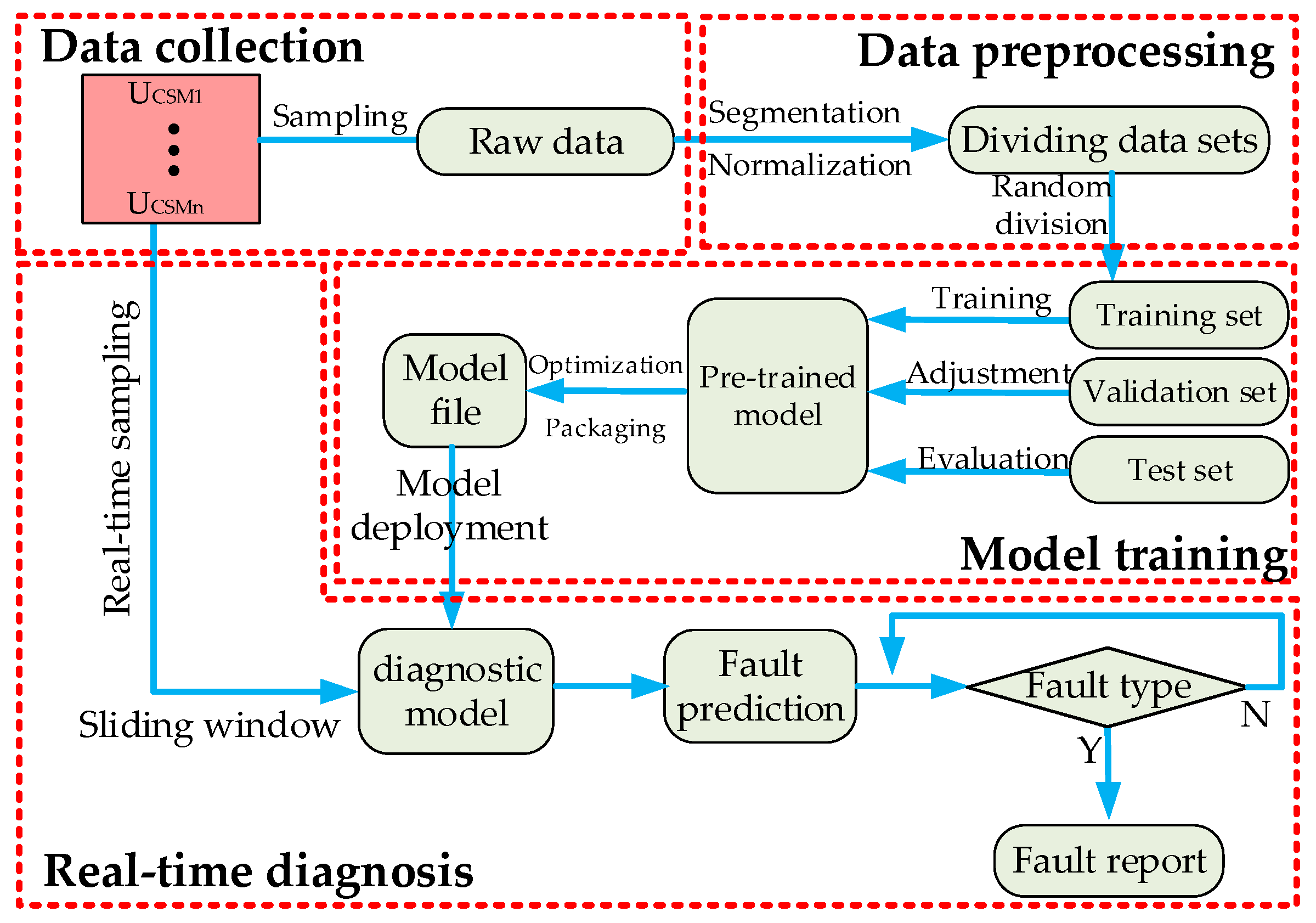
3.2.1. Data Collection

In the analysis of the system’s transition from normal operation to a fault condition, multi-channel signals corresponding to the SM capacitor voltage are sampled. The resulting signal dataset, denoted as X, is assumed to be an m × n matrix, where n represents the total number of sampling instances and mmm corresponds to the number of signal channels. The individual components of the dataset, X_j (j = 1, 2, …, n), are defined as follows:

$$X_j={[X_{1j},X_{2j},\cdot \cdot \cdot ,X_{(m-1)j},X_{mj}]}^T$$

(6)

Upon collecting the SM capacitor voltage data, a fault label is assigned according to the fault type outlined in

Table 1. Open-circuit fault label.

Label	Fault Type
F0	Normal
F1~F10	PV sub-modules (SM1-S1~SM10-S1)
F11~F20	Balancing sub-modules (S1,1,S2,1~S1,5,S2,5)

, where F₀ represents the label for the normal state. By varying the light intensity and fault occurrence time, voltage changes of the SMs capacitor are recorded as the system transitions from normal to fault states, under different operating conditions. This process facilitates the creation of the dataset required for model training.

3.2.2. Data Preprocessing

The raw data samples obtained are then subjected to preprocessing, the preprocessing of the raw SM capacitance and voltage data involves the following steps.

This paper uses the sliding window method to segment the collected data to obtain data samples for fault diagnosis, while realizing the dynamic update of sensor collected data. The processing flow of the sliding window on the sampled data is shown in Figure 8.

After acquiring the SM capacitor voltage sampling data, the original sequence is divided into windows of length, L. Each interception generates a data segment of length, L, and slides backward from the starting point of the original sequence with a step size of ΔL to generate new data segments in sequence. The sampled voltage sequence is processed by the sliding window, and the intercepted segments eventually constitute a data sample set. The selection of the sliding window size should ensure that the intercepted segments can fully contain the feature information. Increasing the sliding window length can include more feature information in the sample to improve the diagnostic accuracy, but it will also increase the demand for computing resources and diagnostic time. The selection of the sliding step size affects the accuracy of the fault diagnosis time point. Reducing the step size can improve the diagnostic accuracy, but it will also increase the complexity of data processing and the hardware memory requirements.

In order to reduce the impact of the local amplitude change of the capacitor voltage when a fault occurs, the numerical scale difference id reduced and the model training efficiency improved. This paper normalizes the sample data of each channel. Through the normalization method based on the maximum and minimum values of the sample in Formula (7), the data are mapped to the [0, 1] interval, thereby concentrating the numerical distribution of the input data, improving the calculation stability and enhancing the generalization ability of the model.

$$V^{\prime }={\displaystyle \frac{V-V_{\min }}{V_{\max }-V_{\min }}}$$

(7)

To enhance the data diversity and mitigate overfitting, this study applies data augmentation techniques. Specifically, small Gaussian noise is added to the original dataset for each fault type, thereby augmenting the data. This process not only increases the robustness of the model, but also improves its diagnostic accuracy. Additionally, fault samples are further simulated by introducing time offsets. The dataset is then randomly split into training, validation, and test sets, with proportions of 70%, 15%, and 15%, respectively. The training set is used to optimize model parameters and learn the underlying patterns in the data through iterative updates; the validation set is utilized to adjust hyperparameters and assess the model’s performance on unseen data to prevent overfitting; the test set is employed to evaluate the model’s generalization capability and performance in real-world scenarios. This division method enhances both model training and hyperparameter tuning efficiency, while ensuring reliable performance evaluation, ultimately strengthening the model’s ability to generalize across diverse data distributions.

3.2.3. Model Training

In this study, we determined the optimal hyperparameters of the CNN-LSTM model, including convolutional kernel size, number of nodes in the LSTM hidden layer, Dropout rate, and learning rate, through grid search and cross-validation to obtain the best diagnostic accuracy and generalization performance. The fault diagnosis model proposed in this paper begins with a 64 × 10 image input layer for feature extraction. The core architecture includes two convolutional layers: the first layer uses a 3 × 33 filter with 8 channels, and the second layer uses a 3 × 33 filter with 16 channels. Each convolutional layer is followed by batch normalization and ReLU activation functions to enhance training stability and improve feature representation. A 2 × 2 pooling layer is then applied to down-sample the data, reducing its dimensionality and increasing computational efficiency. After the convolutional operations, the feature map is flattened and passed to an LSTM layer containing 64 neurons, which effectively captures temporal dependencies and time series features in the data. The model performs accurate fault classification through a fully connected layer followed by a Softmax layer.

Training employs the Adam optimizer with a maximum of 30 iterations, an initial learning rate of 0.001, and a segmented learning rate schedule that halves the learning rate every 10 iterations. The batch size is set to 64 to balance training efficiency and memory usage. To prevent overfitting, a Dropout layer with a rate of 0.4 is placed before the fully connected layer. Additionally, the dataset is randomly shuffled during each training epoch to further enhance the model’s generalization ability.

During training, the validation set is used to evaluate the model’s performance every 10 iterations, allowing for the real-time monitoring of convergence and performance fluctuations. The training and validation loss and accuracy curves are plotted during each epoch to offer a clear visual basis for model optimization and parameter adjustments. After training, the model is saved as an interface file and deployed in a real-time fault diagnosis system. Real-time voltage signals are continuously monitored, and fault types are predicted based on the highest probability calculated by the Softmax layer, thus enabling online fault diagnosis.

The fault diagnosis model processes real-time sampled capacitor voltage signals from the sub-modules, extracting continuous data segments. These segments undergo filtering and normalization to ensure signal quality and model stability. The preprocessed data are then fed into the trained CNN-LSTM model, which calculates the probability distribution of each fault type through the Softmax layer. The fault type is identified by selecting the class with the highest probability, ensuring efficient and accurate fault diagnosis.

4. Simulation and Experimental Verification

After elaborating the CNN-LSTM-based fault diagnosis method, the effectiveness and practical performance of the method are next verified in depth by simulation and experiment.

4.1. Simulation Verification

To validate the effectiveness of the proposed diagnostic method, a IIOS-type photovoltaic DC collection system model was constructed on the Matlab/Simulink platform. The system has a bus voltage of 10 kV, a rated power of 0.89 MW, and consists of five converter groups. Each PV sub-module has a rated output voltage of 1 kV, with additional parameters provided in

Table 2. Parameters of the simulation and experiment.

Parameter	Simulation	Experiment
DC bus voltage (Vbus)	10 kV	160 V
Nominal power (PG)	0.89 MW	600 W
Number of PV-SM (n)	10	4
Number of Balancing SM (n)	5	2
Switching frequency (fs)	1 kHz	1 kHz
PV sub-module parameter
Boost inductor (LBoost)	1 mH	500 uH
High-frequency transformer ratio	1:1	1:1
Input capacitance (Cin)	470 uF	940 uF
Output capacitance (Co)	1 mF	940 uF
Power switches selection	3300 V/400 A	BSC320N20NS3G
Balancing sub-module parameter
Balanced inductance in the group (LB)	6 mH	4 mH
Balanced inductance between groups (LD)	50 uH	100 uH
Capacitance between groups (CD)	250 uF	220 uF
Power switch selection	4500 V/400 A	IRFP250N

.

In the simulation, the corresponding gate signal is suppressed to simulate the open-circuit fault. According to the fault types in Table 1, 10 different fault time points and 10 groups of light intensity fluctuations are set for each fault type. The capacitor voltage signal is collected at a sampling frequency of 10 kHz, and a total of 2100 groups of data are obtained. The above preprocessing method is used to construct the dataset. After weighing, the sliding window length is set to 6.4 ms and the step size is set to 0.4 ms, and the total sample size is finally 5,216,400. The dataset is randomly divided into 70%, 15%, and 15%. The latest feature vector of each SM is extracted through the sliding window, and the trained model is loaded to predict its label to achieve fault diagnosis.

4.1.1. Diagnostic Accuracy Verification

The model was trained and tested using the collected sample set, and the accuracy of the diagnostic model reached 99.63%. The training progress curve is shown in Figure 9a. It can be seen that the model has a good learning effect, fast convergence speed and robustness. The verification accuracy is close to the training accuracy, indicating that the model performs consistently on different datasets, and the loss value has not increased significantly, indicating that the model is not overfitting. During the entire training process, the loss value of the model continued to decrease, indicating that the model is constantly learning and optimizing. Figure 9b is the confusion matrix of the diagnostic accuracy, which shows the percentage of classification results obtained after cross-validation of the final dataset. The classification of each fault type in the figure is mainly concentrated on the diagonal, which shows that the model has excellent fault diagnosis performance.

4.1.2. Model Comparison Analysis

In order to verify the superiority of the CNN-LSTM method, this paper combines it with other feature extraction algorithms and classification networks to conduct performance tests based on the same fault sample set to evaluate the feature extraction and recognition capabilities of this method. The training iteration accuracy and loss curves of each model are shown in Figure 10a.

The results show that CNN has the fastest convergence speed, the highest accuracy, and the model performance is relatively stable; LSTM has a slower convergence speed, and the convergence effect of the model is poor as the number of iterations increases; adding the stacked sparse autoencoder (SSAE) network to automatically extract fault features increases the accuracy to 89.91%, but SSAE has poor feature extraction effect on the fault information; in contrast, CNN-LSTM not only ensures the convergence speed and accuracy of the model, but also has smaller random fluctuations and loss values in the iteration process. Subsequently, a real-time diagnosis comparison analysis is performed through simulation, and the results are shown in Figure 10b. As can be seen from the figure, although the CNN model has a slightly faster diagnosis time, it has a misjudgment phenomenon due to the lack of global timing dependence; LSTM directly has an erroneous judgment, indicating that the model has not learned local fault features; adding SSAE-LSTM, the diagnosis time becomes longer, but misjudgment occurs in the normal state, indicating that the model has not extracted the fault features well; and the CNN-LSTM model in this paper has a slightly slower time than the CNN model, but its diagnosis accuracy is high, the classification effect is good, and there is no misjudgment.

The accuracy, F1 score, and diagnosis time of the model are shown in

Table 3. Performance comparison of different models.

Diagnostic Model	Accuracy (%)	F1 Score (%)	Diagnosis Time (ms)
CNN	95.11	92.35	1.8
CNN-LSTM	99.63	98.64	2.4
SSAE-LSTM	89.91	86.62	7.2
LSTM	78.74	70.87	3.6

. Among them, the F1 score is the harmonic mean of accuracy and recall, which can more comprehensively reflect the prediction performance of the model for fault classification. The results show that compared with the LSTM model, CNN model, and SSAE-LSTM methods, the CNN-LSTM model proposed in this paper has better diagnosis effect on SM open-circuit faults in photovoltaic DC collection systems under complex working conditions and has higher accuracy.

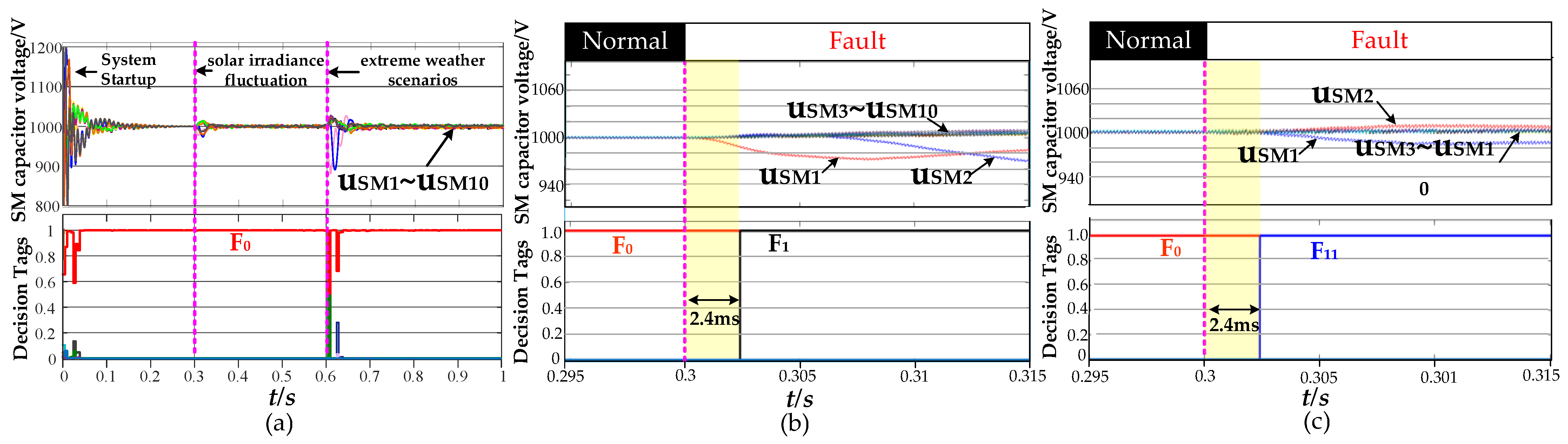
4.1.3. Real-Time Fault Diagnosis Verification

The trained model is deployed in Simulink for a real-time fault diagnosis simulation. The SM capacitor voltage data are collected in real time, processed by sliding windows, and then input into the deep learning toolbox to load and call the trained model interface file, and output the fault decision label. Figure 11a shows the graphs of SM capacitor voltages and model-determined labels during normal operation of the PV DC collection system after normal startup and addition of PV fluctuations. At 0.3 s and 0.6 s, the light intensity of SM₁ is reduced by 10% and 100%, respectively, to simulate the shading situation of the PV plant and the extreme weather scenarios. At this time, the SM capacitor voltage fluctuates and the voltage balance is achieved by the balancing module. The diagnostic decision label of the model always outputs F₀, which indicates that the diagnostic model does not make wrong decisions due to the variation of normal light intensity. The output of the model’s diagnostic fault type fluctuates during system startup and in extreme weather, but still the probability of F₀ is the highest and no misjudgment occurs. This shows that the model has excellent diagnostic results in different environments.

When an OCF occurs in S₁ of SM₁ at 0.3 s, as illustrated in Figure 11b, the voltage of the faulty SM capacitor drops following the fault. From the figure, it is evident that the fault type output indicates F₁ at 0.3024 s, confirming the detection and localization of the OCF in the S₁ of SM₁, with a diagnosis time of 2.4 ms.

Similarly, when an OCF occurs in the S_1,1 of the balancing SM₁ at 0.3 s, as shown in Figure 11c, the voltage of the SM fails to stabilize due to light fluctuations. The figure shows that the fault type output is F₁₁ at 0.3024 s, indicating the detection and localization of the OCF in the S_1,1 of SM₁, with a diagnosis time of 2.4 ms. These simulation results validate the effectiveness of the proposed fault diagnosis method.

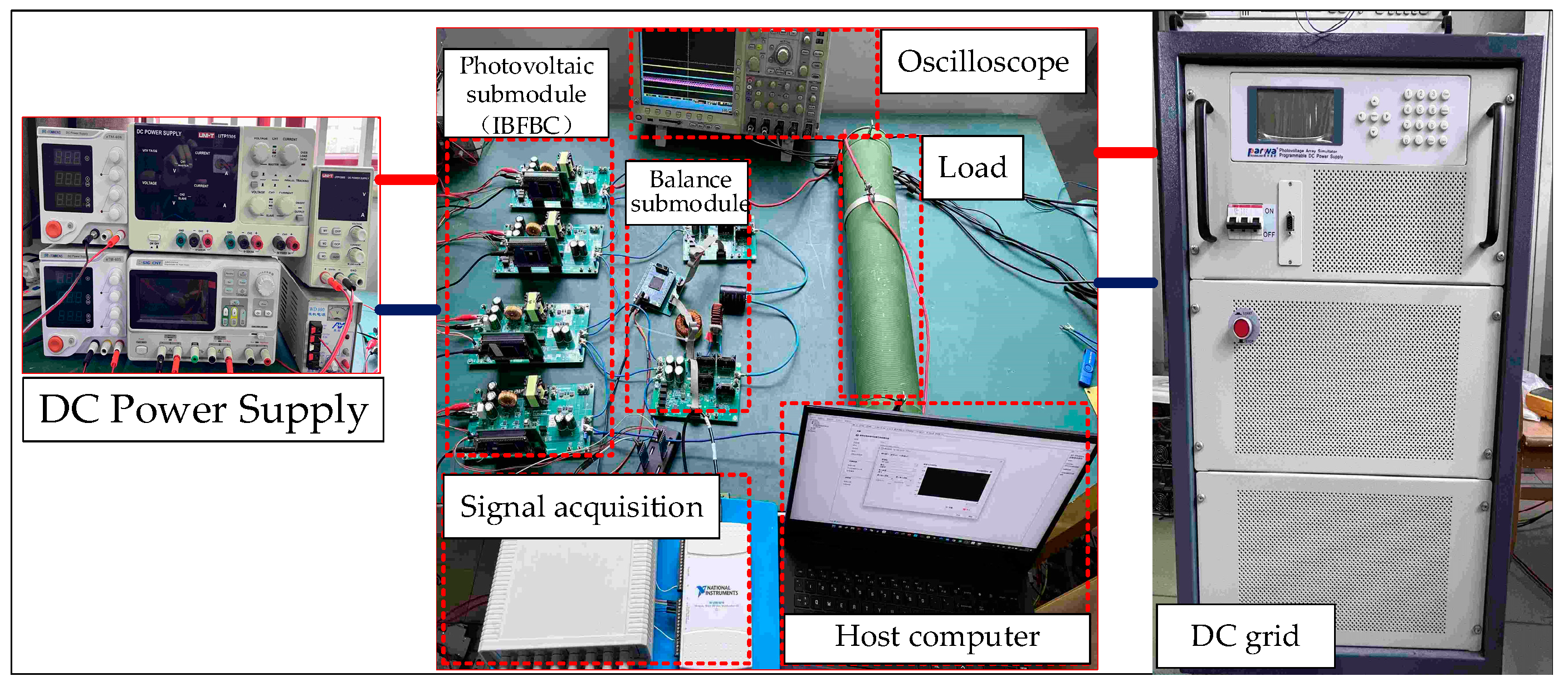
4.2. Experimental Verification

To further verify the proposed fault diagnosis technique, a small-scale experimental platform for a Photovoltaic DC collection system was constructed, comprising four IBFBCs and two balancing modules. The experimental parameters are listed in Table 2, and the experimental setup is illustrated in Figure 12. For simplicity, the IBFBCs use constant current controllers instead of MPPT controllers. The high-voltage side is connected to a load resistor, followed by a constant voltage source. The power is dissipated through the resistor, and the voltage on the high-voltage side is clamped by the constant voltage source to simulate a DC grid. Signal conditioning circuits and NI-DAQmx modules are used for data acquisition, while IGBT OCFs are simulated by blocking the corresponding gate drive signals.

A total of 36 experiments were conducted on the experimental platform, where the input power of each SM was adjusted by modifying the given current to simulate changes in illumination levels. Different fault types were introduced under varying light intensities, resulting in the collection of 144 sets of voltage data to construct the sample dataset. The sliding window length was set to 6.4 ms, with a step size of 0.4 ms, leading to a total sample size of 120,960. After collecting fault samples, the dataset was used to train the model and subsequently deployed on the host computer for real-time fault diagnosis experiments. These real-time fault diagnoses were carried out on a PC with a 2.20 GHz processor and 16 GB of RAM, using Matlab/Simulink 2024a. The Deep Learning Toolbox was employed to load the trained model and input real-time data for fault diagnosis.

• Fluctuation of light intensity under normal operation.

Figure 13a shows the experimental waveform when the current given value is reduced by 10% at time t₁, simulating a change in light intensity while the DC collection system operates normally. As shown, the SM output voltage fluctuates but is quickly stabilized by the balancing module. The decision output from the diagnostic model remains F₀, indicating no fault detection, and no misjudgment occurs.

• IBFBC-S₁ open-circuit fault

The diagnostic experiment waveform is shown in Figure 13b. It can be seen that when an open-circuit fault occurs in S₁ in SM₁ at time t₂, uSM1 decreases. After 7.2 ms, the diagnostic model diagnoses the specific fault location to achieve fault diagnosis and location.

• Balancing SM S_1,1 open-circuit fault

The waveform of the OCF diagnosis experiment of the balancing module S_1,1 is shown in Figure 13c. The driving signal of S_1,1 is cut off at time t₃ to simulate its OCF. It can be seen that under the simulated photovoltaic fluctuation, the OCF of the balancing module S_1,1 causes the capacitor voltage balancing failure. The diagnostic model detects and locates the specific fault location after 7.2 ms.

The diagnostic time in the experiment is longer than that in the simulation, mainly due to the limitation of hardware computing power. In addition, the sampling signal in the experiment needs to undergo additional signal conditioning, which increases the delay of signal processing and makes the noise interference in the experimental environment more significant. The experimental results show that the fault diagnosis method proposed in this paper can realize the rapid and accurate diagnosis of SM open-circuit faults in PV collection systems.

5. Discussion

The CNN-LSTM model-based sub-module open-circuit fault diagnosis method for photovoltaic DC convergence system proposed in this paper demonstrates excellent performance and practicality.

• The method automatically extracts local features through CNN and combines the capture of timing features by LSTM to realize efficient identification and localization of faults under complex working conditions. Simulation and experimental results confirm that the method has high diagnostic accuracy and robustness, and no obvious misdiagnosis occurs in complex environments such as light fluctuations.
• Compared with methods such as CNN, LSTM, and traditional SSAE-LSTM alone, the proposed CNN-LSTM model shows significant advantages in diagnostic accuracy, generalization performance and stability. Although the simple CNN model is faster in diagnosis, it lacks effective capture of temporal features and is prone to misclassification, while the simple LSTM model is difficult to effectively extract local features, which affects the classification accuracy. The CNN-LSTM model performs particularly well in the fault diagnosis scenarios with both local spatial and long-term temporal features, and it can handle the complex temporal data features caused by light fluctuations in PV systems more effectively. The LSTM model can more effectively deal with the complex temporal data features caused by light fluctuations in PV collection systems.
• However, this study still has some limitations. On the one hand, the computational complexity of the CNN-LSTM model is relatively high due to the combination of time-series feature extraction, resulting in a slightly longer response time for real-time diagnosis, which may have certain limitations in practical scenarios with stringent real-time requirements; on the other hand, although the data enhancement method is used to improve the robustness of the model, in the process of practical application, there may be more complex noise and interference factors, and the model’s robustness still needs to be further verified.
• For the risk of overfitting that may occur under large-scale and category imbalance data, this paper has used the Dropout layer and data enhancement methods to mitigate, but future research needs to further explore the data resampling strategy or other regularization techniques to ensure that the model still has a good generalization ability when the data scale is expanded.
• Future research should further optimize the CNN-LSTM model structure to reduce the computational load and improve the real-time response capability. At the same time, the combination of traditional diagnostic techniques or the introduction of advanced deep learning methods such as Attention Mechanism and Transformer can be explored to further improve the diagnostic accuracy and practicality of the model in complex operating environments. In addition, expanding the scale of the experimental dataset to cover more actual operating conditions can help to enhance the model generalization capability and reliability when actually deployed.

6. Conclusions

The CNN-LSTM fault diagnosis model proposed in this paper can effectively realize the automatic identification and localization of open-circuit faults in the sub-modules of PV DC collection systems, with verified accuracy and practicality, and good robustness and generalization ability under light fluctuation conditions. The method is outstanding in terms of accuracy, stability, and generalization performance compared with the CNN, LSTM, and SSAE-LSTM models alone, showing obvious potential for engineering applications.

References

1. Zhuang, Y.Z.; Liu, F.; Huang, Y.H. A circular power balancing topology with efficiency optimization strategy for modular cascaded photovoltaic DC/DC converter. Autom. Electr. Power Syst. 2022, 45, 1657–1668. [Google Scholar]
2. Kioni, N.; Hossein, D.T.; John, E.F.; Georgios, K. Impact of Grid Voltage and Grid-Supporting Functions on Efficiency of Single-Phase Photovoltaic Inverters. IEEE J. Photovolt. 2022, 12, 421–428. [Google Scholar]
3. Ke, J.; Xuan, Z.W.; Chen, J.F. Control and protection coordination based identification strategy of DC fault for photovoltaic DC boosting integration system. Autom. Electr. Power Syst. 2019, 43, 134–141. [Google Scholar]
4. Li, J.J.; Ma, X.; Xie, Y.F. Power and voltage balance control strategy of series input parallel output type three-level dual active bridge converter. Trans. China Electrotech. Soc. 2024, 39, 3082–3092. [Google Scholar]
5. Li, X.Y.; Zhu, M.; Su, M.Z. Input-Independent and Output-Series Connected Modular DC–DC Converter with Intermodule Power Balancing Units for MVdc Integration of Distributed PV. IEEE Trans. Power Electron. 2020, 2, 1622–1636. [Google Scholar] [CrossRef]
6. Huang, Y.H.; Liu, F.; Zhuang, Y.Z. Bidirectional Buck-Boost and Series LC-Based Power Balancing Units for Photovoltaic DC Collection System. IEEE J. Emerg. Sel. Top. Power Electron. 2021, 9, 6726–6738. [Google Scholar] [CrossRef]
7. Tian, Y.J.; Gao, H.N.; Wang, Y. Voltage balance and current smoothing modulation for independent input serial output photovoltaic boost DC-DC converter control under uneven illumination. High Volt. Eng. 2020, 46, 2425–2433. [Google Scholar]
8. Li, X.Y. Power Conversion Topology and Operation Strategy for DC PV Power Collection System. Ph.D. Thesis, Shanghai Jiaotong University, Shanghai, China, 2020. [Google Scholar]
9. Zhu, L.Y. Research on the Topology and Control Strategy of Inpou-Independentand Output-Series Photovoltaic DC Boosting and Collection System. Master’s Thesis, Chongqing University, Chongqing, China, 2022. [Google Scholar]
10. An, Y.; Sun, X.; Ren, B. Open-Circuit Fault Diagnosis for a Modular Multilevel Converter Based on Hybrid Machine Learning. IEEE Access 2024, 12, 61529–61541. [Google Scholar] [CrossRef]
11. Bento, F.; Cardoso, A.J.M. A comprehensive survey on fault diagnosis and fault tolerance of DC-DC converters. Chin. J. Electr. Eng. 2018, 4, 1–12. [Google Scholar]
12. Liu, C.K.; Deng, F.J.; Cai, X. Submodule open-circuit fault detection for modular multilevel converters under light load condition with rearranged bleeding resistor circuit. IEEE Trans. Power Electron. 2022, 37, 4600–4613. [Google Scholar] [CrossRef]
13. Zhang, J.Z.; Hu, X.; Xu, S. Fault diagnosis and monitoring of modular multilevel converter with fast response of voltage sensors. IEEE Trans. Ind. Electron. 2020, 67, 5071–5080. [Google Scholar] [CrossRef]
14. Zhou, D.H.; Qiu, H.; Yang, S.F. Submodule voltage similarity-based open-circuit fault diagnosis for modular multilevel converters. IEEE Trans. Power Electron. 2019, 34, 8008–8016. [Google Scholar] [CrossRef]
15. Xu, K.S.; Xie, S.J. Diagnosis method for submodule failures in modular multilevel converter based on incremental predictive model. Proc. CSEE 2018, 38, 6420–6429. [Google Scholar]
16. Wang, T.Z.; Xu, H.; Han, J.G. Cascaded H-bridge multilevel inverter system fault diagnosis using a PCA and mul ticlass relevance vector machine approach. IEEE Transac Tions Power Electron. 2015, 30, 7006–7018. [Google Scholar] [CrossRef]
17. Han, Y.; Qi, W.; Ding, N. Short-time wavelet entropy integrating improved LSTM for fault diagnosis of modular multilevel converter. IEEE Trans. Cybern. 2021, 52, 7504–7512. [Google Scholar] [CrossRef] [PubMed]
18. Aung, K.H.H.; Kok, C.L.; Koh, Y.Y.; Teo, T.H. An Embedded Machine Learning Fault Detection System for Electric Fan Drive. Electronics 2024, 13, 493. [Google Scholar] [CrossRef]
19. Kiranyaz, S.; Gastli, A.; Ben-Brahim, L. Real-time fault detection and identification for MMC using 1-D convolutional neural networks. IEEE Trans. Ind. Electron. 2018, 66, 8760–8771. [Google Scholar] [CrossRef]
20. Yi, Q.X.; Duan, B.; Shen, M.J. Intelligent Diagnosis Method for Open-circuit Fault of Sub-modules in Modular Five-level Inverter. Autom. Electr. Power Syst. 2018, 42, 127–133. [Google Scholar]
21. Jiang, X.S. Research on the Topology Theory and Control Technonogy of Isolated Boost Full Bridge DC-DC Converter. Ph.D. Thesis, Institute of Electrical Engineering of the Chinese Academy of Sciences, Beijing, China, 2006. [Google Scholar]
22. Sun, C.J.; Zhu, M.; Zhang, X. Output-series modular DC–DC converter with self-voltage balancing for integrating variable energy sources. IEEE Trans. Power Electron. 2020, 35, 11321–11327. [Google Scholar] [CrossRef]
23. Zhang, X.Y.; Fan, Y.F.; Ma, J. Fault Diagnosis and Protection Strategy for Photovoltaic DC-DC Converter. Acta Energiae Solaris Sin. 2022, 43, 68–77. [Google Scholar]
24. Wei, Z.T.; Liu, Y.B.; Shen, X.D.; Liu, J.Y. Ultra-short-term Power Generation Modeling and Prediction for Small Hydropower in Data-scarce Areas Based on Sample Data Transfer Learning. Proc. CSEE 2023, 43, 2652–2665. [Google Scholar]
25. Zhao, Y.X.; Wang, X.; Jiang, C.W.; Zhang, J.H.; Zhou, Z.Q. A Novel Short-term Electricity Price Forecasting Method Based on Correlation Analysis with the Maximal Information Coefficient and Modified Multi-hierachy Gated LSTM. Proc. CSEE 2021, 41, 135–146. [Google Scholar]
26. Li, Z.; Sun, W.; Xiang, Y. Transfer Strategy for Power Output Estimation of Wind Farm at Planning Stage Based on a SVR Model. CSEE J. Power Energy Syst. 2022, 9, 1460–1471. [Google Scholar]
Figure 1. IIOS DC boosting and collection system.
Electronics 14 01205 g001
Figure 2. IIOS-type photovoltaic DC collection system with balancing module.
Electronics 14 01205 g002
Figure 3. Fault circuits when S1 has open-circuit fault: (a) fault loop 1; (b) fault loop 2; (c) fault loop 3; (d) fault loop 4.
Electronics 14 01205 g003
Figure 4. Fault circuits when S1,1 has open-circuit fault: (a) intra-group balancing fault loop 1; (b) intra-group balancing fault loop 2; (c) inter-group balancing fault loop 1; (d) inter-group balancing fault loop 2; (e) inter-group balancing fault loop 3; (f) inter-group balancing fault loop 4.
Electronics 14 01205 g004
Figure 5. Architecture of the LSTM neural network model.
Electronics 14 01205 g005
Figure 6. CNN-LSTM model architecture.
Electronics 14 01205 g006
Figure 7. Flowchart of the diagnostic method based on the CNN-LSTM model.
Electronics 14 01205 g007
Figure 8. Sliding window schematic.
Electronics 14 01205 g008
Figure 9. Model training effect diagram; (a) training progress chart; (b) test set classification confusion matrix.
Electronics 14 01205 g009
Figure 10. Comparison of the effects of different diagnostic models: (a) model training progress comparison; (b) comparison of real-time diagnostic simulation of the model.
Electronics 14 01205 g010
Figure 11. Real-time OCF simulation: (a) light intensity fluctuations simulation; (b) IBFBC-S1 open-circuit fault diagnosis simulation; (c) S1,1 open-circuit fault diagnosis simulation.
Electronics 14 01205 g011
Figure 12. DC collection system experimental platform.
Electronics 14 01205 g012
Figure 13. Real-time model diagnosis experiment: (a) light intensity fluctuation experiment; (b) IBFBC-S1 open-circuit fault diagnosis experiment; (c) S1,1 open-circuit fault diagnosis experiment.
Electronics 14 01205 g013