Multidimensional Fuzzy Transforms with Inverse Distance Weighted Interpolation for Data Regression

Abstract

The main limitation of the Multidimensional Fuzzy Transform algorithm applied in regression analysis is that it cannot be used if the data are not dense enough concerning the fuzzy partitions; in these cases, less refined fuzzy partitions must be used, to the detriment of the accuracy of the results. In this study, a variation of the Multidimensional Fuzzy Transform regression algorithm is proposed, in which the inverse distance weighted interpolation method is applied as a data augmentation algorithm to satisfy the criterion of sufficient data density concerning the fuzzy partitions. A preprocessing phase determines the optimal values of the parameters to be set in the algorithm’s execution. Comparative tests with other well-known regression methods are performed on five regression datasets extracted from the UCI Machine Learning Repository. The results show that the proposed method provides the best performance in terms of reductions in regression errors.

1. Introduction

Fuzzy Transform (for short, F-transform) [1] is a technique that approximates a continuous function by a finite vector of components, determined from a set of points where the value of the function is known. F-transform is applied in its bi-dimensional form in image analysis for coding/decoding images [2,3,4,5].

The Multidimensional F-transform (MF-transform) has been used as an ML technique in various data analysis applications. It was applied in [6,7] to detect dependencies among features in datasets. A comparison between the MF-transform and radial basis function neural networks is given in [8].

In [9,10], the MF-transform is applied in forecasting analysis. In [11], MF-transform is used as a data classification method. In [12,13], MF-transform is applied in time-series analysis; in [14], the MF-transform is encapsulated in a Long Short-Term Memory architecture to reduce the size of datasets in fake news detection applications. An extensive description of the MF-transform-based techniques used in image and data analysis is given in [15,16,17].

The critical point of MF-transform is given by a constraint called the constraint of sufficient data density with respect to the fuzzy partitions; this constraint requires that at least one datapoint belongs (with a non-null membership degree) to every combination of fuzzy sets of the fuzzy partitions of the feature domains.

For example, assuming that the data points are composed of two features, and letting {${\mathrm{A}}_{11}, {\mathrm{A}}_{12}$,…, ${\mathrm{A}}_{1\mathrm{n}}$} and {${\mathrm{A}}_{21}, {\mathrm{A}}_{22}$,…, ${\mathrm{A}}_{2\mathrm{n}}$} be two fuzzy partition of the domains of the first and the second feature, whose fuzzy sets are called basic functions, the constraint of sufficient data density with respect to the fuzzy partitions requires that, for every combination of basic functions ${\mathrm{A}}_{1\mathrm{h}},{\mathrm{A}}_{2\mathrm{k}}$, there exists at least one data point p_j = (x_1j, x_2j) such that ${\mathrm{A}}_{1\mathrm{h}}\left({\mathrm{x}}_{1j}\right)·{\mathrm{A}}_{2\mathrm{k}}\left({\mathrm{x}}_{2j}\right)\ne 0$.

This limitation is usually present in ML methods. When an ML algorithm is applied to data that are significantly different from the training data, ML models can fail or produce inaccurate results, running into an overfitting problem. This happens because the algorithm adapts to the observed data, which are generally not sufficient to completely cover the domains of values of the variables. The model exhibits accurate performance only within the subdomains in which the training data fluctuate but cannot adapt to new data.

To address this problem, the authors of [10,11,12] apply an iterative process for determining the finest combination of fuzzy partitions of the feature domains that satisfies the sufficient density constraint. This approach has the advantage of allowing the MF-transform to be used as an ML algorithm; however, the finest combination of fuzzy partitions determined may not be sufficient to guarantee the optimal accuracy of the results.

In [18], an out-of-sample variation of the F-transform is proposed to extend the discrete counterparts of the F-transform to a continuous case in order to adapt the use of the F-transform to new data. This method allows for the construction of a one-dimensional F-transform that models the continuous behaviour of signals but it is not applicable for data analysis.

In [19], the use of higher-degree F-transform is proposed to improve the accuracy of F-transform-based models. The higher-degree F-transform is a generalization of the F-transform, in which the constant components are extended to polynomial components in order to reduce the approximation error. However, the use of higher-degree F-transforms is computationally very expensive when applied to data interpolation and classification models based on Multidimensional F-transforms.

To reduce computational costs, in [20], the F-transform is combined with the least-squares optimization method to provide an autoencoder model of computational cost reduction without loss of accuracy. This approach can be successfully applied to data compression but is less adaptable for data regression and classification problems.

The first-order MF-transform is proposed in [21] as a classification algorithm to improve the accuracy of the MF-transform; the Principal Component Analysis method is applied to reduce the number of features, and the iterative process in [10] is applied to find the finest combination of fuzzy partitions satisfying the sufficiently density constraint. The authors show that this method improves the classification accuracy of MF-transform. However, it cannot address the overfitting problem and cannot fit new data outside the observed data domain.

In this study, a variation of the MF-transform method, called IDWF-transform, is proposed, in which a data augmentation algorithm based on the Inverse Distance Weighted Interpolation method (IDW) [22] is applied to ensure the sufficient data density of data points concerning the combination of fuzzy partitions.

IDW is a K-nearest-neighbor multivariate interpolation method applied to a scattered set of points. The values assigned to unknown points are calculated with a weighted average of the values available at the K nearest known points, where the weight is given by the inverse of the distances between the unknown point and the known point, raised to a power value p, and the Euclidean metric is used to calculate the distances. For p = 0, the average becomes a weighted average and the distance from the unknown point does not affect the estimate of the interpolated value; as p increases, the closer known points have a greater influence than the more distant ones.

Compared to traditional regression methods using MF-transform, IDWF-Transform can be executed even if the constraint of sufficient density is not respected; in fact, it adds interpolated data in the regions of the feature space where the absence of data points causes the violation of the constraint.

Furthermore, it provides better regression accuracy than that provided by MF-transform, since it allows for the use of fine fuzzy partitions, so as to reduce the regression error.

The paper is structured as follows. In Section 2, the preliminary concepts are briefly discussed and the MF-transform regression method and the IDW interpolation algorithm are described. The proposed method is discussed in depth in Section 3. In Section 4, comparative results of tests performed on well-known regression datasets are shown and discussed. Concluding remarks are given in Section 5.

2. Preliminaries

In this section, the MF-transform data regression method and the IDW interpolator are briefly described.

2.1. F-Transform Concepts

Let X = [a,b] be a close interval of R. Reference [1] introduced the following definition of fuzzy partition of X:

Let x₀, x₁, x₂, …, x_n be a set of n + 1 fixed points, called nodes, in [a,b] such that n $\ge$ 3 and a = x₁ < x₂ <…< x_n = b. We say that fuzzy sets A₁,…, A_n: [a,b] → [0, 1] form a generalized fuzzy partition of [a,b], if, for each k = 1, 2,…, n, the following constraints hold:

• $A_k\left(x\right)=0\forall x\notin \left(x_{k-1},x_{k+1}\right)$ (locality)
• $A_k\left(x\right)>0\forall x\in \left(x_{k-1},x_{k+1}\right) \mathrm{and} A_k\left(x_k\right)=1$ (positivity)
• Ak is continuous in $\left[x_k-h_k^{\prime },x_k+h_k^{″}\right]$ (continuity)
• Ak is strictly decreasing in (x_{k − 1}, x_k) and strictly increasing in (x_k, x_{k + 1})
• ${\sum }_{k=1}^n{A}_k\left(x\right)=1\forall x\in [a,b]$ (Ruspini condition).

The membership functions $\left\{A_1,...,A_n\right\}$ are called basic functions. If the nodes x₁,…, x_n are equidistant, the fuzzy partition $\left\{A_1,...,A_n\right\}$ is called the h-uniform fuzzy partition of [a,b], where h = (b − a)/(n + 1) is the distance between two consecutive nodes.

For an h-uniform fuzzy partition, the following additional properties hold:

6.

$A_k(x_k-x)=A_k(x_k+x)\forall x\in \left[0,h\right]$

7.

$A_k\left(x\right)=A_{k-1}(x-h) \mathrm{and} A_{k-1}\left(x\right)=A_k(x+h)\forall x\in \left[x_k,x_{k+1}\right]$

An h-uniform fuzzy partition can be generated (see [1]) by an even function A₀: [−1, 1] → [0, 1], which is continuous, positive in (−1, 1), and null on boundaries {−1, 1}. The function A₀ is called a generating function of the h-uniform fuzzy partition. The following expression represents an arbitrary basic function from an h-uniform generalized fuzzy partition:

$${\mathrm{A}}_{\mathrm{k}}(\mathrm{t})=\left\{\begin{array}{c}{\mathrm{A}}_0\left({\displaystyle \frac{\mathrm{x}-{\mathrm{x}}_{\mathrm{k}}}{\mathrm{h}}}\right)x\in \left[{\mathrm{x}}_{\mathrm{k}}-\mathrm{h},{\mathrm{x}}_{\mathrm{k}}+\mathrm{h}\right]\\ 0\mathrm{o}\mathrm{t}\mathrm{h}\mathrm{e}\mathrm{r}\mathrm{w}\mathrm{i}\mathrm{s}\mathrm{e}.\end{array}\right.$$

(1)

As an example of a generating function, we consider the triangular function:

$$A_0(t)=\left\{\begin{array}{c}0t<1\\ t+1-1\le t\le 0\\ 1-t0\le t\le 1\\ 0\mathrm{t}>b\end{array}\right.$$

(2)

The basic functions of the generated h-uniform fuzzy partition are given by:

$${\mathrm{A}}_{\mathrm{k}}(\mathrm{x})=\left\{\begin{array}{c}0x<{\mathrm{x}}_{\mathrm{k}}-h\\ {\displaystyle \frac{\mathrm{x}-{\mathrm{x}}_{\mathrm{k}}}{\mathrm{h}}}+1{\mathrm{x}}_{\mathrm{k}}-h\le x\le {\mathrm{x}}_{\mathrm{k}}\\ 1-{\displaystyle \frac{\mathrm{x}-{\mathrm{x}}_{\mathrm{k}}}{\mathrm{h}}}{\mathrm{x}}_{\mathrm{k}}\le x\le {\mathrm{x}}_{\mathrm{k}}+h\\ 0x>{\mathrm{x}}_{\mathrm{k}}+h\end{array}\right.k=1,...,n$$

(3)

Let {A₁, A₂, …, A_n} be a fuzzy partition of [a,b] and f(x) be a continuous function on [a,b]. Thus, we can consider the following real numbers for i = 1, …, n:

$${\mathrm{F}}_{\mathrm{k}}={\displaystyle \frac{{\int }_{\mathrm{a}}^{\mathrm{b}}f\left(\mathrm{x}\right){\mathrm{A}}_{\mathrm{k}}\left(\mathrm{x}\right)\mathrm{d}\mathrm{x}}{{\int }_{\mathrm{a}}^{\mathrm{b}}{\mathrm{A}}_{\mathrm{k}}\left(\mathrm{x}\right)\mathrm{d}\mathrm{x}}}k=1,...,n$$

(4)

The n-tuple $[F_1,F_2,...,F_n]$ is called the fuzzy transform of f with respect to {A₁, A₂, …, A_n}. The F_k are called components of the F-transform.

In many cases, we only know that the function f assumes determined values in a set of m points p₁,…, p_m ∊ [a,b].

We assume that the set P of these nodes is sufficiently dense with respect to the fixed fuzzy partition, i.e., for each k = 1, …, n there exists an index j ∊ {1, …, m}, such that A_k(p_j) > 0. Then, we can define the n-tuple [F₁, F₂,…, F_n] as the discrete F-transform of f with respect to {A₁, A₂, …, A_n}, where each F_k is given by:

$${\mathrm{F}}_{\mathrm{k}}={\displaystyle \frac{{\sum }_{\mathrm{j}=1}^{\mathrm{m}}f\left({\mathrm{p}}_{\mathrm{j}}\right){\mathrm{A}}_{\mathrm{k}}\left({\mathrm{p}}_{\mathrm{j}}\right)}{{\sum }_{\mathrm{j}=1}^{\mathrm{m}}{\mathrm{A}}_{\mathrm{k}}\left({\mathrm{p}}_{\mathrm{j}}\right)}}\mathrm{k}=1,\dots ,\mathrm{n}$$

(5)

This is called the discrete inverse F-transform of f with respect to {A₁, A₂, …, A_n}. The following function is defined in the same points p₁,…, p_m of [a,b]:

$$f_{F,n}(\mathrm{x})=\sum _{\mathrm{k}=1}^{\mathrm{n}}{\mathrm{F}}_{\mathrm{k}}{\mathrm{A}}_{\mathrm{k}}(\mathrm{x}) \mathrm{x}\left[\mathrm{a},\mathrm{b}\right]$$

(6)

We have the following approximation theorem given in [1]:

Theorem 1. 

Let f(x) be a function assigned on a set P of points p₁,…, p_m of [a,b]. Then, for every ε > 0, there exist an integer n(ε) and a related fuzzy partition {A₁, A₂, …, A_n(ε)} of [a,b], such that P is sufficiently dense with respect to {A₁, A₂, …, A_n(ε)} and, for every p_j ∊ [a, b], j = 1,…, m,

$$\left|f\left(x\right)-f_{F, n\left(\epsilon \right)}\left(x\right) \right|<\epsilon$$

(7)

Compliance with the constraint of sufficient density with respect to the partition is essential to ensure the existence of the discrete F-transform of f. In fact, if there exists a fuzzy set A_k of the fuzzy partition for which ∀ j ∊ {1,…, m} A_k(p_j) = 0, then (1.34) cannot be applied to calculate the F-transform component F_k. This means that the fuzzy partition of the domain [a, b] is too fine with respect to the dataset of the measures of the function f.

2.2. Multidimensional F-Transform

Let f: X ⊆ Rⁿ → Y⊆ R be a continuous s-dimensional function defined in a closed interval X = [a₁,b₁] × [a₂,b₂] × … × [a_s,b_s] ⊆ R^s and known in a discrete set of N points P = {(p₁₁, p₁₂, …, p_1s), (p₂₁, p₂₂, …, p_2s),…,(p_N1, p_N2, …, p_Ns)}.

For each k = 1,…, s let x_k1, x_k2, …, x_knk with n_k ≥ 2 be a set of n_k nodes of [a_k,b_k], where x_k1 = a_k < x_k2 <…< x_knk = b_k. We suppose that the set of n_k nodes is equidistant, and the distance between two consecutive nodes is h_k = (b_k − a_k)/(n_k + 1). Then, the h-uniform fuzzy partition of [a_k,b_k] $\left\{A_{k1},...,A_{k{n}_k}\right\}$ forms a set of basic functions of [a_k,b_k].

We say that the set P = {(p₁₁, p₁₂, …, p_1s), (p₂₁, p₂₂, …, p_2s),…,(p_N1, p_N2, …, p_Ns)} is sufficiently dense with respect to the set of the fuzzy partition $\left\{{\mathrm{A}}_{11}{\mathrm{A}}_{12}...{\mathrm{A}}_{1{\mathrm{n}}_1}\right\}$,…, $\left\{{\mathrm{A}}_{\mathrm{k}1}{\mathrm{A}}_{\mathrm{k}2}...{\mathrm{A}}_{\mathrm{k}{\mathrm{n}}_{\mathrm{k}}}\right\}$,…, $\left\{{\mathrm{A}}_{\mathrm{s}1}{\mathrm{A}}_{\mathrm{s}2}...{\mathrm{A}}_{\mathrm{s}{\mathrm{n}}_{\mathrm{n}}}\right\}$ if, for each combination ${\mathrm{A}}_{1{\mathrm{h}}_1}{\mathrm{A}}_{2{\mathrm{h}}_2}...{\mathrm{A}}_{\mathrm{s}{\mathrm{h}}_{\mathrm{s}}}$, there exists at least a point p_j = $(p_{j1}, p_{j2},\dots ,p_{js})$ ∈ P, such that ${\mathrm{A}}_{1{\mathrm{h}}_1}\left({\mathrm{p}}_{\mathrm{j}1}\right)\cdot {\mathrm{A}}_{2{\mathrm{h}}_2}\left({\mathrm{p}}_{\mathrm{j}2}\right)\cdot ...\cdot {\mathrm{A}}_{\mathrm{s}{\mathrm{h}}_{\mathrm{s}}}\left({\mathrm{p}}_{\mathrm{j}\mathrm{s}}\right)$ > 0. In this case, we can define the direct multidimensional F-transform of f with the (h₁,h₂,…,h_s)th component $F_{h_1{h}_2...h_s }$ given by:

$${\mathrm{F}}_{{\mathrm{h}}_1{\mathrm{h}}_2...{\mathrm{h}}_{\mathrm{s}}}={\displaystyle \frac{{\sum }_{\mathrm{j}=1}^{\mathrm{N}}f({\mathrm{p}}_{\mathrm{j}1},{\mathrm{p}}_{\mathrm{j}2},...{\mathrm{p}}_{\mathrm{j}\mathrm{s}})\cdot {\mathrm{A}}_{1{\mathrm{h}}_1}\left({\mathrm{p}}_{\mathrm{j}1}\right)\cdot {\mathrm{A}}_{2{\mathrm{h}}_2}\left({\mathrm{p}}_{\mathrm{j}2}\right)\cdot ...\cdot {\mathrm{A}}_{\mathrm{s}{\mathrm{h}}_{\mathrm{s}}}\left({\mathrm{p}}_{\mathrm{j}\mathrm{s}}\right)}{{\sum }_{\mathrm{j}=1}^{\mathrm{N}}{\mathrm{A}}_{1{\mathrm{h}}_1}\left({\mathrm{p}}_{\mathrm{j}1}\right)\cdot {\mathrm{A}}_{2{\mathrm{h}}_2}\left({\mathrm{p}}_{\mathrm{j}2}\right)\cdot ...\cdot {\mathrm{A}}_{s{\mathrm{h}}_{\mathrm{s}}}\left({\mathrm{p}}_{\mathrm{j}\mathrm{s}}\right)}}$$

(8)

The multidimensional inverse F-transform, calculated in the point p_j, is given by:

$$f_{{\mathrm{n}}_1{\mathrm{n}}_2...{\mathrm{n}}_{\mathrm{s}}}^{\mathrm{F}}({\mathrm{p}}_{\mathrm{j}1},{\mathrm{p}}_{\mathrm{j}2},...,{\mathrm{p}}_{\mathrm{j}\mathrm{s}})=\sum _{{\mathrm{h}}_1=1}^{{\mathrm{n}}_1}\sum _{{\mathrm{h}}_2=1}^{n_2}...\sum _{{\mathrm{h}}_{\mathrm{s}}=1}^{{\mathrm{n}}_{\mathrm{s}}}{\mathrm{F}}_{{\mathrm{h}}_1{\mathrm{h}}_2...{\mathrm{h}}_{\mathrm{s}}}\cdot {{\mathrm{A}}_1}_{{\mathrm{h}}_1}({\mathrm{p}}_{\mathrm{j}1})\cdot ...\cdot {{\mathrm{A}}_{\mathrm{s}}}_{{\mathrm{h}}_{\mathrm{s}}}({\mathrm{p}}_{\mathrm{j}\mathrm{s}})$$

(9)

It approximates the function f in the point p_j.

The multidimensional F-transform (MF-transform) can be applied in regression analysis and classification. It is used in [7] to detect dependencies among features in datasets, using numeric encoding to transform categorical data. In [9,10,12], MF-transform is applied in forecasting analysis. In [11], MF-transform is applied as a data classification method.

The critical point of MF-transform is the constraint of sufficient data density with respect to the fuzzy partitions. In fact, if there exists a combination of basic function {${\mathrm{A}}_{1{\mathrm{h}}_1}, {\mathrm{A}}_{2{\mathrm{h}}_{2,}}$,…, ${\mathrm{A}}_{s{\mathrm{h}}_{\mathrm{s}}}$}, such as for every point (p_j1, p_j2, …, p_js), with j = 1,…,N, ${\mathrm{A}}_{1{\mathrm{h}}_1}\left({\mathrm{p}}_{\mathrm{j}1}\right)\cdot {\mathrm{A}}_{2{\mathrm{h}}_2}\left({\mathrm{p}}_{\mathrm{j}2}\right)\cdot ...\cdot {\mathrm{A}}_{s{\mathrm{h}}_{\mathrm{s}}}\left({\mathrm{p}}_{\mathrm{j}\mathrm{s}}\right)=0$, then the direct MF-transform (8) cannot be used.

This limitation is present in machine learning methods. When an ML algorithm is applied to data that are significantly different from the training data, ML models can fail or produce inaccurate results. In these cases, we speak of data overfitting problems.

2.3. IDW Interpolation Method

IDW [22,23,24] is a K-nearest-neighbor interpolation method in which the value in an unknown point is given by a weighted average of the values of K nearest known points. It is one of the most popular methods used for geospatial data interpolation and is usually applied to highly variable data. IDW is a computationally fast interpolation method; compared to polynomial or spline-based interpolation methods, it is more efficient when the data have strong variations over short distances [25].

The basic principle of IDW is that data points that are progressively further away from the unknown point influence the calculated value much less than those that are closer to the node; this influence is measured by considering the Euclidean distance between the data point and the unknown point.

Formally, if x is the position of an unknown point in the n-dimensional space of the feature domains, then the interpolated value of a function f in the point x is given by:

$$f(\mathrm{x})={\displaystyle \frac{{\sum }_{\mathrm{j}=1}^{\mathrm{K}}f({\mathrm{x}}_{\mathrm{j}})\mathrm{w}({\mathrm{x}}_{\mathrm{j}})}{{\sum }_{\mathrm{j}=1}^{\mathrm{K}}\mathrm{w}({\mathrm{x}}_{\mathrm{j}})}}$$

(10)

where x₁, x₂,…, x_K are the K sample points closest to x and the weight w(xj) is given by the formula:

$$w({\mathrm{x}}_{\mathrm{j}})={\displaystyle \frac{1}{{\mathrm{d}(\mathrm{x},{\mathrm{x}}_{\mathrm{j}})}^p}}\mathrm{j}=1,2,\dots ,\mathrm{K}$$

(11)

In Equation (11), $\mathrm{d}(\mathrm{x},{\mathrm{x}}_{\mathrm{j}})$ is the Euclidean distance between the jth sample point and the unknown point x, and p is a positive power parameter that controls the smoothness of interpolation. For p = 0, the weighted average becomes a simple average. The higher the value of p, the higher the contribution of the closest points compared to the most distant ones.

Equation (10) can be obtained by minimizing the following function expressing the deviation between the expected values and sample values [23,24]:

$$\mathrm{d}\left(\mathrm{x}\right)={\displaystyle \frac{1}{2}}\sum _{\mathrm{j}=1}^{\mathrm{K}}{\displaystyle \frac{1}{{\mathrm{d}(\mathrm{x},{\mathrm{x}}_{\mathrm{j}})}^p}}{\left(f\left(\mathrm{x}\right)-f\left({\mathrm{x}}_{\mathrm{j}}\right)\right)}^2$$

(12)

The two parameters to be set in (10) are K and p. The values of K and p can be influenced by the type of features. In particular, the parameter p determines how quickly the influence of the neighboring point decreases as the distance from the unknown point increases. The parameter K determines how many neighboring points need to be considered when calculating the estimate of the function value at the unknown point. Generally, it is necessary to carry out some preprocessing activities on a sample of data to evaluate which are the optimal values to set for the two parameters. Cross validation techniques can be used in this preprocessing phase to set them [26].

3. The IDWMF-Transform Method

To apply MF-Transform for data regression and classification, a data augmentation method based on the IDW algorithm is used to address the problem of sufficient data point density.

To focus on the problem, in Figure 1, an example of insufficient data density with respect to the fuzzy partitions is shown for data points with two input features, x₁ and x₂.

In the example shown in Figure 1, there are two basic functions, A_1r and A_2t, such that, for each data point ${{\mathrm{p}}_{\mathrm{j}}=(\mathrm{p}}_{\mathrm{j}1},{\mathrm{p}}_{\mathrm{j}2}) {\mathrm{A}}_{1\mathrm{r}}\left({\mathrm{p}}_{\mathrm{j}1}\right)\cdot {\mathrm{A}}_{2\mathrm{t}}\left({\mathrm{p}}_{\mathrm{j}2}\right)=0$. As such, the data are not sufficiently dense with respect to the fuzzy partitions. The fuzzy partitions of the domains of the two input variables are too fine, and coarser-grained fuzzy partitions must be set.

To solve this problem, the authors of [7] proposed a technique that allows for the optimization of the selection of the cardinality of the fuzzy partitions while respecting the constraint of sufficient data density.

The flow diagram in Figure 2 schematizes this technique.

Initially, the lowest cardinality of the fuzzy partitions is set at n = 3. After creating the fuzzy partitions, the sufficient data density is analyzed; if the data are not sufficiently dense with respect to the fuzzy partitions, the algorithm ends, with the error message that the data are not dense enough and the regression model based on the MF-transform cannot be used. Otherwise, the direct MF-transform components and a regression measure are used to verify the accuracy of the model. If the regression error is not higher than a threshold α, then the direct MF-transform components are stored, and the algorithm ends. Otherwise, finer fuzzy partitions are generated (n = n + 1) and the process is iterated.

The limitation of this method is that, in cases where the choice of the α threshold implies the need for fine partitions, the data points may not be dense enough with respect to the fuzzy partitions; in these cases, the use of coarser grained fuzzy partitions would require a reduction in the threshold and, therefore, lower accuracy of the model results.

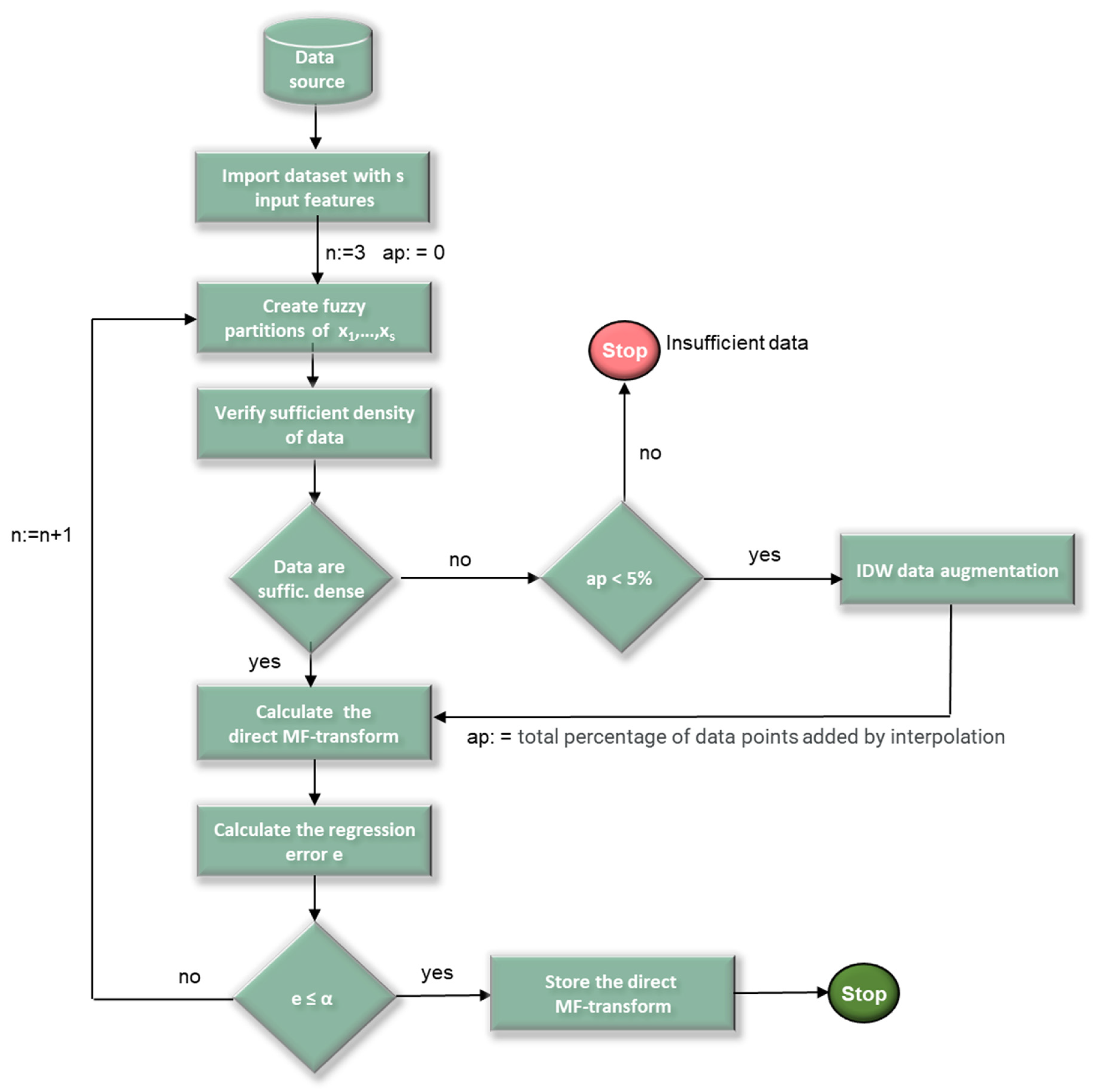
To address this criticality, we propose a variation of the linear regression model based on MF-transforms [7], in which the IDW data interpolation algorithm is used when the data are not dense enough with respect to the fuzzy partitions. The flow diagram in Figure 3 schematizes the IDWMF-Transform method.

Initially, in addition to setting the size of the fuzzy partitions n to 3, the variable ap, which refers to the percentage of new data points, is initialized to 0. If the density of data points is insufficient and the number of added data points does not exceed 5% of the overall cardinality of the data points, then the IDW interpolation method is used to insert new data points in the feature space regions between nodes, where no data points are present, such as the red-lined region in the example in Figure 1.

The IDW data augmentation component uses the IDW interpolation algorithm to add a new point in each of these empty regions to make the new dataset sufficiently dense with respect to the fuzzy partitions. Then, the direct MF-transform and the regression error are calculated; the algorithm ends if the regression error is less or equal to the threshold α; otherwise, the cardinality of the fuzzy partitions is incremented (n = n + 1) and the process is iterated.

The algorithm ends with the error message that the data are not dense enough only if the percentage of new data points added by the IDW interpolator ap exceeds the 5% threshold. Beyond this threshold, the percentage of simulated data points would become non-negligible and would significantly distort the original dataset.

To add a new data point in the space of the features, the data augmentation component uses (10) by considering the K closest sample points of the original dataset and neglecting neighboring data points added via interpolation.

A regression error index can be used to calculate the regression error e. To find the best values of the number of closest data points K and the power parameter p in (10), cross-validation techniques can be adopted.

4. Test and Results

To measure the performance of the IDWMF-transform regression method, a set of tests were performed on well-known time-series datasets.

Let {(x₁₁, x₁₂, …, x_1s, y₁), (x₂₁, x₂₂, …, x_2s, y₂),…,(x_N1, x_N2, …,x_Ns, y_N)} be a dataset of measures. Each data point is given by s numerical input features and one output feature y.

In choosing the regression error index, we avoided adopting scale-dependent regression error measures that cannot be used, as it is necessary that the regression error threshold α is fixed and does not depend on the unit of measurement of the output variable.

The scale-independent symmetric mean absolute percentage error (SMAPE) [27,28] is used to measure the regression error. It is given by:

$$\mathrm{e}=\mathrm{S}\mathrm{M}\mathrm{A}\mathrm{P}\mathrm{E}={\displaystyle \frac{100\%}{\mathrm{N}}}\sum _{\mathrm{j}=1}^{\mathrm{N}}{\displaystyle \frac{2·\left|{\mathrm{f}}_{{\mathrm{n}}_1{\mathrm{n}}_2...{\mathrm{n}}_{\mathrm{s}}}^{\mathrm{F}}\left({\mathrm{x}}_{\mathrm{j}1},{\mathrm{p}}_{\mathrm{j}2},...,{\mathrm{p}}_{\mathrm{j}\mathrm{s}}\right)-{\mathrm{y}}_{\mathrm{j}}\right|}{\left|{\mathrm{f}}_{{\mathrm{n}}_1{\mathrm{n}}_2...{\mathrm{n}}_{\mathrm{s}}}^{\mathrm{F}}\left({\mathrm{x}}_{\mathrm{j}1},{\mathrm{p}}_{\mathrm{j}2},...,{\mathrm{p}}_{\mathrm{j}\mathrm{s}}\right)\right|+\left|{\mathrm{y}}_{\mathrm{j}}\right|}}$$

(13)

SMAPE is expressed in percentage ranges, where a score of 0% indicates a perfect match between the measured and predicted values. With respect to the well-known regression index mean absolute percentage error (MAPE), SMAPE does not have the disadvantage of tending to infinity when the observed value y_j tends to zero; moreover, it is less sensitive to the presence of outliers.

The model was tested using a set of regression datasets in the UCI Machine Learning Repository [29]. In

Table 1. Datasets used in the comparison tests.

Dataset	Data Points	Input Features	Target Feature
Abalone	4177	8	Rings
Auto MPG	398	6	Mpg
Computer hardware	209	9	ERP
Liver disorders	345	5	Drinks
Real estate	414	6	Price

, for each dataset, we give the number of data points, the number of input features, and the name of the target feature.

Comparison tests are performed using Ridge Regression (RR), Huber Regression (HR), Extreme Gradient Boosting (XGB), Random Forest (RF), Support Vector Machine (SVM), K-nearest neighbor (KNN) and MF-transform (MFT).

Each dataset is randomly split into training and test sets, containing, respectively, 80% and 20% of the data. To analyze the performance of each algorithm, for each test set, the regression error indices R², RMSE, MAE, and MAPE were calculated.

In order to set the two IDW parameters, the number of neighborhoods K and the power parameter, for each dataset, a sample consisting of 10% of the data points was randomly extracted. Then, the IDW algorithm was executed multiple times on these sample data to assess the value of the target feature; in each execution, the parameter K varied from 5 to 15 and the parameter p from 1 to 5. The RMSE between the predicted and the measured values was calculated to set the optimal values of the two parameters.

For the sake of brevity, only the tests performed on the Abalone and Real Estate datasets are discussed in detail in Section 4.1 and Section 4.2. The complete comparison results are shown in Section 4.3.

4.1. Comparison Results for Abalone

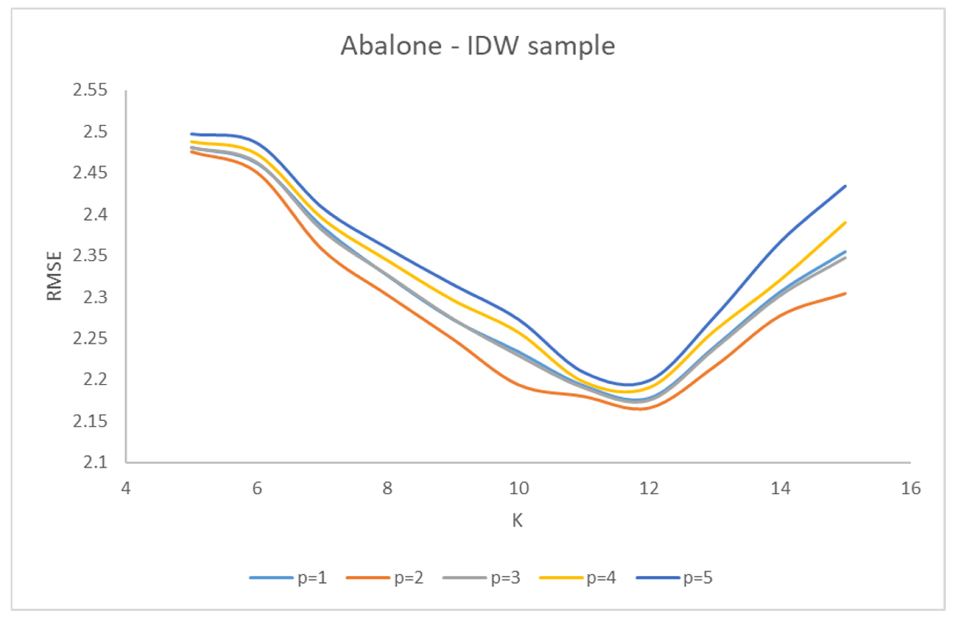
The IDW sample randomly extracted from the dataset is given by 420 data points.

Figure 4 shows the trend of RMSE with respect to k, for various values of p. The RMSE index is minimized for K = 12 and p = 2; then, the values of the two parameters were set, respectively, to 12 and 2.

After randomly splitting the dataset, a training set given by 3342 data points and a test set given by 835 data points are obtained. The eight regression methods are executed on the training set.

MFT and IDW-MFT were executed by setting for the threshold error α = 0.5%. The choice of this value was made on a sample of data points, considering that, for lower threshold values, the reduction obtained in the RMSE is negligible.

Initially, the cardinality of the fuzzy partition n is fixed to three, obtaining a value of SMAPE of 0.823%, which is greater than the threshold value. In the second iteration with n = 4, the SMAPE value is equal to 0.665%, still higher than the threshold. In the third iteration, the MF-transform algorithm terminates because the fuzzy partitions are too fine, and the data are not dense enough with respect to the fuzzy partitions. Instead, the IDW-MFT algorithm, applying the IDW-based data augmentation process, terminates as SMAPE = 0.451, which is lower than the threshold.

Table 2. Abalone—SMAPE values obtained when varying the cardinality of the fuzzy partitions.

n	MFT (%)	IDW-MFT (%)
3	0.823	0.823
4	0.634	0.665
5	/	0.451

shows the MFT obtained executing the two algorithms at each iteration.

Table 3. Abalone—regression results. The best values are shown in bold.

	R2	RMSE	MAE	MAPE
RR	0.540	2.241	1.601	0.161
HR	0.532	2.263	1.610	0.156
XGB	0.473	2.391	1.649	0.170
RF	0.538	2.266	1.580	0.159
SVM	0.538	2.255	1.586	0.158
KNN	0.527	2.269	1.578	0.154
MFT	0.483	2.397	1.672	0.185
IDW-MFT	0.535	2.233	1.554	0.151

shows the value of the regression indices obtained for the Abalone test set. The values obtained when executing MFT are the ones calculated in the second iteration where the cardinality of the fuzzy relations is n = 4.

IDW-MFT exhibited the best performance in terms of RMSE, MAE, and MAPE. The best value of R² was obtained when executing RR. MFT and XGB exhibited the worst performances.

4.2. Comparison Results on Real Estate

Here, we show the results obtained for the Real Estate valuation dataset.

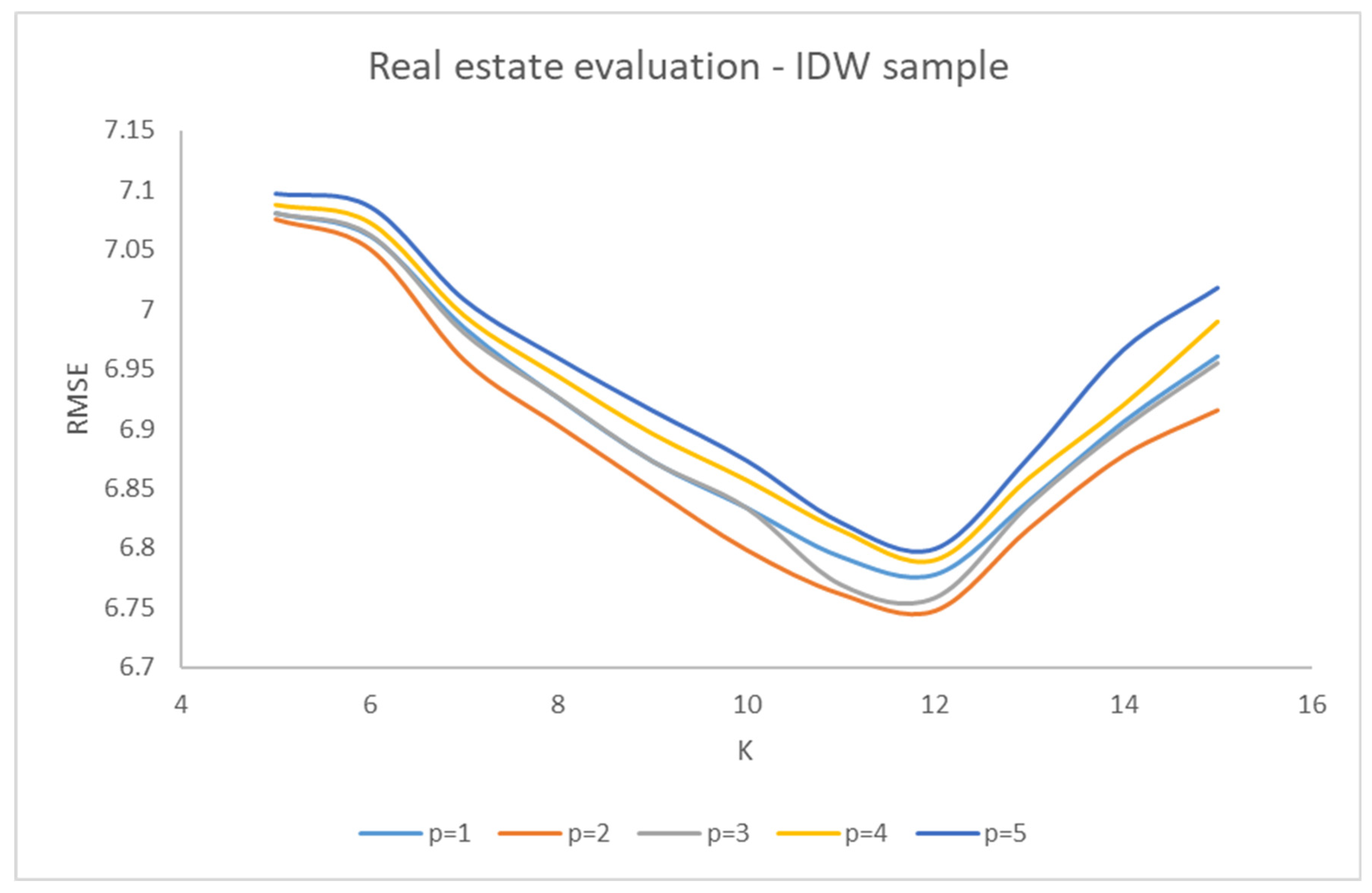
The IDW sample randomly extracted from the dataset is given by 50 data points.

Figure 5 shows the trend of RMSE with respect to k, for various values of p. Even in this case, the minimum values of RMSE are obtained for K = 12 and p = 2.

After randomly splitting the dataset, a training set given by 331 data points and a test set given by 83 data points are obtained. The eight regression methods are executed on the training set.

MFT and IDW-MFT were executed by setting the threshold error α = 0.5%. Initially, the cardinality of the fuzzy partition n is fixed to three, obtaining a value of SMAPE of 0.859%, which is greater than the threshold value. In the next iteration, with n = 4, the MF-transform algorithm terminates because the fuzzy partitions are too fine, and the data are not dense enough with respect to the fuzzy partitions. Instead, the IDW-MFT algorithm, applying the IDW-based data augmentation process, terminates after two iterations, determining a SMAPE error = 0.451, which is lower than the threshold.

Table 4. Real estate—SMAPE values obtained by varying the cardinality of the fuzzy partitions.

n	MFT (%)	IDW-MFT (%)
3	0.859	0.859
4	/	0.638
5	/	0.486

shows the MFT obtained by executing the two algorithms at each iteration.

Table 5. Real estate—regression results.

	R2	RMSE	MAE	MAPE
RR	0.661	7.560	5.589	0.178
HR	0.640	7.774	5.560	0.173
XGB	0.778	5.912	3.952	0.134
RF	0.793	5.833	3.901	0.122
SVM	0.708	6.033	4.328	0.156
KNN	0.649	7.772	5.939	0.185
MFT	0.612	8.065	6.534	0.196
IDW-MFT	0.801	5.778	3.876	0.117

shows the value of the regression indices obtained for the Real Estate test set. The values obtained by executing MFT are those calculated in the first iterations, where the cardinality of the fuzzy relations is n = 3.

IDW-MFT demonstrated the best performance in terms of R², RMSE, MAE, MAPE, and SMAPE. MFT, RR, HR, and KNN exhibited the worst performance.

In the next paragraph, the performance of IDW-MFT with respect to the other regression models for all five UCI Machine Learning datasets are analyzed. The analysis is conducted by evaluating the gain of IDW-MFT with respect to each of the other methods for all four regression measures: R², RMSE, MAE, and MAPE.

4.3. IDW-MFT Gain with Respect to Other Regression Methods

Below, the performance of each regression model against IDW-MFT is compared for all datasets. The comparison is achieved by measuring, for each regression index, the gain of IDW-MFT over the other regression models.

Table 6. R² gain for all datasets.

	RR	HR	XGB	RF	SVM	KNN	MFT
Abalone	−0.009	0.006	0.116	0.006	0.006	0.015	0.097
Auto MPG	0.110	0.154	0.051	0.023	0.059	0.096	0.224
Computer hardware	0.151	0.102	0.098	0.095	0.067	0.089	0.251
Liver disorders	0.077	0.065	0.074	0.081	0.083	0.105	0.149
Real estate	0.175	0.201	0.029	0.010	0.116	0.190	0.236

shows the gain of IDW-MFT for the R² index, given by ${\displaystyle \frac{{\mathrm{R}}_{\mathrm{I}\mathrm{D}\mathrm{W}-\mathrm{M}\mathrm{F}\mathrm{T}}^2-{\mathrm{R}}^2}{{\mathrm{R}}_{\mathrm{I}\mathrm{D}\mathrm{W}-\mathrm{M}\mathrm{F}\mathrm{T}}^2}}$, where R²_IDW-MFT is the value of R² obtained when executing IDW-MFT and R² is the value of R² obtained when executing another model.

Gains in R² values over the other regression models are reported for each of the five datasets, and they fall between 0 and 0.24. IDW-MFT has the highest gain values compared to MFT and KNN.

For the other three indices, the gain is calculated using the formula ${\displaystyle \frac{\mathrm{I}-{\mathrm{I}}_{\mathrm{I}\mathrm{D}\mathrm{W}-\mathrm{M}\mathrm{F}\mathrm{T}}}{{\mathrm{I}}_{\mathrm{I}\mathrm{D}\mathrm{W}-\mathrm{M}\mathrm{F}\mathrm{T}}}}$, where I_IDW-MFT is the value of the index obtained when executing IDW-MFT, and I is the value of the index obtained when executing another model.

The IDW-MFT gain for the RMSE index is displayed in

Table 7. RMSE gain for all datasets.

	RR	HR	XGB	RF	SVM	KNN	MFT
Abalone	0.004	0.013	0.071	0.015	0.010	0.016	0.073
Auto MPG	0.058	0.057	0.065	0.044	0.043	0.062	0.112
Computer hardware	0.147	0.122	0.096	0.082	0.069	0.101	0.180
Liver disorders	0.091	0.086	0.090	0.097	0.102	0.123	0.194
Real estate	0.308	0.345	0.023	0.010	0.044	0.345	0.396

. Significant RMSE gains were observed for all regression models for the datasets of computer hardware and liver disorders, for all regression models other than XGB and RF for the Real Estate dataset, and for XGB for the Abalone dataset and HR for the Auto MPG dataset. The increase fluctuates between 0.07 and 0.4 in relation to MFT.

Table 8. MAE gain for all datasets.

	RR	HR	XGB	RF	SVM	KNN	MFT
Abalone	0.030	0.036	0.061	0.017	0.021	0.015	0.076
Auto MPG	0.053	0.099	0.086	0.027	0.033	0.060	0.163
Computer hardware	0.092	0.096	0.085	0.069	0.057	0.083	0.231
Liver disorders	0.221	0.177	0.183	0.084	0.081	0.128	0.564
Real estate	0.442	0.434	0.020	0.006	0.117	0.532	0.686

displays the improvement shown by IDW-MFT for the MAE metric. Across all five datasets, the improvements in MAE compared to the other regression models vary from 0 to 0.69. The maximum gain values are seen with respect to MFT, HR, and KNN.

The gain of IDW-MFT for the MAPE index is displayed in

Table 9. MAPE gain for all datasets.

	RR	HR	XGB	RF	SVM	KNN	MFT
Abalone	0.066	0.033	0.126	0.053	0.046	0.020	0.225
Auto MPG	0.092	0.131	0.127	0.073	0.068	0.094	0.387
Computer hardware	0.115	0.147	0.096	0.078	0.070	0.093	0.432
Liver disorders	0.268	0.236	0.424	0.131	0.073	0.155	0.419
Real estate	0.521	0.479	0.145	0.043	0.333	0.581	0.675

. The MAPE gains over the other regression models for each of the five datasets fall between 0 and 0.68. IDW-MFT has the highest gain values over MFT, HR, and KNN.

These results highlight that IDW-MFT exhibits, in general, better performance than other well-known regression models, in terms of regression error reduction. For all datasets used in the tests, gains compared to other regression models are recorded for all five error measures.

5. Conclusions

A variation of the Multidimensional F-transform regression method based on the IDW interpolator is proposed in this study. IDW is applied in a data augmentation process performed at each iteration in the regions of the feature space with insufficient data density concerning the fuzzy partitions. This process overcomes the performance limitations of MF-transform, which cannot be used when sufficient data density concerning the fuzzy partitions is not respected.

The results of the comparative tests, both with MF-transform and with other well-known regression models, showed that the IDW-MF-transform exhibits better regression performance than MF-transform and the other regression methods for all five datasets used in the tests. In the future, we intend to perform further tests on many datasets of different cardinalities and sizes to analyze the performance of the model when the number of features and data points varies. Furthermore, a future evolution of the research will be directed towards adapting the method to manage massive datasets.