Article

Generator-Level Transient Stability Assessment in Power System Based on Graph Deep Learning with Sparse Hybrid Pooling

1
CSG Energy Development Research Institute Co., Ltd., Guangzhou 510663, China
2
School of Electric Power, South China University of Technology, Guangzhou 510641, China
3
Guangdong Provincial Key Laboratory of Intelligent Operation and Control for New Energy Power System, Guangzhou 510663, China
4
CSG Power Dispatching and Control Center, Guangzhou 510663, China
5
CSG Electric Power Research Institute Co., Ltd., Guangzhou 510663, China
*
Author to whom correspondence should be addressed.
Electronics 2025, 14(6), 1180; https://doi.org/10.3390/electronics14061180
Submission received: 26 January 2025 / Revised: 17 February 2025 / Accepted: 26 February 2025 / Published: 17 March 2025

Abstract

:
Aimed at increasingly challenging operation conditions in modern power systems, online pre-fault transient stability assessment (TSA) acts as a significant tool to detect latent stability risks and provide abundant generator-level information for preventive controls. Distinguished from “system-level” to describe terms concerning the whole system, here “generator-level” describes those concerning a generator. Due to poor topology-related expressive power, existing deep learning-based TSA methods can hardly predict generator-level stability indexes, unless they adopt the generator dynamics during and after faults by time-domain simulation (TDS) as the model input. This makes it difficult to fully leverage the speed advantages of deep learning. In this paper, we propose a generator-level TSA (GTSA) scheme based on topology-oriented graph deep learning which no longer requires time-domain simulation to provide the dynamic features. It integrates two modules to extract the network-dominated interaction trends from only the steady-state information. A sparse Edge Contraction-based Attention Pooling (ECAP) scheme is designed to dynamically simplify the network structure by feature aggregation, where the generator-specific information and key area features are kept. A Global Attention Pooling (GAP) module works to generate the interaction features among generators across the system. Hence, the constructed ECAP&GAP-GTSA scheme can not only output the system stability category but also provide the dominant generators and inter-generator oscillation severity. The performance as well as interpretability and generalization of our scheme are validated on the IEEE 39-bus system and the IEEE 300-bus system under various operation topologies and generator scales. The averaging inference time of a sample on the IEEE 39-bus system and IEEE 300-bus system is merely 1/671 and 1/149 of that of TDS, while the accuracy reaches about 99%.

1. Introduction

1.1. Literature Review and Motivation

The increasing penetration of renewable generation as well as the ever-growing demand for electrical power lead to power system operation much closer to stability boundaries [1]. In such a context, online pre-fault transient stability assessment (TSA) becomes a fundamental requirement to periodically (15 min in general) discriminate the instability risks based on pre-defined contingencies. With the increasing converter-interfaced power sources in today’s power systems, time-domain simulation (TDS) struggles to meet the demands of much smaller time steps, more complex models and shorter TSA periods. Rapid online TSA demands make model-free machine learning (ML) an increasingly popular choice for TSA [2,3,4,5,6,7,8], especially those not relying on the TDS since they can provide faster response and sensitivity information [5,6,7,8]. Encouraging works have been reported to promote the feasibility of TDS-free TSA schemes based on deep learning models [9,10,11,12,13]. The network topology is represented by nonparametric one-hot encoding [9] or graph convolutions [10,11], which enhances the generalization of the TSA models to various topologies or contingencies. In the plain topology learning structure, the task-specific network faces a large training burden in real-world systems and no longer works under a new system scale, whose input size is proportional to the input system scale. Graph pooling helps adapt TSA models to system-scale variations [12,13] in case of the system-level stability status classification or index regression. The global pooling structure with max/mean pooling [12] reduces the scale of nodes thoroughly and represents them by a fixed-size vector. The expressive power of this scale reduction is so poor that the model has to preserve the effective information through an ensemble mechanism. Inspired by the community nature, a hierarchical pooling structure with node cluster-based pooling [13] enhances the function by transforming an input system into minor diverse clusters. Note that both the scale of the clusters and their representations are pre-defined and unchanged.
In power system practice, operators usually need more abundant TSA information, such as the dominant generators or instability modes, etc. These guide the preventive controls like power adjustment on the generators strongly related to system instability. Technically, it is challenging for the ML-based TSA models such that it is denoted as generator-level transient stability assessment (GTSA) to distinguish itself from the system-level assessment. Currently, few TDS-free data-driven GTSA schemes are available. The ML-based GTSA schemes highly rely on the fault-on and post-fault dynamics as their input features, while these can be only derived from TDS when applied to online pre-fault TSA. With these dynamic inputs, the support vector machine (SVM) or artificial neural network (ANN) is developed to predict the system instability modes in [14,15,16], which is modeled as a multi-class classification problem with each pattern linked to a class label. Mazhari et al. [17] label the stability status of each generator pair and set up a random forest (RF) model for the classification.
Deep learning (DL) techniques such as convolutional neural network (CNN), long short-term memory (LSTM) [18] and Transformer map input vectors to more expressive features through convolution or attention operation. The generator dynamics are organized into a heatmap and fed to CNN [19] or Vision Transformer (ViT) [20] that achieves feature aggregation for better performance of the succeeding task-specific shallow networks. Zhu et al. [21] introduce a spatial-temporal graph learning model that operates on generator dynamics according to an adjacency matrix representing the network spatial correlations among the generator buses. Huang et al. [22] propose a recurrent graph convolutional network (RGCN) to integrate the dynamics of the entire system.
Without TDS to translate the fault impacts and network-dominated generator interactions into dynamic features, it is of great necessity for the TDS-free GTSA schemes to tackle three significant challenges:
(1) The DL-based hierarchical feature aggregation should properly integrate the network-dominated interaction trends among generators.
(2) The generator-specific information should be kept such that the grouping-related features can be extracted in the high-dimensional feature space.
(3) It is important to design appropriate generator-level stability indexes so as to pilot the training process during back-propagation.
Though graph pooling methods in TSA can address the hierarchical features, they fail under generator-scale changes, especially unseen generators that bring new labels. The inter-node differences are not available [12], or the expressive power of generator representations is weakened when the generator nodes and other ones are merged in clusters [13]. This motivates us to design a new graph pooling method.

1.2. Contribution in This Paper

To overcome existing gaps, a novel graph deep learning-centered scheme is designed to realize the TDS-free GTSA. The Edge Contraction-based Attention Pooling (ECAP) proposed in [23] is adopted to produce the coarsened graph representation of a large power network. A Global Attention Pooling (GAP) module is designed to acquire the generator-level feature representations. Finally, two downstream networks, i.e., the dominant generator predictor (DGP) and the generator perturbation predictor (GPP), are shared by all the generators and work to yield dominant generators and post-fault generator severity (i.e., a metric to reflect the relative motion compared with the reference generator or bus).
The main contributions are summarized as follows:
(1) The sparse graph pooling ECAP layers merge nodes dynamically and differentially without significant information loss on generator interactions.
(2) The GAP module produces attention sequences on relative interaction (e.g., angle oscillations) among the remaining generators and coarsened nodes. Each attention sequence instructs a generator to aggregate global information into its low-dimensional representation.
(3) Based on hybrid poolings and well-designed downstream networks, the proposed ECAP&GAP-GTSA scheme can predict the dominant generators and the inter-generator oscillation severity independent from TDS for dynamic features. Moreover, there is an in-depth interpretation of the obtained attention sequences through the cross-comparison with the TDS results in the case studies.
The rest of the paper is organized as follows. Section 2 introduces the motivation for the data-driven GTSA scheme. Section 3 provides an overview on the proposed ECAP&GAP-GTSA scheme, while Section 4 presents the detailed designs. Section 5 demonstrates the training and evaluation of ECAP&GAP-GTSA. Case studies are conducted on the IEEE 39-bus system and IEEE 300-bus system in Section 6. Finally, conclusions and discussions are available in Section 7 and Section 8.

2. The Motivation for the Data-Driven GTSA Scheme

2.1. The Underlying Design Philosophy of GTSA

Although generators are undoubtedly critical in TSA, the network topology and power flow play a complex and important role in the post-fault dynamic of generator rotors, which must be considered in a TDS-free GTSA scheme.
In a real-world power system, non-generator nodes make up the vast majority in terms of quantity. Therefore, a GTSA scheme should emphasize the relative motions among generators and aim to aggregate stability information.
To address the above technical challenges, TDS simulates the post-fault dynamics based on the mathematical power system model described by differential algebraic equations. In case of transient instability, the leading generator(s) with distinguished angles and rotor speeds are denoted as the dominant generators [24]. Figure 1 demonstrates a case study on the IEEE 39-bus system in Figure 2 to highlight the influence of slight topology change on the behavior of the dominant generators. Note that there are 39 buses, 10 generators, 19 loads and 46 transmission lines. The balancing generator is connected to bus 39.
The dominant generators are annotated with gray circles in Figure 1b,d. t u , max denotes the instability time of the most leading one. The fault impact is reflected by absolute voltage drop Δ U at fault occurrence and the strong color intensity in Figure 1a,c.
A nearly causal correlation between the fault impacts (on the left) and the generator swing curves (on the right) can be observed. It appears that the leading generators are situated in areas where there are severe voltage drops. Additionally, even minor changes to the network topology can have a significant impact on stability status. Compare two cases under an instantaneous fault (Figure 1a,b) or a permanent fault (Figure 1c,d) on bus 02-bus 25. Their only difference is whether bus 02-bus 25 remain connected or is disconnected after the fault, where the system is stable in the former case but loses synchronization in the latter case.
Above analysis prompts three principles for the design of the GTSA scheme as follows:
I. The voltage drop and power impacts resulting from a fault are critical features to be considered. Furthermore, the features of the generators should be distinguished from those of the grid nodes in the feature aggregation modules.
II. Special designs are required to identify the generator grouping mode during oscillation, where the sparse grid-like interconnection among generators may play a crucial role.
III. In order to predict generator-level stability indexes, it is crucial to extract a global feature representation for each generator that incorporates its interactions with the rest of the network nodes.
More informative generator-level stability labels may benefit model training and parameter optimization.

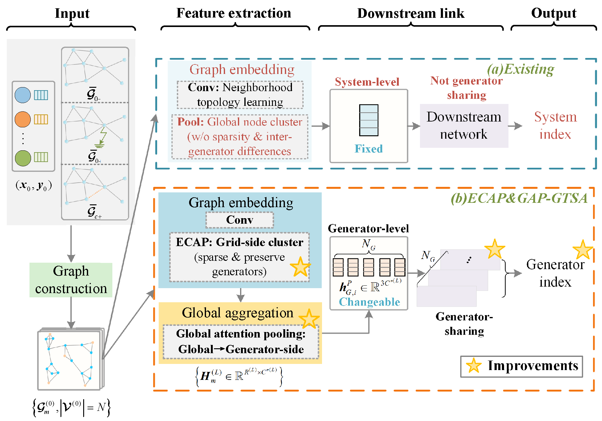
2.2. Related Works and the Proposed Improvements

The graph learning schemes presented in [12,13] have proven effective for system-level TSA using TDS-free input features and graph embedding on network topology. Building upon the model proposed in [13], several new designs that adhere to the aforementioned principles are introduced in order to achieve our GTSA.
Figure 3 compares the proposed model with the model in [13]. They have the same input feature designs. In an N-bus system, there are steady-state variables ( x 0 , y 0 ) N and parameterized topologies G ¯ m , m = 0 , 0 + , c + . Here, x 0 , y 0 refer to state variables and algebraic variables. ∝ denotes proportionality. The input features consist of a mathematical graph set G m ( 0 ) , V ( 0 ) = N , m = 1 , 2 , 3 , where V ( 0 ) contains the input nodes. Each graph consists of a node feature matrix X m R N × 5 and an adjacency matrix A m R N × N . The row-wise feature vector X m ( i , : ) covers voltage amplitude, the active and reactive power flow to the loads, and the active and reactive power injected by generators. Note that X 2 and A 3 involve the impact of fault occurrence and clearance.
There are two blocks in the right part of Figure 3. The upper block denoted as (a) shows the structure of the model in [13], whose graph embedding module incorporates the graph convolution (“Conv”) with the pooling (“Pool”) layers for topology addressing and scale reduction. Convolution enables efficient learning of neighborhood topology, while the global node cluster-based pooling generates dense topology and clusters. However, such a scale reduction approach neglects the impact of generators’ interconnection topology. In addition, a single downstream network adapts its parameters to the system, hindering the acquisition of stability characteristics for each generator in a flexible manner. Therefore, only the system stability index can be predicted by the scheme.
The lower block denoted as (b) is the proposed ECAP&GAP-GTSA scheme. The ECAP in the graph embedding generates sparse topologies and differentially clusters similar grid-side nodes, with the generator nodes always preserved. Then, a novel global aggregation is proposed, where the global information regarding the grid-side coarsened nodes and the generators is aggregated for each generator via the GAP. N G parameter-sharing downstream networks predict the generator-level stability. Furthermore, well-designed generator-level stability indexes are adopted for the training and prediction.

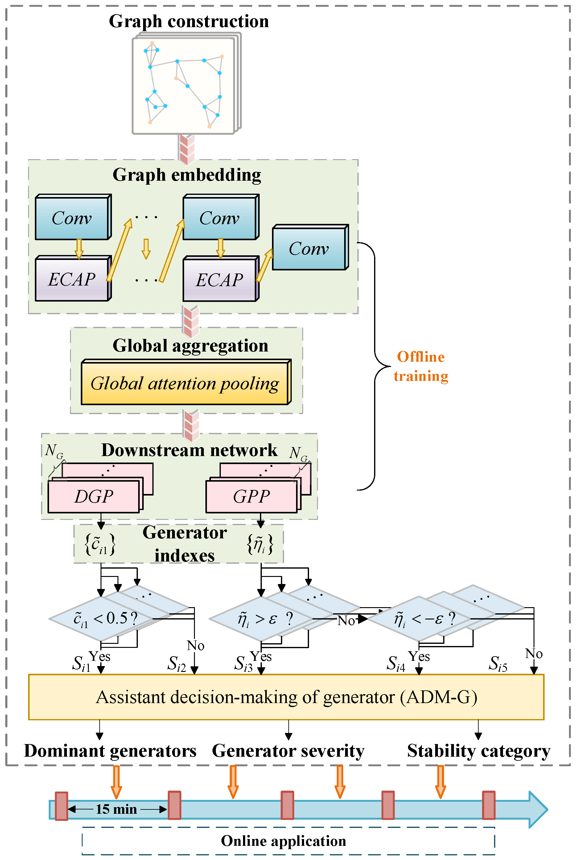
3. The Scheme Overview of ECAP &GAP-GTSA

The modules of ECAP&GAP-GTSA scheme are illustrated in Figure 4. At online stage, DGP and GPP scan all the generator representations for generator indexes c ˜ i 1 and η ˜ i . An assistant decision-making of generator (ADM-G) handles output pairs ( c ˜ i 1 , η ˜ i ) such that we can acquire the final dominant generator set G ˜ d , generator severity vector η ˜ o and system-level stability category c ˜ G 2 S . The design details are explained in the following sections.

4. Detailed Designs of the ECAP &GAP-GTSA

4.1. The Generator-Level Stability Indexes

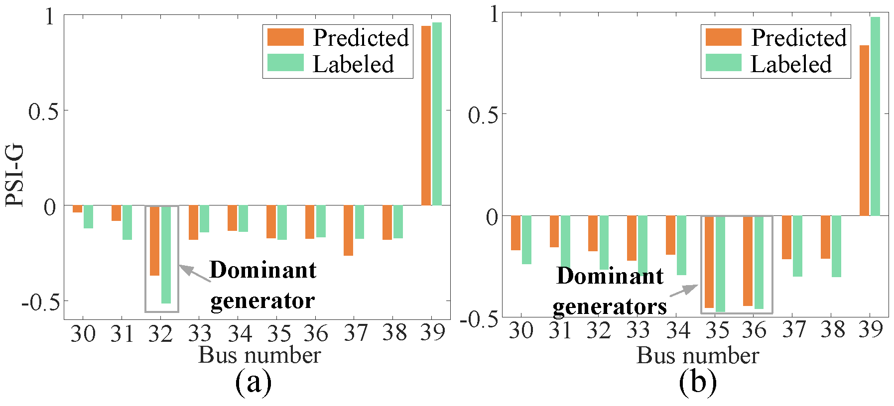
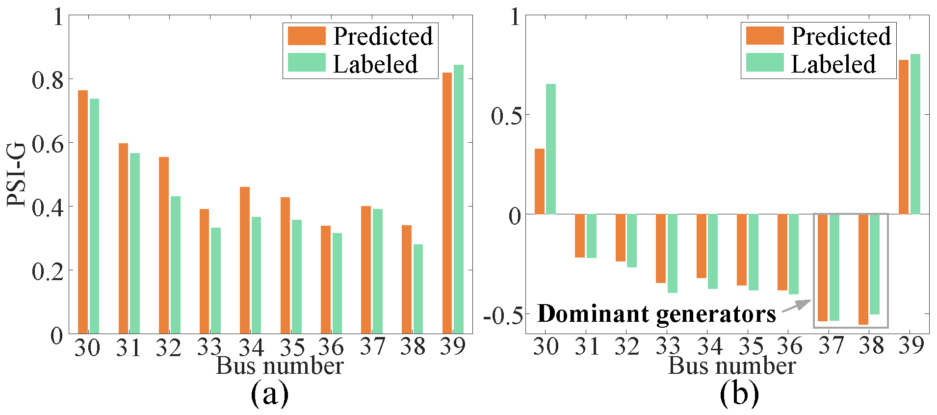
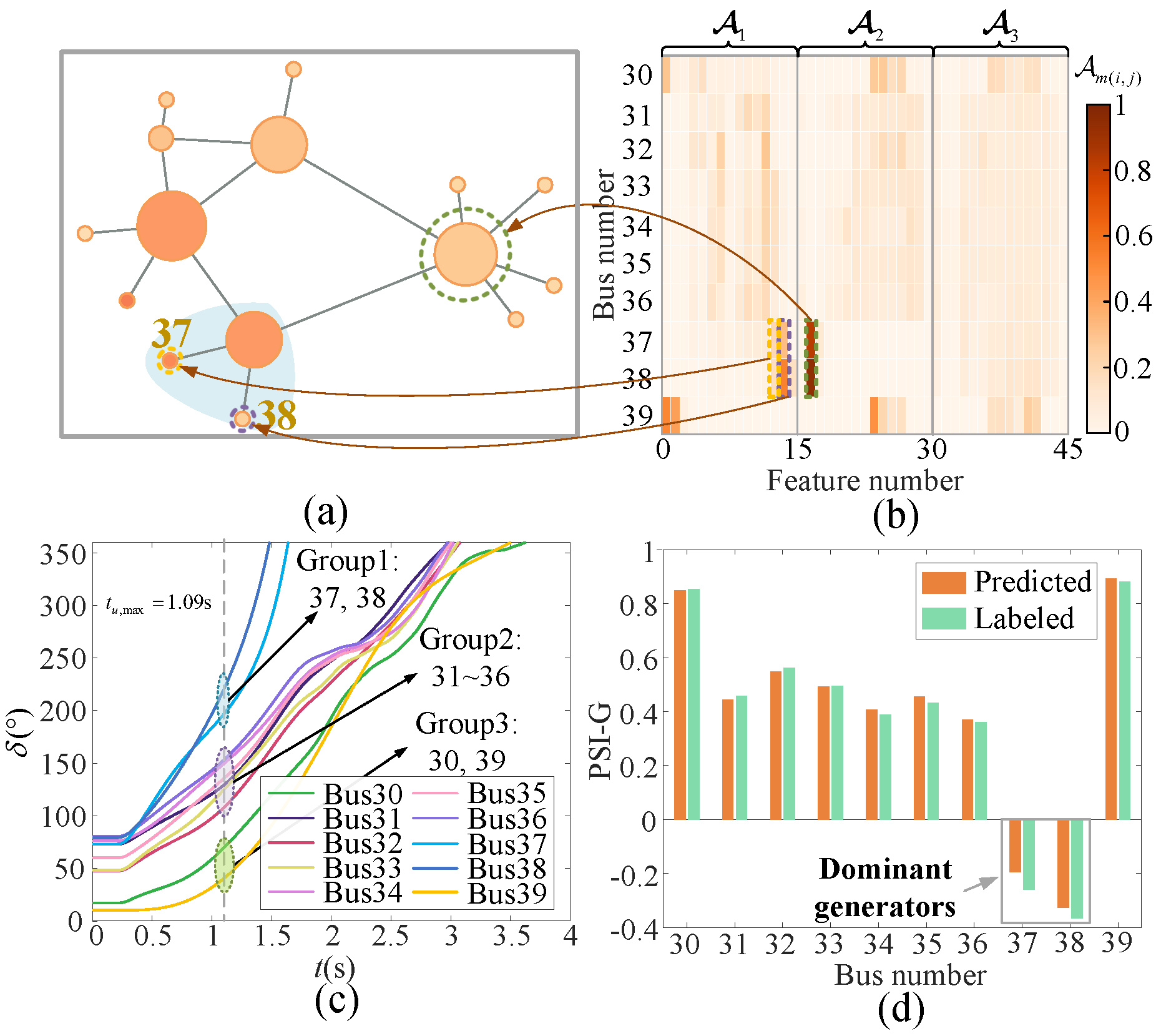
4.1.1. Dominant Generators

The most leading generator is chosen at first and then the other dominant generators with similar trajectories are discovered by a cluster approach.
Specifically, given the angle of the i t h generator δ i ( t ) at the moment t, the maximum angle difference is Δ δ ( t ) = max i , j δ i ( t ) δ j ( t ) . The moment t = t u , max is recorded when Δ δ ( t ) exceeds 180 the first time. At this moment, the most leading generator refers to that with the largest angle. Assume a time window t t h , the similarity between two angle trajectories is expressed as
ρ ( i , j ) = t = t u , max t t h t = t u , max δ i ( t ) δ j ( t ) δ i ( t ) δ j ( t ) max i δ i ( t ) max i δ i ( t ) 2
Then, affinity propagation (AP) cluster [25] is carried out on the similarity matrix ρ , where the diagonal elements ρ ( i , i ) are set as the median of all the elements. Note that only top N d generators are chosen according to their angles in a large-scale system. Several generator groups, each of which involves generators with similar dynamics, are available. The dominant generators are exactly covered in the group (described as a set G d ) that includes the most leading generator. G d is then transformed into a binary vector c to describe dominant statuses, whose element c i ( i G ) is as follows:
c i = 0 i G d 1 i G d

4.1.2. Generator Severity

The generator severity describes the stability level of each generator. It provides information about generator grouping since those with similar indexes tend to keep coherency, which is beneficial for more comprehensive preventive controls and less miss of alarm.
Specifically, according to the piece transient stability index in [11], instability time t u , i ( i G u ) and the maximum relative angle difference Δ δ r , i , max are adopted to describe the severity of unstable and stable generators. Here, the unstable generator set G u is acquired as follows [17]:
Define G , N G as the generator set and its scale. δ i denotes the angle of the i t h ( i G ) generator, while Δ δ ( t ) = δ i δ j denotes the absolute angle difference between the i t h and j t h generator. From t = 0 , it calculates the maximum Δ δ ( t ) at each step and the corresponding generator pair G p = { i , j δ i > δ j } . If Δ δ ( t ) max exceed the pre-defined threshold exactly at t = t u , i , then the instability time t u , i describes the stability level of the i t h generator that belongs to the accelerating unstable generator set G u . Let G = G i and repeat the above calculation until all the stability levels of the unstable generators are acquired. Here, ∖ refers to the deletion of the generator i from the set G .
Δ δ r , i , max is related to the chosen reference bus. Considering that the balancing generator could vary under different operation conditions, the voltage phase is selected at a key bus with a low probability of shutdown. Assume its TDS curves θ r e f ( t ) , Δ δ r , i , max are derived as
Δ δ r , i , max = max t ( δ i ( t ) θ r e f ( t ) )
Then, our piece transient stability index of the generator (PSI-G) is expressed as
PSI - G i = min ( C δ , max Δ δ r , i , max C δ , max + Δ δ r , i , max + ε , 1 ) i G u ( a ) max ( σ ( t u , i + τ ) 1 ε , 1 ) i G u ( b )
Here, C δ , max is a constant that represents the maximum of all Δ δ r , i , max in the history data. t u , i = ( t u , i μ u ) / ξ u refers to the normalized instability time, where μ u , ξ u are mean and variance of all t u , i in the history data. The modulation factor τ translates the outliers to the saturation region of the sigmoid function σ ( · ) . The threshold ε forms an uncertain area ε , ε to discover the critical generators.

4.2. Construction of Feature Extraction in Feed-Forward Propagation

Two key links of the proposed scheme are the hybrid ECAP and GAP, where ECAP satisfies principles I and II proposed in Section 2.1, while GAP generates N G generator representations to realize principle III.
It is necessary to determine the pooling-convolution structure in graph embedding. Two typical structures have been proposed. As Figure 5, one is coupled [13] while the other is decoupled [26]. The difference lies in whether pooling affects convolution. Assume a topology derived from the IEEE 39-bus system with bus 31 and bus 32 as generators. During post-fault stages, two generators interact through the network. Graph embedding is expected to cover this nature, i.e., perturbation messages at bus 31 result in feature changes at bus 32.
Suppose there is no loss during the perturbation message passing along the directional path from bus 31 to bus 32. The decoupled one needs nine “Conv” layers while the coupled one needs only four ones since it allows message passing between high-order neighbors in the input graphs. All the convolutions in the former structure operate on the same topology, whereas those in the latter one operate on different (coarsened) graphs to extract various spatiotemporal characteristics of a hierarchical power system, which helps guide and improve poolings. Though message paths are usually diverse and over-smooth, which might cause message loss in real cases, it is still inferred that the coupled structure benefits from more sufficient message passing or convolutions. It is preferable to promote topology-relate operations in large-scale systems with high requirements on interaction feature extraction.

4.3. ECAP

As Figure 5b, the l t h ( l 0 ) block in graph embedding contains a “Conv” and an ECAP layer, except for the last block with merely a “Conv”. The operations in “Conv” is consistent with [13], whose output H m ( l ) R R ( l ) × C ( l ) is fed into ECAP. Here, R ( l ) , C ( l ) denote the (coarsened) system scale and feature dimension. ECAP contracts edges appropriately before the node sets V q c ( l + 1 ) to be merged are available. A set corresponds to a physical area and forms a node V q ( l + 1 ) in the new graph, i.e., an area node with synthetic features.
Note that in the input graph, h m i ( l ) denotes the i t h row vector of H m ( l ) while X m ( i , : ) ( l ) carries original features of the i t h node. There is X m ( i , : ) ( 0 ) = X m ( i , : ) when l = 0 without pooling. When l > 0 , define X m ( i , j ) ( l ) = V i V q c ( l ) X m ( i , j ) ( l 1 ) based on the area V i c ( l ) to generate the i t h area node. The operation ⊕ follows the settings below. It averages voltage amplitudes and sums powers as area-level voltage and power injection.
Figure 6 presents the operation procedure in the ECAP. The pooling template in block (a), the edge scoring in block (b) and the node aggregation in block (c) are discussed in detail.

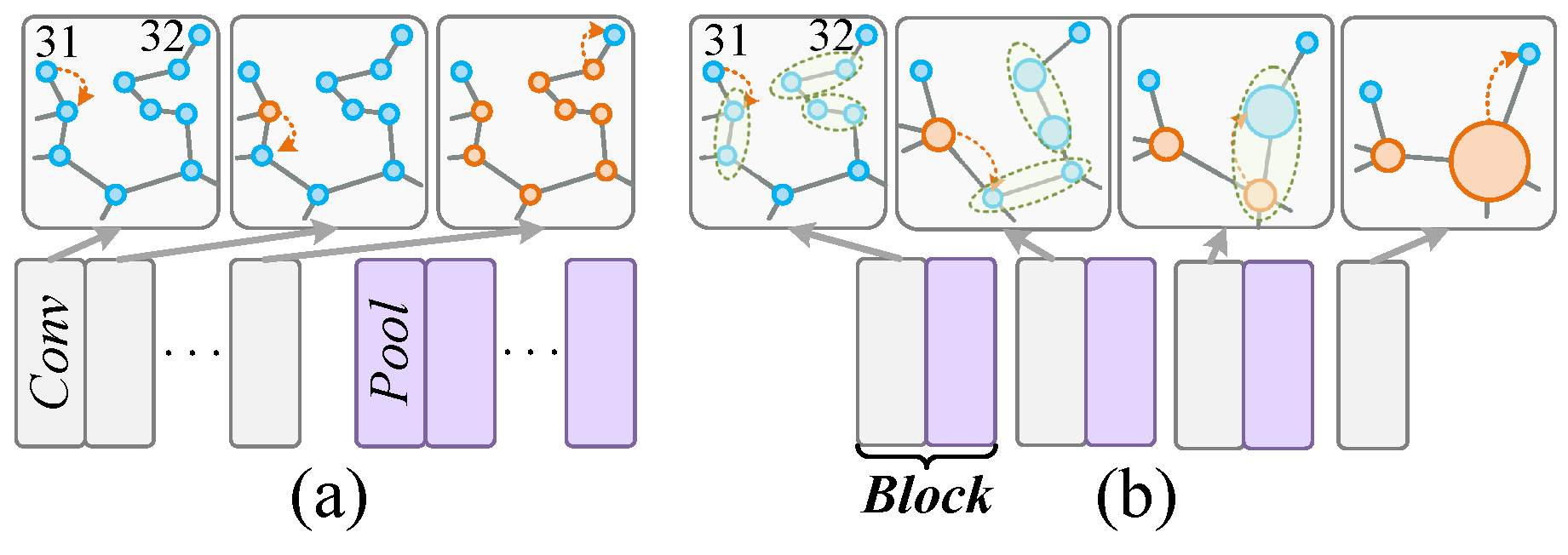
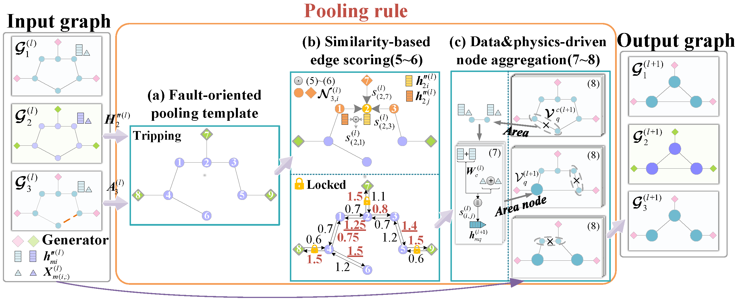
4.3.1. The Pooling Template

The pooling template is designed according to Principle I in Section 2.1. The pooling template involves H 2 ( l ) and A 3 ( l ) . As Figure 6 block (a), H 2 ( l ) carries information of transient impacts (or their coarsened version) caused by fault occurrence, while A 3 ( l ) storages the (coarsened) topology characteristics concerning the clearing mode.
Focusing on the faulted line highlighted by the red dotted edge, it indicates how the fault information is reflected during node mergence through cases under two clearing modes.
When the line tripping does not occur, the buses at both sides of the faulted line power are connected throughout the transient process. Hence, the highlighted edge is allowed to be contracted. The transient impacts are implicitly recorded in the area node features and guide the mergence rule.
If a permanent fault is cleared by line tripping, the highlighted edge (5–6) disappears. The nodes at both sides or the area nodes containing them cannot be merged. In addition to node features, the impacts of fault location and line tripping are both explicitly embedded into the coarsened topologies.
In this way, the pooling template refers to the uniform expressive mergence rule for graphs such that the node alignment does not need to be addressed.

4.3.2. The Pooling Operation
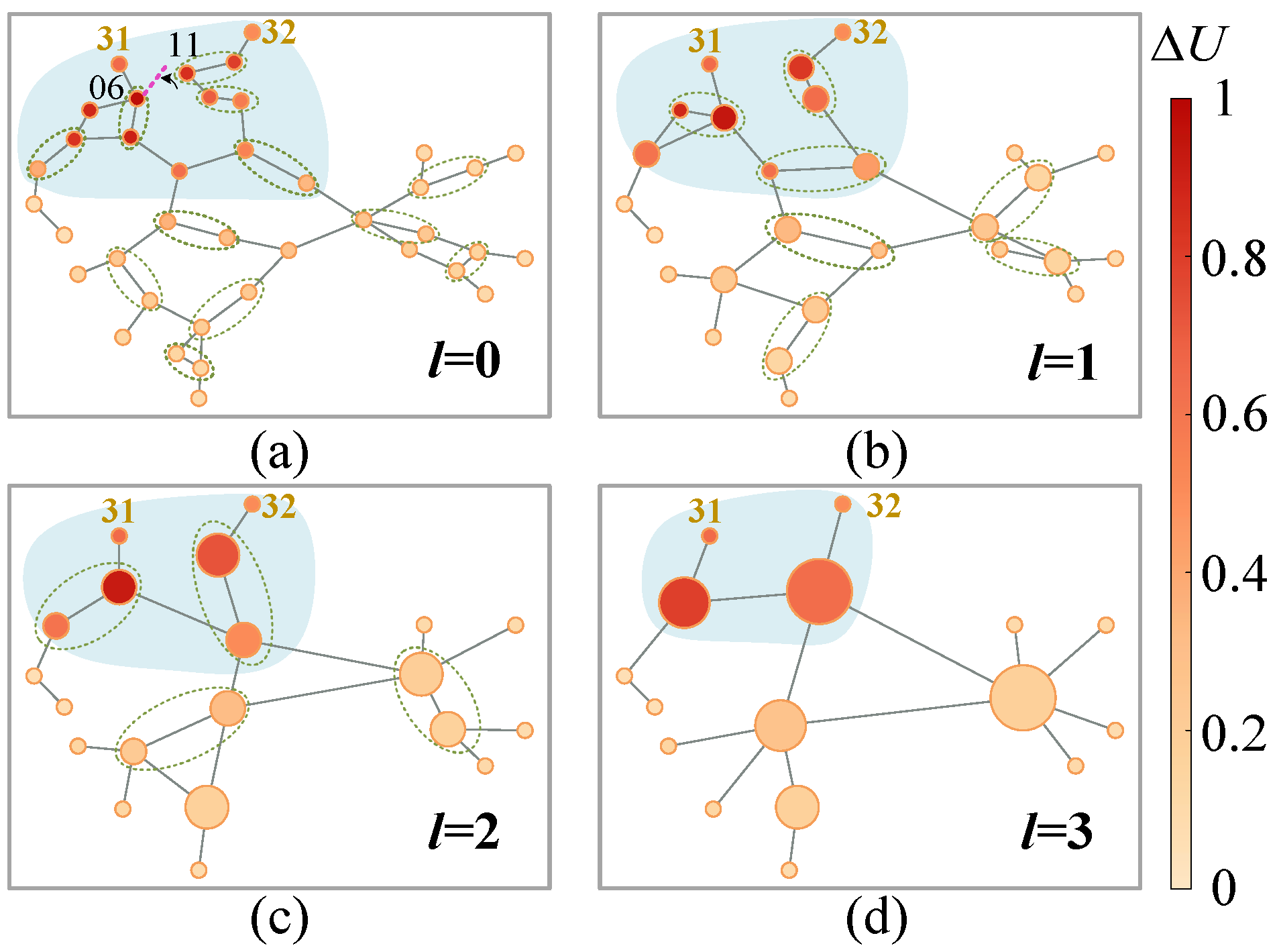
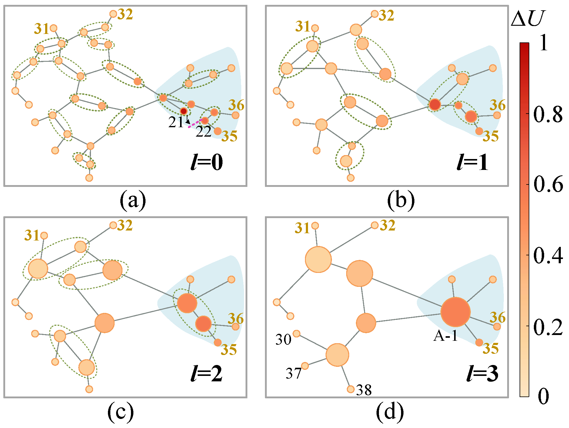
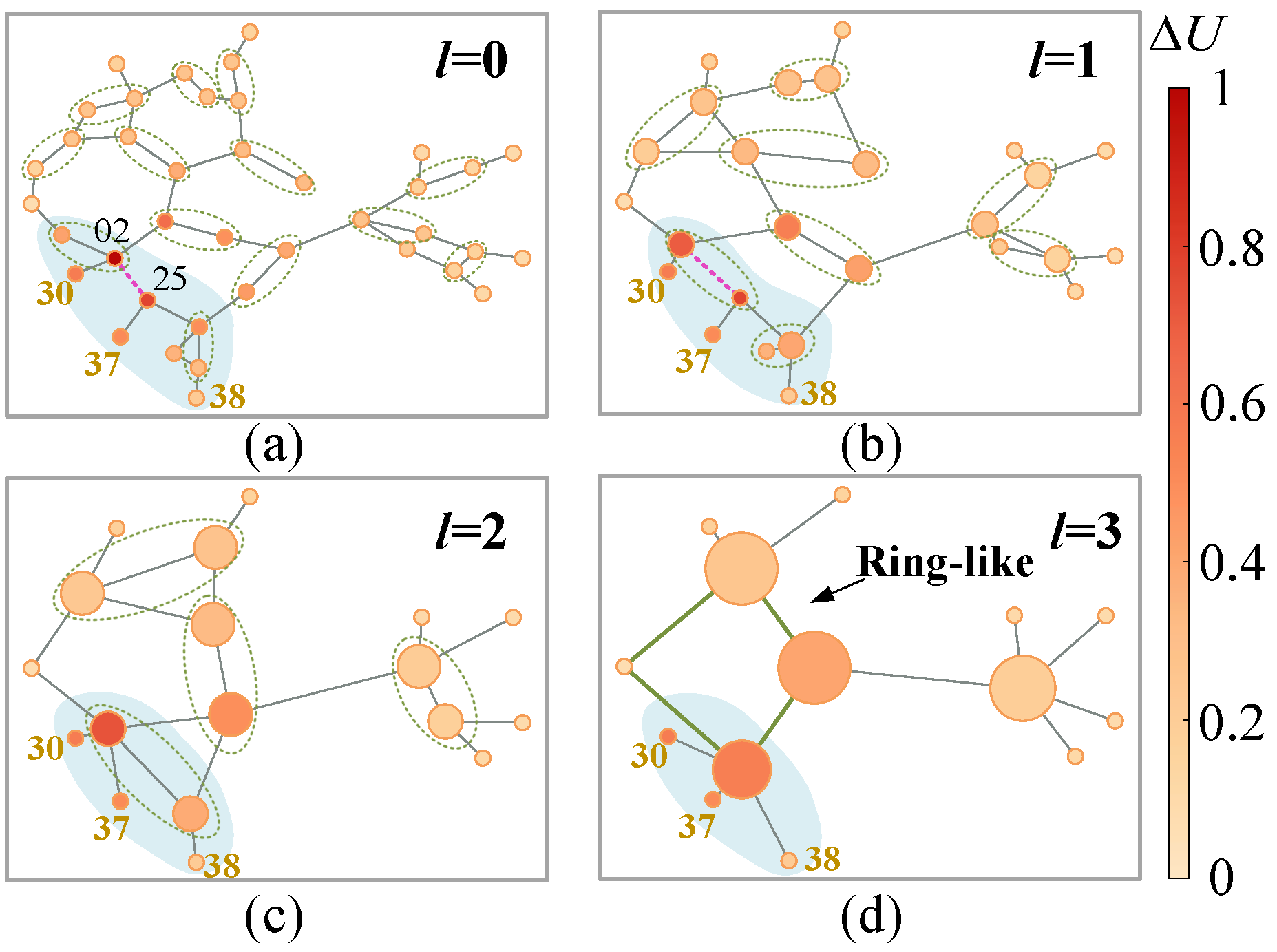
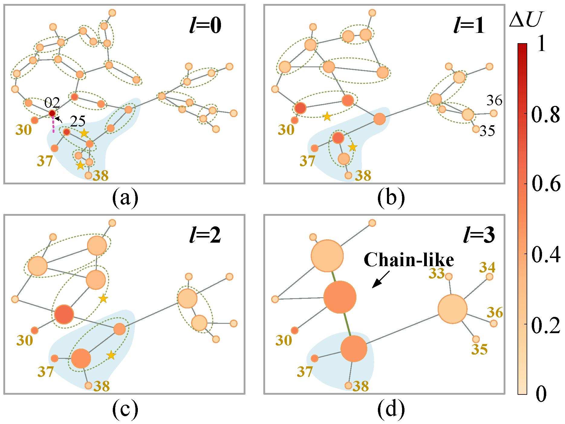
The following three problems are waiting for a solution through the ECAP design.
  • The edge contraction criterion
    To preserve the inter-node difference as much as possible, node similarity is preferred as the edge contraction criterion. The first-order neighborhood representations h 2 i ( l ) involving continuous attributes and discrete topologies are available from convolutions. An attention mechanism is required [23]:
    α e , k ( i , j ) ( l ) = σ leaky h 2 i ( l ) W e , k ( l ) · h 2 j ( l ) W e , k ( l ) C ( l ) , j N 3 , i ( l )
    where h 2 i ( l ) denotes the i t h row of H 2 ( l ) and the first-order neighborhood set N 3 , i ( l ) comes from A 3 ( l ) . Hence, the attention coefficients α e , k ( i , j ) ( l ) vary as the pooling template changes, which meets the principle I. σ leaky refers to the LeakyReLu function. W e , k ( l ) R C ( l ) × C ( l ) refers to the parameter matrix of k t h attention head. Diehl et al. [23] indicate that the mean of edge scores s ( i , j ) ( l ) should be close to 1 considering the numerical stability of model training. Specifically, the node similarity is quantified by the edge score
    s ( i , j ) ( l ) = 0.5 + softmax j N 3 , i ( l ) k α e , k ( i , j ) ( l ) k α e , k ( i , j ) ( l ) K e K e
    Here, K e edge attention coefficients α e , k ( i , j ) ( l ) are averaged. Note that s ( i , j ) ( l ) s ( j , i ) ( l ) is common after the softmax operation and the mergence is actually directional. Define s ( i , j ) ( l ) as the edge score from node V j ( l ) to node V i ( l ) . Only consider unidirectional mergence along the one of larger value is considered, i.e, if s ( i , j ) ( l ) > s ( j , i ) ( l ) , the smaller s ( j , i ) ( l ) is ignored during mergence. It means the V i ( l ) is combined to V j ( l ) along the edge ( V i ( l ) , V j ( l ) ) . In Figure 6b, V 2 ( l ) obtains its neighborhood edge scores through (7)∼(8) and the scores highlighted in red are left.
    Generally, the areas are produced according to s ( i , j ) ( l ) from high to low. Extra limits are also required considering the nature of the power system. On the one hand, generators are usually connected to the main network through substation branches. Edges derived from such branches rank the highest after (7)∼(8), which might cause all the key generators to be merged during the first pooling. This violates the requirement in principle I. Hence, generators and relevant edges are “locked”, i.e., independent from the pooling. On the other, an area node should share the same physical meaning with the area. It means a node can only be assigned to an area during an ECAP. Two areas or an area and a node are not allowed to be merged since (7) does not define their similarity. An ECAP ends only when no node meets the above limits. In this way, the flexibility is enhanced since no extra hyper-parameters is required for such scale reduction.
  • Generation rule for a new graph
    Let an area and its area node be V q c ( l + 1 ) = V i ( l ) , V j ( l ) , V q ( l + 1 ) . The features of V q ( l + 1 ) are described as follows.
    h m q ( l + 1 ) = s ( i , j ) ( l ) [ ( h m i ( l ) + h m j ( l ) ) W c ( l ) d a t a d r i v e n | | ( X m ( i , : ) ( l ) X m ( j , : ) ( l ) ) p h y s i c s d r i v e n ] = s ( i , j ) ( l ) h c , m q ( l )
    where W c ( l ) R C ( l ) × C ( l ) represents the transformation matrix for the data-driven features (left). The physical features (right) promote inter-node distinction in the new graphs and enhance the feature-level interpretability. As Figure 6c, s ( i , j ) ( l ) weights the features after calculating h c , m q ( l ) in each graph such that ECAP pay less attention to those areas including nodes with low similarity.
    In addition, the new graphs are expected to reflect the sparsity in the original topologies. Hence, the edges in the old graphs are all preserved. Take an area node V q ( l + 1 ) in the m t h graph as an example. Its first-order neighborhood is expressed as
    N m q ( l + 1 ) = V r ( l + 1 ) V i ( l ) V q c ( l + 1 ) , V j ( l ) V r c ( l + 1 )
    When the number of edges is greater than one, the areas are connected with multiple tie-lines. In this sense, the edge weights are summed in light of the aggregation of parallel transmission lines in the power system. Such topology generation ensures path simplification among nodes as well as network sparsity. This meets principle II and enables topology-level interpretability.

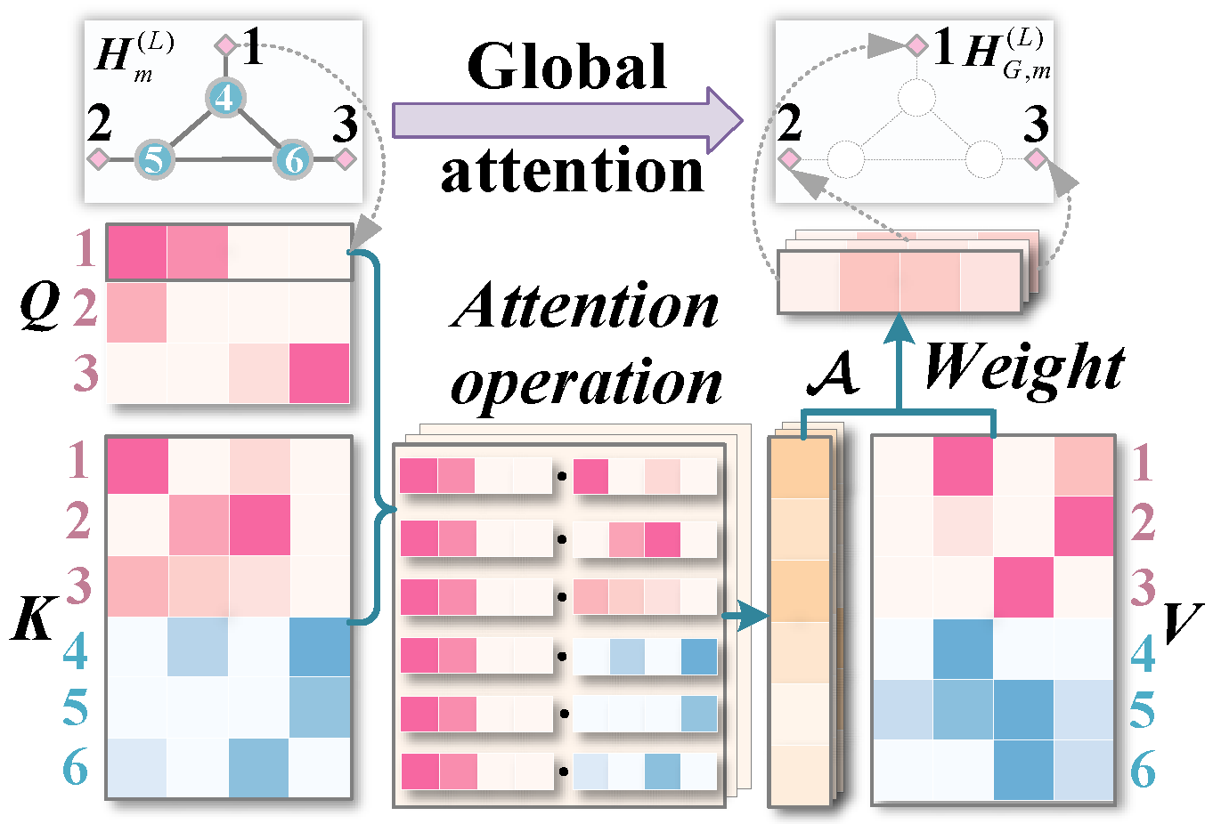
4.4. Global Attention Pooling

Transient stability is such a global problem that the stability results of each generator are related to the whole system. Given a representation matrix Z and its derivative versions in different spaces, including queries Q = Z W Q , keys K = Z W K and values V = Z W V , Transformer provides an effective global aggregation mode as [27]
T ( Q , K , V ) = softmax Q K T d k A V
where d k denotes the column dimension of W V while A refers to the matrix of global attention coefficients. Mathematically, (10) exploits the correlation between the feature matrix in the query and key space to weight that in the value space. The query space depends on the concerned target while the others rely on the relevant object of the target.
Our target is generators that are related to global (area) nodes. Assume H m ( L ) R R ( L ) × C ( L ) as the features of the m t h output coarsened graph with R ( L ) nodes. H m ( L ) is mapped to the key and value space but generator features H G , m ( L ) R N G × C ( L ) are only mapped to the query space. The global attention pooling is formulated as
H G , m P = T ( H G , m ( L ) W Q , m , H m ( L ) W K , m , H m ( L ) W V , m )
where W Q , m , W K , m and W V , m are parameter matrix of size C ( L ) × C ( L ) . Figure 7 exhibits physical generator-level operations in global attention pooling. The normalized dot product between a generator feature vector to be queried and keys at each node are acquired before a column-wise attention vector is acquired. It accounts for the significance of the interaction relationship between the generator and any other node. Then, the generator-level global representation is inherited from the weighted sum of all values based on the attention vector. Note that the transposed attention vectors form A m R N G × R ( L ) , which facilitates the scale reduction from areas to generators. The final generator representation matrix H G P = || m H G , m P is defined by concatenating H G , m P along rows.

4.5. Downstream Link

For the global representation of the i t h generator h G , i P , two downstream networks, DGP and GPP, predict dominant generators and generator severity, respectively.
DGP consists of a fully connected (FC) network f D G P ( · ) and a softmax function, which yields a confidence vector c ˜ i :
c ˜ i = softmax f D G P ( h G , i P )
where c ˜ i = [ c ˜ i 1 , c ˜ i 2 ] and c ˜ i 1 refers to the confidence that indicates whether a generator belongs to the dominant set.
GPP contains f G P P ( · ) and a softsign function [13] to provide predicted PSI-G η ˜ i
η ˜ i = softsign f G P P ( h G , i P )

5. Training and Evaluation of ECAP&GAP-GTSA Scheme

5.1. The Assistant Decision-Making of Generator

Given that DGP considers a generator dominantly unstable only if c ˜ i 1 0.5 ( S i 2 ) , while GPP considers a generator stable or unstable if η ˜ i > ε ( S i 3 ) or η ˜ i < ε ( S i 4 ) . The generator status is uncertain when η ˜ i ε , ε ( S i 5 ) . Overall, DGP has higher priority. The logic of ADM-G is listed as:
(1) The generator is included into G ˜ d once receiving S i 2 .
(2) Unless receiving S i 5 or ( S i 2 , S i 3 ), i.e., GPP considers the generator uncertain or GPP makes an opposite decision to that of DGP, η ˜ i is collected for η ˜ o .
(3) If receiving ( S i 2 , S i 4 ), both DGP and GPP provide unstable signals, while one of them provides an unstable signal when obtaining ( S i 2 , S i 3 ), ( S i 2 , S i 5 ) or ( S i 1 , S i 4 ). In such cases, the system is considered unstable ( c ˜ G 2 S = 0 ). Otherwise, the system is stable ( c ˜ G 2 S = 1 ).

5.2. Loss Function

The loss function L includes DGP loss L D G P , GPP loss L G P P and a sparsity-related loss L R = Θ 2 :
L = L D G P + L G P P + β 1 L R = b g ( L D G P , b g + L G P P , b g ) L G , b g / B G + β 1 L R
Θ contains the model parameters. The subscript “b”, “g” refer to the b t h sample and g t h generator, respectively. β 1 is set to 5 × 10 4 commonly. Based on a training set with total B G generators, L D G P , b g adopts the cross entropy function while L G P P , b g follows the smoothL1 function, similar to [11].

5.3. Definition of Evaluation Metrics

Performance metrics concerning DGP are proposed, including accuracy of dominant generator sets (ACC-DG), miss alarm of dominant generators (MA-DG) and coverage of dominant generator sets (Cov-DG). The first is acquired based on all the samples while the others aim at unstable ones.
Specifically, the Jaccard similarity is calculated between a predicted set and the labeled one as J ( G ˜ d , G d ) [22]. When J ( G ˜ d , G d ) = 1 , the set is perfectly predicted. ACC-DG focuses on the ratio of such cases:
ACC DG = n ( J ( G ˜ d , G d ) = 1 ) n ( J ( G ˜ d , G d ) = 1 ) B B
where n ( · ) denotes the number of cases. In terms of unstable scenarios with B G u dominant generators, MA-DG summarizes the classification errors of generators:
MA DG = 1 n ( c ˜ b i = c b i c b i = 0 ) n ( c ˜ b i = c b i c b i = 0 ) B G u B G u
With the accelerating unstable generator set G u , Cov-DG is a comprehensive metric to describe the reliability of predicted instability modes. Actually, the strict boundary might not exist in some critical cases where the dominant generators have similar short-term dynamics with the sub-dominant ones U G d G u . The control risk does not increase if a sub-dominant generator is assigned to the dominant set. Therefore, such a sample is considered reliable. For B u unstable samples, the Cov-DG is expressed as
Cov DG = n ( G d G ˜ d G u ) n ( G d G ˜ d G u ) B u B u
Assume B G the size of generators with definite PSI-G, mean square error of generators (MSE-G) is proposed for GPP
MSE G = b i η ˜ o , b i PSI G b i 2 b i η ˜ o , b i PSI - G b i 2 B G B G
The system-level prediction follows accuracy (ACC), miss alarm (MA) and false alarm (FA) in [13].

6. Case Studies

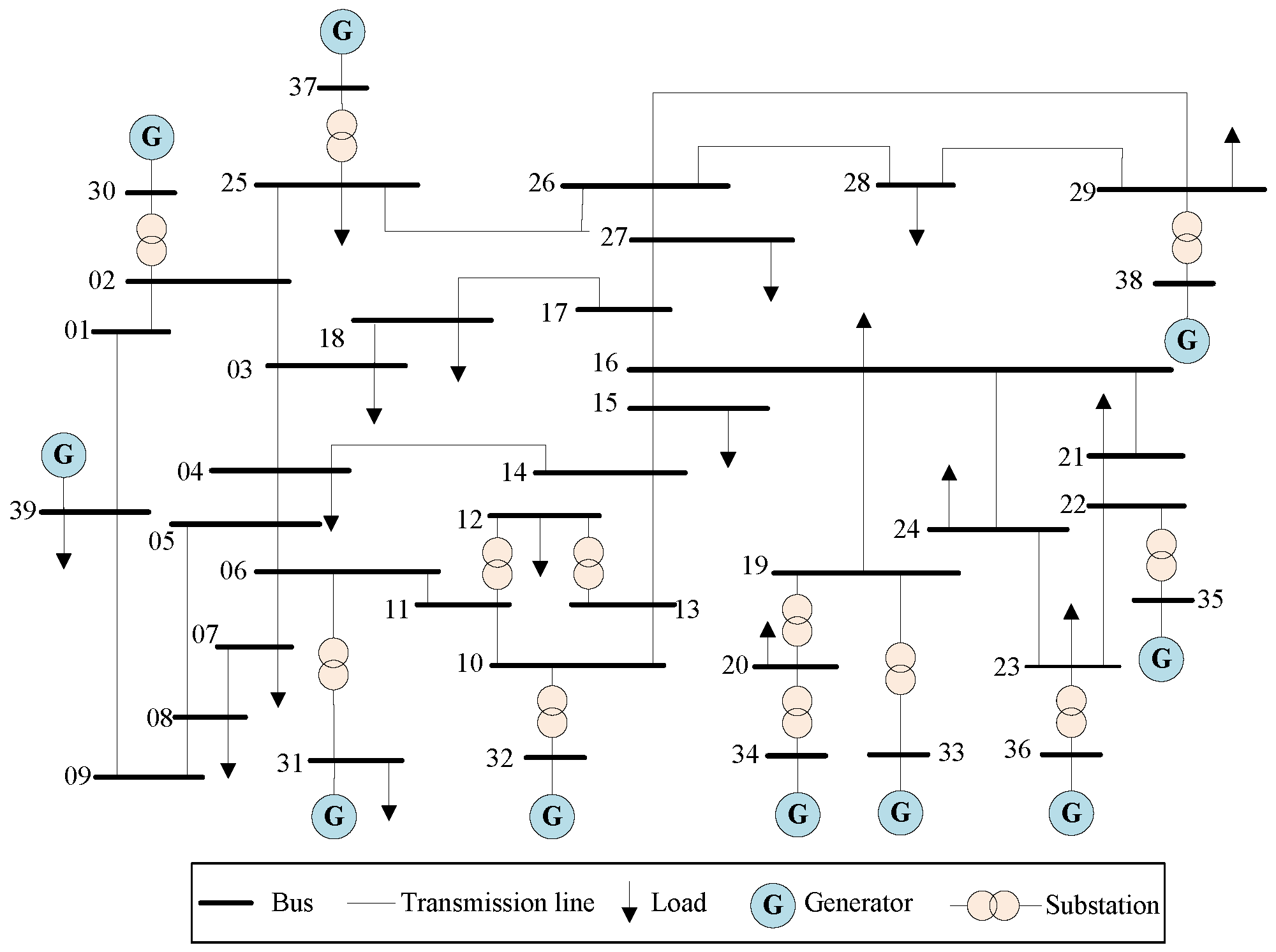
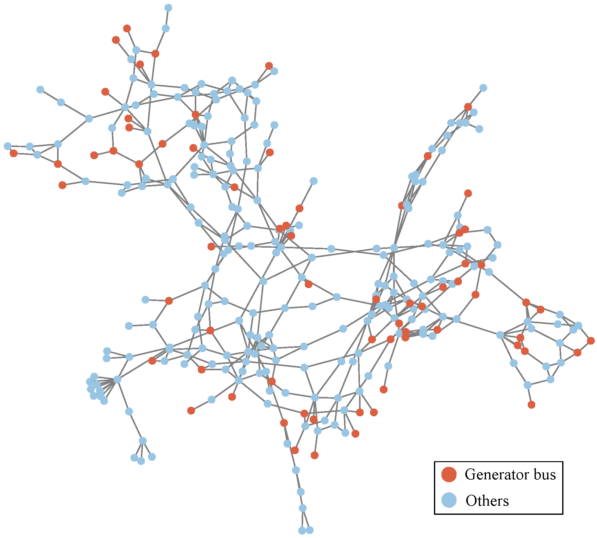
6.1. Test System and Model Setting

The ECAP&GAP-GTSA is verified on the IEEE 39-bus system first, as Figure 2. 46,319 samples are generated and divided into the training, validation and test set according to [13]. Note that the training set involves base operation conditions and “N-1” conditions, while the other two contain “N-2” conditions. There are parameters t t h = 0.1 s , ε = 0.1 and τ = 1.5 for label generation. Let R ( L ) be the scale of coarsened graphs after L ECAPs, which varies in different samples. The best model settings are listed in Table 1. N G , 39 and N G , 300 are the generator scales in different systems. Due to the limitation of computing device, the scale of parameters is 1.72 M and 1.16 M on the IEEE 39-bus system and IEEE 300-bus system. The averaging inference time of a sample on the two systems is 2.1 ms and 23 ms, which is merely 1/671 and 1/149 of that of TDS.

6.2. Comparisons with Existing GTSA Models

Existing GTSA models rely on dynamic inputs. Fairly, their structures are kept as baselines but substitute the steady-state information for the inputs. Note that RGCN is a spatio-temporal graph learning model. All the performance is illustrated in Table 2. Evidently, graph learning models demonstrate advance in all metrics. Ours beat the previous graph learning model with about 5% improvements in ACC and 6% in ACC-DG.

6.3. Pooling Methods and Structure Comparisons

To verify the advantage of sparse hybrid pooling, we replace it with global pooling [12] and dense pooling [13] as baselines, named GP and DP here. Test metrics are listed in Table 3. The GP neglects the inter-node difference and performs the worst. There are improvements in expressive DP , but it cannot generate areas with clear physical meaning and preserve network sparsity.
Furthermore, the decoupled structure in Figure 5 is also adopted for comparison, named →decoupled. It benefits from better generalization with sparse hybrid pooling, but lags significantly behind the proposed method in discriminating instability modes. The rationality of our pooling is well supported.

6.4. Detailed Advantage Analysis of Sparse Hybrid Pooling

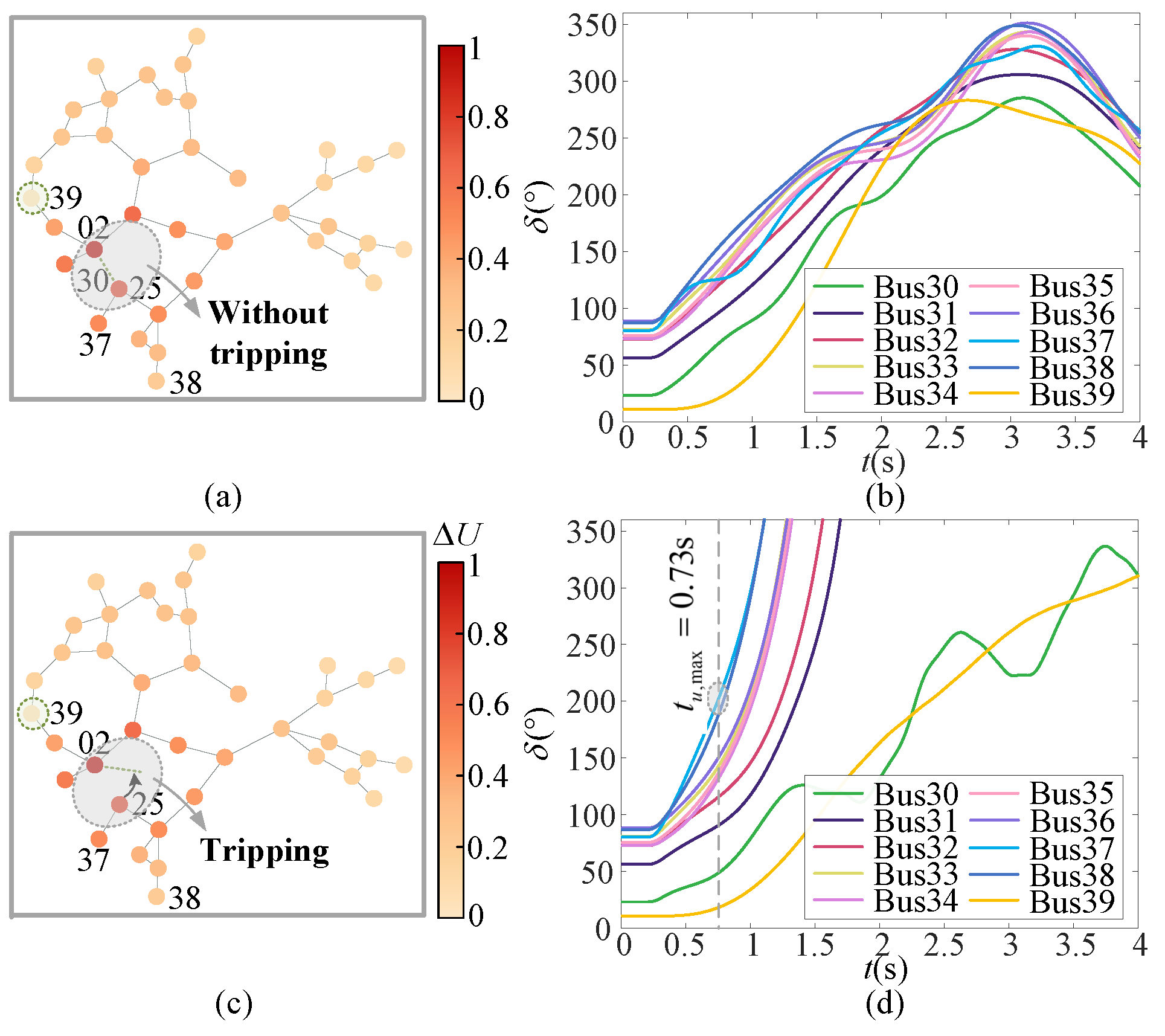
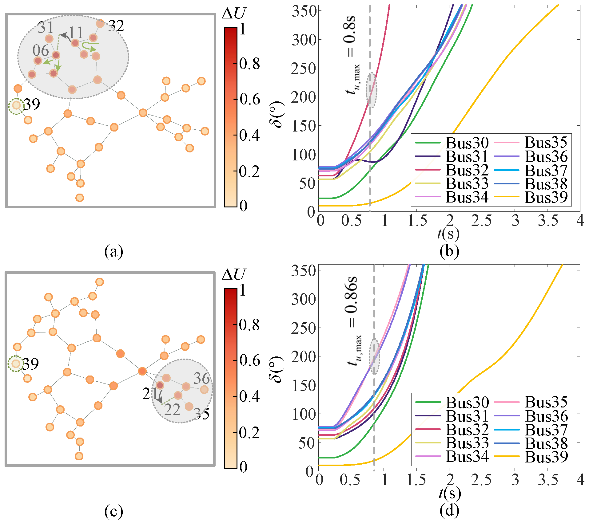
6.4.1. Ecap Visualization

In this section, the characteristics of ECAP are fully explained by visualizing the pooling of two cases.
The faulted line is bus 06-bus 11 in Case I-1 and bus 21-bus 22 in Case I-2. The TDS results are depicted in Figure 8. The visualizations are demonstrated in Figure 9 and Figure 10, where the mean voltage drops of (area) nodes are represented by color density and the generator nodes are highlighted.
Pay attention to the neighborhood (blue circle) of the faulted line bus 06-bus 11 in Case I-1. Two area nodes distinguished from the others are generated after node mergence. Inter-node relationships also become concise during network sparsification. From PSI-G prediction in Figure 11, the model discriminates the dominant generator connected to bus 32 in the faulted area owing to the reduction in the search range.
In terms of Case I-2, the transient impacts turn to the neighborhood of bus 35 and bus 36 when bus 21-bus 22 are faulted. These buses keep strong connections during the pooling such that the model assigns them as dominant generators, which is consistent with TDS results. Compared with Case I-1, the pooling strategy concerning bus 31 and bus 32 changes, i.e., they are connected to the same area. Thus, they are correctly predicted coherent and stable.
Case II is the same one as discussed in Figure 1 with the faulted line bus 02-bus 25. The key areas lie in the neighborhood of bus 30 and bus 37. After annotating the inter-case differences with stars, it is interesting that the aggregation modes are almost the same in areas far away from the key ones. Such robustness encourages the model to focus on the slight topology difference. In Case II-1, bus 37 and bus 38 deliver powers through various lines during pooling and contribute to the final ring-like structure, as Figure 12d. On the contrary, line tripping leads to difficulty in power delivery and chain-like structure in Case II-2, as Figure 13d. Then, our model quantifies the generator-level stability contrast and yields accurate indexes in Figure 14.

6.4.2. Gap Visualization

The relationships between attention matrix A m of GAP and coarsened topologies and generator dynamics and labels are explored here. A m is described by a heatmap in Figure 15b. Here, the vertical axis refers to the number of generator buses, while the horizontal axis denotes the number of different node representations in final pooled graphs (e.g., No.1, No.16 and No.31 represent the features at the first node in G 1 ( L ) , G 2 ( L ) and G 3 ( L ) ) after graph embedding.
In Figure 15b, bus 37 and bus 38 exhibit distinct characteristics in the heatmap. They are not only related to their own representations but also strongly concerned with the remote one highlighted by a green dotted circle in Figure 15a. Such global and reasonable attention distribution facilitates model performance. As Figure 15d, it assigns bus 37 and bus 38 to the dominant generator set and identifies generator groups, which accord with the real dynamics in Figure 15c.

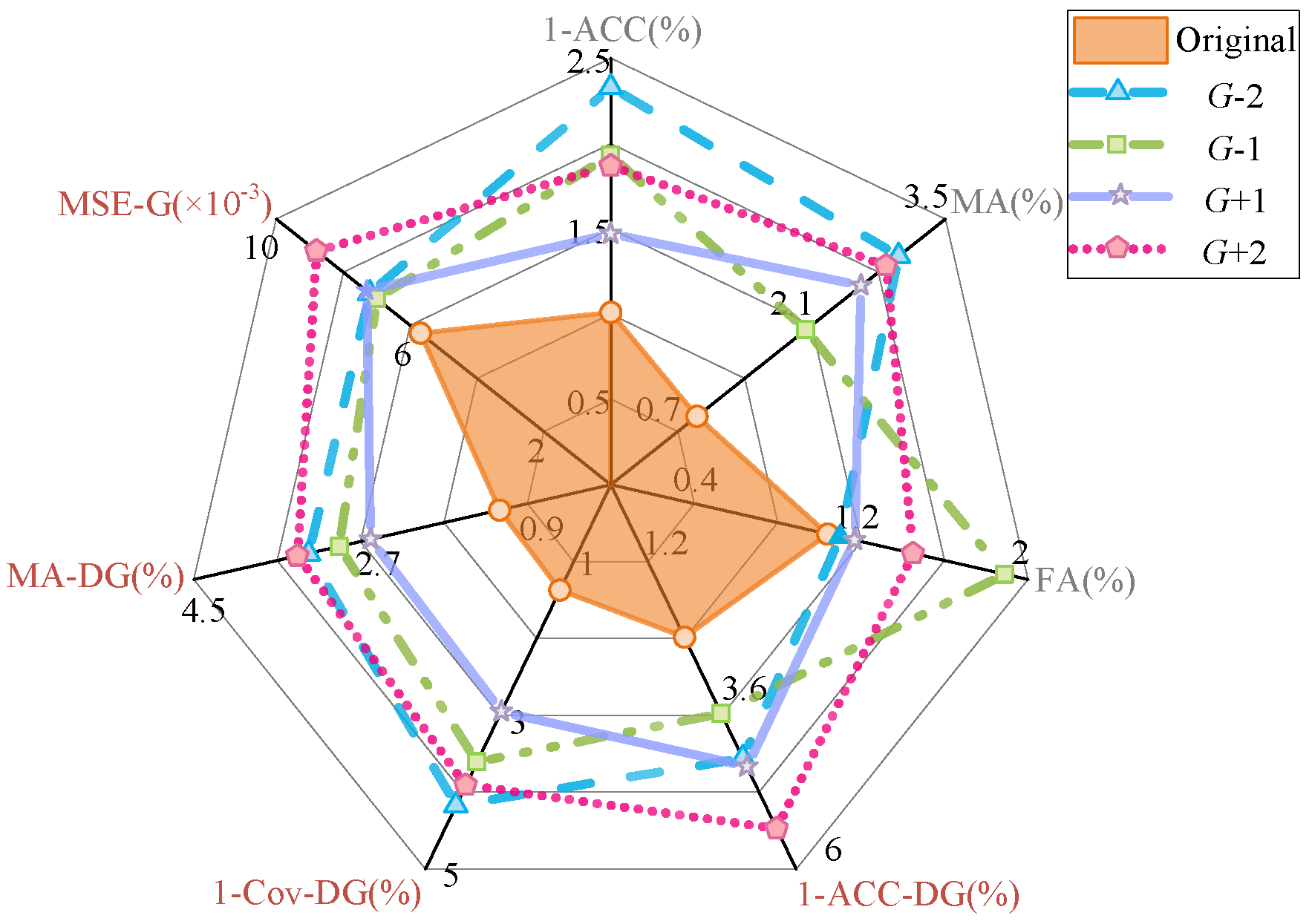
6.5. Robustness and Scalability to Generator-Scale Changes

6.5.1. Modified IEEE 39-Bus Systems

First, four systems with different generators called “ G ± K ” are derived from the IEEE 39-bus system, where K denotes the varied generator scale [13]. Each corresponds to 3000 samples. In such a context, existing GTSA fails, but our ECAP&GAP-GTSA provides high-quality results without retraining. The performance metrics are depicted in Figure 16. Assume the original scenario refers to the test set. The generator-level and system-level metrics are emphasized with red and gray font. It is noticed that ACC is always over 97.5%, while ACC-DG keeps above 94.5%. In terms of the instability mode prediction, MA-DG is less than 4% and the output generator sets cover dominant generators correctly in more than 96% samples. This proves our robustness against various generator-scale changes.

6.5.2. IEEE 300-Bus System

On the IEEE 300-bus system with 69 generators in Figure 17, 52,210 samples are generated including 38,160 stable ones and 14,050 unstable ones. Based on the best model settings in Table 1, our generalization is verified in Table 4. There is little performance loss though the generator scale rises significantly, which accounts for our superiority in scalability.

7. Conclusions

In this paper, an ECAP&GAP-GTSA scheme is proposed to provide dominant generators and generator severity after perturbation for preventive controls. It is complementary to GTSA schemes based on steady-state information. First, the generalization and interpretability are both guaranteed via sparse hybrid pooling. ECAP achieves scale reduction by edge contraction and ensures the inter-node difference as well as network sparsity. GAP assigns a representative vector for each generator such that the scale of pooled representations is consistent with that of generators. On the other hand, the combination of GAP and generator-sharing downstream networks enables the model to work under generator-scale changes. Test results on the IEEE 39-bus system and IEEE 300-bus system demonstrate the outstanding performance of ECAP&GAP-GTSA in scenarios with various operation topologies. Under slight generator-scale changes during long-term operation, the model accuracy is at least 94.5% without retraining. When applied to the larger system with retraining, the accuracy reaches about 99% with an inference time of merely 23 ms. This indicates that the model meets both the reliability and real-time requirements of real-world operation.

8. Discussion

In real-world power systems, system-level and generator-level indexes are both necessary. The former provides early warning and the latter benefits the preventive control scheme. Though the generator-level indexes and a discrete system-level index, i.e., system status, are available here, the continuous system-level index to represent the stability trend is still missing. It means the operators cannot be aware of the risk level intuitively. Hence, our future works will focus on the integration of system-level and generator-level models in real-world systems. The sparse pooling method is also expected to promote the system-level model performance. Furthermore, we will pay attention to the assessment model on system-level frequency and voltage stability.

Author Contributions

Conceptualization, J.H. and L.G.; Data curation, Z.C.; Funding acquisition, L.G.; Methodology, J.H. and L.G.; Project administration, Y.S.; Software, L.C. and Y.L.; Supervision, J.H. and L.G.; Validation, J.Z.; Writing—original draft, J.H. and L.G.; Writing—review & editing, J.H. and L.G. All authors have read and agreed to the published version of the manuscript.

Funding

This work is supported by China Southern Power Grid Research under Project (ZBKJXM20240193).

Data Availability Statement

The data will be available on request.

Conflicts of Interest

Author Jiyu Huang was employed by the company CSG Energy Development Research Institute Co., Ltd.; Author Liukai Chen was employed by the company CSG Electric Power Research Institute Co., Ltd. The remaining authors declare that the research was conducted in the absence of any commercial or financial relationships that could be construed as a potential conflict of interest.

Nomenclature

TDSTime-domain simulation
TSATransient stability assessment
MLMachine learning
GTSAGenerator-level transient stability assessment
SVMSupport vector machine
ANNArtificial neural network
RFRandom forest
DLDeep learning
CNNConvolutional neural network
LSTMLong short-term menmory
ViTVision Transformer
RGCNRecurrent graph convolutional network
ECAPEdge Contraction-based Attention Pooling
GAPGlobal Attention Pooling
DGPDominant generator predictor
GPPGenerator perturbation predictor
ADM-GAssistant decision-making of generator
ACC-DGAccuracy of dominant generator sets
MA-DGmiss alarm of dominant generators
Cov-DGAccuracy of dominant generator sets
PSI G i The piece transient stability index of the i t h generator
N, N G The number of buses, the number of those connected with generator in a power system
x 0 , y 0 The state variables, algebraic variables
G ¯ m Parameterized topologies
G m ( 0 ) , V m ( 0 ) Input graphs and nodes
X m , A m Input node feature matrix, adjacency matrix
δ i ( t ) The angle of the i t h generator at the moment t
| Δ δ ( t ) | The maximum angle difference among any two generator at the moment t
Δ δ r , i , max The maximum relative angle difference
t u , m a x The first time | Δ δ ( t ) | exceeds 180
G , G d , G u The generator set, dominant generator set, unstable generator set
N d , t t h The number threshold of generator, time window of the affinity propagation (AP) cluster
ρ , ρ ( i , i ) The similarity matrix, its element of the affinity propagation (AP) cluster
G p The generator pair at the moment t that accounts for | Δ δ ( t ) |
c i The dominant status of the i t h generator
θ r e f ( t ) The TDS curves of the voltage phase of the chosen reference bus
t u , i , t u , i The instablity time and its normalized version of the i t h generator
C δ , max A constant that represents the maximum of all Δ δ r , i , max in the history data
μ u , ξ u The mean, variance of all t u , i in the history data
τ The modulation factor of PSI-G
σ ( · ) The sigmoid function
σ leaky The LeakyReLu function
ε The parameter to form an uncertain area
H m ( l ) , h m i ( l ) The output matrix, its i t h row vector of the m t h graph in the l t h graph convolution (“Conv”) layer
R ( l ) , C ( l ) The (coarsened) system scale and feature dimension in the l t h graph pooling (“Pool”) layer
R ( l ) , C ( l ) The (coarsened) system scale and feature dimension in the l t h ECAP layer
V q c ( l + 1 ) , V q ( l + 1 ) The q t h node sets of the old graph to be merged in the l t h ECAP layer, the  q t h node of the new graph in the ( l + 1 ) t h ECAP layer
K e The number of attention heads of ECAP layers
W e , k ( l ) The parameter matrix of the k t h attention head
α e , k ( i , j ) ( l ) The attention coefficient from node j to node i of the k t h head in the l t h ECAP layer
s ( i , j ) ( l ) The edge score from node V j ( l ) to node V i ( l )
N m , i ( l ) The 1st-order neighborhood set of the i t h node in the m t h graph
W c The transformation matrix for the data-driven features
H m ( L ) , H G , m ( L ) The features of all the nodes, the generator nodes in the m t h output coarsened graph
W Q , m , W K , m , W V , m The parameter matrics to generate keys, queries and values
A m The attention matrix of the m t h graph in the GAP
H G P , h G , i P The final representation(s) of all the generators, the  i t h generator
f D G P ( · ) , f G P P ( · ) The function of DSP, GPP
c ˜ i 1 , η ˜ i The confidence level of c i = 0 , the prediction of PSI - G i
S i 1 S i 5 The logical signals derived from the model prediction
G ˜ d , η ˜ o , c ˜ G 2 S The prediction of dominant generator, generator severity vector, system-level stability category after the ADM-G
L , L D G P , L G P P , L R The loss functions concerning the whole model, DGP, GPP, sparsity

References

  1. Obuz, S.; Ayar, M.; Trevizan, R.D.; Ruben, C.; Bretas, A.S. Renewable and energy storage resources for enhancing transient stability margins: A PDE-based nonlinear control strategy. Int. J. Elec. Power 2020, 116, 105510. [Google Scholar] [CrossRef]
  2. Yu, J.J.Q.; Hill, D.J.; Lam, A.Y.S.; Gu, J.; Li, V.O.K. Intelligent Time-Adaptive Transient Stability Assessment System. IEEE Trans. Power Syst. 2016, 33, 1049–1058. [Google Scholar] [CrossRef]
  3. Yan, R.; Geng, G.; Jiang, Q.; Li, Y. Fast transient stability batch assessment using cascaded convolutional neural networks. IEEE Trans. Power Syst. 2019, 34, 2802–2813. [Google Scholar] [CrossRef]
  4. Shi, Z.; Yao, W.; Zeng, L.; Wen, J.; Fang, J.; Ai, X.; Wen, J. Convolutional neural network-based power system transient stability assessment and instability mode prediction. Appl. Energy 2020, 263, 114586. [Google Scholar] [CrossRef]
  5. Lotufo, A.D.P.; Lopes, M.L.M.; Minussi, C.R. Sensitivity analysis by neural networks applied to power systems transient stability. Electr. Power Syst. Res. 2007, 77, 730–738. [Google Scholar] [CrossRef]
  6. Zhou, Y.; Wu, J.; Ji, L.; Yu, Z.; Lin, K.; Hao, L. Transient stability preventive control of power systems using chaotic particle swarm optimization combined with two-stage support vector machine. Electr. Power Syst. Res. 2018, 155, 111–120. [Google Scholar] [CrossRef]
  7. Liu, X.; Min, Y.; Chen, L.; Zhang, X.; Feng, C. Data-driven transient stability assessment based on kernel regression and distance metric learning. J. Mod. Power Syst. Cle. 2020, 9, 27–36. [Google Scholar] [CrossRef]
  8. Liu, Y.; Zhai, M.; Jin, J.; Song, A.; Zhao, Y. Intelligent Online Catastrophe Assessment and Preventive Control via a Stacked Denoising Autoencoder. Neurocomputing 2019, 380, 306–320. [Google Scholar] [CrossRef]
  9. Ren, J.; Chen, J.; Shi, D.; Li, Y.; Li, D.; Wang, Y.; Cai, D. Online multi-fault power system dynamic security assessment driven by hybrid information of anticipated faults and pre-fault power flow. Int. J. Electr. Power 2022, 136, 107651. [Google Scholar] [CrossRef]
  10. Wang, K.; Wei, W.; Xiao, T.; Huang, S.; Zhou, B.; Diao, H. Power system preventive control aided by a graph neural network-based transient security assessment surrogate. Energy Rep. 2022, 8, 943–951. [Google Scholar] [CrossRef]
  11. Huang, J.; Guan, L.; Su, Y.; Yao, H.; Guo, M.; Zhong, Z. A topology adaptive high-speed transient stability assessment scheme based on multi-graph attention network with residual structure. Int. J. Elec. Power 2021, 130, 106948. [Google Scholar] [CrossRef]
  12. Huang, J.; Guan, L.; Su, Y.; Yao, H.; Guo, M.; Zhong, Z. System-Scale-Free Transient Contingency Screening Scheme Based on Steady-State Information: A Pooling-Ensemble Multi-Graph Learning Approach. IEEE Trans. Power Syst. 2021, 37, 294–305. [Google Scholar] [CrossRef]
  13. Huang, J.; Guan, L.; Chen, Y.; Zhu, S.; Chen, L.; Yu, J. A deep learning scheme for transient stability assessment in power system with a hierarchical dynamic graph pooling method. Int. J. Electr. Power 2022, 141, 108044. [Google Scholar] [CrossRef]
  14. Guo, T.; Milanović, J.V. Online identification of power system dynamic signature using PMU measurements and data mining. IEEE Trans. Power Syst. 2015, 31, 1760–1768. [Google Scholar] [CrossRef]
  15. Frimpong, E.; Asumadu, J.; Okyere, P. Real time prediction of coherent generator groups. J. Electr. Eng. 2016, 16, 47–56. [Google Scholar]
  16. Siddiqui, S.A.; Verma, K.; Niazi, K.; Fozdar, M. Real-time monitoring of post-fault scenario for determining generator coherency and transient stability through ANN. IEEE Trans. Ind. Appl. 2017, 54, 685–692. [Google Scholar] [CrossRef]
  17. Mazhari, S.M.; Safari, N.; Chung, C.; Kamwa, I. A quantile regression-based approach for online probabilistic prediction of unstable groups of coherent generators in power systems. IEEE Trans. Power Syst. 2018, 34, 2240–2250. [Google Scholar] [CrossRef]
  18. Pavlatos, C.; Makris, E.; Fotis, G.; Vita, V.; Mladenov, V. Enhancing Electrical Load Prediction Using a Bidirectional LSTM Neural Network. Electronics 2023, 12, 4652. [Google Scholar] [CrossRef]
  19. Gupta, A.; Gurrala, G.; Sastry, P.S. An Online Power System Stability Monitoring System Using Convolutional Neural Networks. IEEE Trans. Power Syst. 2019, 34, 864–872. [Google Scholar] [CrossRef]
  20. Fang, J.; Liu, C.; Zheng, L.; Su, C. A data-driven method for online transient stability monitoring with vision-transformer networks. Int. J. Electr. Power 2023, 149, 109020. [Google Scholar] [CrossRef]
  21. Zhu, L.; Wen, W.; Li, J.; Hu, Y. Integrated Data-Driven Power System Transient Stability Monitoring and Enhancement. IEEE Trans. Power Syst. 2023, 39, 1797–1809. [Google Scholar] [CrossRef]
  22. Huang, J.; Guan, L.; Su, Y.; Yao, H.; Guo, M.; Zhong, Z. Recurrent Graph Convolutional Network-Based Multi-Task Transient Stability Assessment Framework in Power System. IEEE Access 2020, 8, 93283–93296. [Google Scholar] [CrossRef]
  23. Diehl, F.; Brunner, T.; Le, M.T.; Knoll, A. Towards graph pooling by edge contraction. In Proceedings of the 36th International Conference on Machine Learning, Long Beach, CA, USA, 9–15 June 2019. [Google Scholar]
  24. Xue, Y.; Van Custem, T.; Ribbens-Pavella, M. Extended equal area criterion justifications, generalizations, applications. IEEE Trans. Power Syst. 1989, 4, 44–52. [Google Scholar] [CrossRef]
  25. Frey, B.J.; Dueck, D. Clustering by passing messages between data points. Science 2007, 315, 972–976. [Google Scholar] [CrossRef]
  26. Baek, J.; Kang, M.; Hwang, S.J. Accurate Learning of Graph Representations with Graph Multiset Pooling. In Proceedings of the 8th International Conference on Learning Representations (ICLR 2020), Addis Ababa, Ethiopia, 26–30 April 2020. [Google Scholar]
  27. Vaswani, A.; Shazeer, N.; Parmar, N.; Uszkoreit, J.; Jones, L.; Gomez, A.N.; Kaiser, L.; Polosukhin, I. Attention is All You Need. In Proceedings of the 31st Conference on Neural Information Processing Systems (NIPS 2017), Long Beach, CA, USA, 4–9 December 2017. [Google Scholar]
Figure 1. Transient cases under different clearing modes. (a,c) The transient impacts in two cases. (b,d) The angle curves.
Electronics 14 01180 g001
Figure 2. One-line diagram of the IEEE 39-bus system.
Electronics 14 01180 g002
Figure 3. Comparison on the ECAP&GAP-GTSA and an existing scheme [9].
Electronics 14 01180 g003
Figure 4. ECAP&GAP-GTSA scheme.
Electronics 14 01180 g004
Figure 5. Pooling-convolution structures. (a) decoupled. (b) coupled.
Electronics 14 01180 g005
Figure 6. The rule of ECAP.
Electronics 14 01180 g006
Figure 7. The rule of global attention pooling.
Electronics 14 01180 g007
Figure 8. Transient cases under different fault locations. (a,c) Transient impacts in Case I-1 and I-2. (b,d) Their angle curves.
Electronics 14 01180 g008
Figure 9. Pooling of Case I-1 in the (a) 1st, (b) 2nd, (c) 3rd and (d) 4th ECAP layer.
Electronics 14 01180 g009
Figure 10. Pooling of Case I-2 in the (a) 1st, (b) 2nd, (c) 3rd and (d) 4th ECAP layer.
Electronics 14 01180 g010
Figure 11. PSI-G prediction. (a) Case I-1. (b) Case I-2.
Electronics 14 01180 g011
Figure 12. Pooling of Case II-1 in the (a) 1st, (b) 2nd, (c) 3rd and (d) 4th ECAP layer.
Electronics 14 01180 g012
Figure 13. Pooling of Case II-2 in the (a) 1st, (b) 2nd, (c) 3rd and (d) 4th ECAP layer.
Electronics 14 01180 g013
Figure 14. PSI-G prediction. (a) Case II-1. (b) Case II-2.
Electronics 14 01180 g014
Figure 15. Global attention pooling visualization. (a) Coarsened topology. (b) Attention matrix. (c) Generator dynamics. (d) PSI-G predictions.
Electronics 14 01180 g015
Figure 16. Performance metrics under generator-scale changes.
Electronics 14 01180 g016
Figure 17. Graphical IEEE 300-bus system.
Electronics 14 01180 g017
Table 1. Best model settings.
LayerIEEE 39-Bus SystemIEEE 300-Bus System
DGPGPPDGPGPP
Graph embedding (input size, output size, head(s))
conv1(3 × 39 × 5, 3 × 39 × 16, 6)(3 × 300 × 5, 3 × 300 × 16, 6)
ecap1(3 × 39 × 96, 3 × R ( 1 ) × 96, 6)(3 × 300 × 96, 3 × R ( 1 ) × 101, 6)
conv2(3 × R ( 1 ) × 101, 3 × R ( 1 ) × 24, 6)(3 × R ( 1 ) × 101, 3 × R ( 1 ) × 16, 6)
ecap 2(3 × R ( 1 ) × 144, 3 × R ( 2 ) × 149, 6)(3 × R ( 1 ) × 96, 3 × R ( 2 ) × 101, 6)
conv3(3 × R ( 2 ) × 149, 3 × R ( 2 ) × 32, 6)(3 × R ( 2 ) × 101, 3 × R ( 2 ) × 24, 6)
ecap3(3 × R ( 2 ) × 192, 3 × R ( 3 ) × 197, 6)(3 × R ( 2 ) × 144, 3 × R ( 3 ) × 149, 6)
conv4(3 × R ( 3 ) × 192, 3 × R ( 3 ) × 48, 6)(3 × R ( 3 ) × 49, 3 × R ( 3 ) × 24, 6)
ecap 4-(3 × R ( 3 ) × 144, 3 × R ( 4 ) × 149, 6)
conv5-(3 × R ( 4 ) × 149, 3 × R ( 4 ) × 32, 6)
Global attention pooling (input size, output size)
gap(3 × R ( 3 ) × 192, N G , 39 × 864)(3 × R ( 4 ) × 149, N G , 300 × 576)
Downstream network (input size, output size)
fc1(864,128)(864,128)(576,128)(576,128)
fc2(128,16)(128,16)(128,16)(128,16)
fc3(16,2)(16,1)(16,2)(16,1)
Remark: “conv”, “ecap” and “gap” denote convolution, ECAP and global attention pooling.
Table 2. Performance compared with GTSA baselines.
System-LevelGenerator-Level
ModelACCMAFAACC-DGCov-DGMA-DGMSE-G
(%)↑(%)↓(%)↓(%)↑(%)↑(%)↓( × 10 3 )↓
SVM [14]92.2118.655.4088.3865.0932.6818.4
RF [17]92.1225.284.0489.2558.8847.6319.7
ANN [16]92.6721.824.1489.4364.0834.1815.3
CNN [19]91.0212.318.2588.0973.1017.9122.6
RGCN [22]94.117.355.5791.9984.7014.3112.9
Proposed98.990.901.0497.6298.631.205.7
Remark: ↑, means the larger the better. ↓ does the opposite. Bold values refer to the best performance.
Table 3. Performance compared with pooling baselines.
System-LevelGenerator-Level
ModelACCMAFAACC-DGCov-DGMA-DGMSE-G
(%)↑(%)↓(%)↓(%)↑(%)↑(%)↓( × 10 3 )↓
GP 97.345.801.9695.5183.3811.8911.9
DP 98.373.051.3296.5391.876.916.7
→decoupled98.503.231.1296.9193.195.636.3
Proposed98.990.901.0497.6298.631.205.7
Table 4. Performance on the IEEE 300-bus system.
System-LevelGenerator-Level
ACCMAFAACC-DGCov-DGMA-DGMSE-G
(%)↑(%)↓(%)↓(%)↑(%)↑(%)↓( × 10 3 )↓
98.961.390.9597.4897.392.397.8
Disclaimer/Publisher’s Note: The statements, opinions and data contained in all publications are solely those of the individual author(s) and contributor(s) and not of MDPI and/or the editor(s). MDPI and/or the editor(s) disclaim responsibility for any injury to people or property resulting from any ideas, methods, instructions or products referred to in the content.

