Prediction of Dissolved Gases in Transformer Oil Based on CEEMDAN-PWOA-VMD and BiGRU

Abstract

Aiming at improving the prediction accuracy of the gas dissolved in transformer oil which occurs with strong nonlinearity, this paper presents a method named CEEMDAN-PWOA-VMD-BIGRU for gas content prediction. First, Complete Ensemble Empirical Mode Decomposition with Adaptive Noise (CEEMDAN) is performed to decompose the original gas sequence. To solve the problem of the strong nonlinear characteristic of the decomposed high-frequency components leads to a large error in prediction, this paper uses Variational Mode Decomposition (VMD) for secondary decomposition. Though VMD can decompose high-frequency modes well, the selection of the optimal decomposition number and the quadratic penalty factors often depends on subjective judgment, which may affect the accuracy of decomposition results. Therefore, Whale Optimization Algorithm (WOA) is applied to optimize the parameter setting of VMD. However, the search of WOA in the optimization process is random, which leads to the limitations of the optimization efficiency. To solve this problem, this paper further uses Proximal Policy Optimization (PPO) to improve WOA (PWOA). With the optimized parameters of PWOA, VMD obtains more accurate secondary decomposition results. Then, the trained Bidirectional Gated Recurrent Unit (BiGRU) model is used to predict each decomposed component, and finally these predicted components are reconstructed to obtain more accurate prediction results. The experimental results demonstrate that the mean absolute error (MAE) of the proposed model is reduced by 6.88%, 7.45%, and 5.69%, compared with the traditional algorithms of Long Short-term Memory network (LSTM), Gated Recurrent Unit (GRU), and Temporal Convolution Network (TCN), respectively.

1. Introduction

The oil-immersed transformer is one of the critical equipment in a grid, which directly influences the safe and stable operation of the whole system. It is essential to monitor the operating status of transformers and warn latent faults in advance [1]. Dissolved Gas Analysis (DGA) is currently a useful means for the diagnosis of the potential faults in transformers and has been widely applied [2]. The prediction of the variation tendency of the gas dissolved in the oil plays a crucial role in the early warning of the transformer failures [3]. The generation of dissolved gases is closely related to internal faults of the transformer, so the time series of the gases dissolved in the oil exhibit high complex and nonlinear characteristics, which seriously affect the prediction accuracy [4,5]. Meanwhile, DGA is the basis for evaluating the insulation condition of power transformers. By detecting and quantifying the concentrations of key gases (such as H₂, CH₄, C₂H₄, CO, etc.), DGA can reveal smaller faults, such as partial discharges, thermal degradation, and arcs. The diagnostic accuracy of DGA not only depends on advanced algorithms, but fundamentally on the quality and interpretability of gas data, which reflects the physical and chemical interactions within the insulation system. Therefore, effective DGA data is equally crucial for preventing catastrophic failures and optimizing maintenance strategies.

In recent years, significant research has been devoted to the prediction of the dissolved gas content in transformer oil. Some scholars focus their studies on classical time series analysis theories such as the gray prediction theory [6] or time series models [7]. The established regression model is relatively simple, and it is difficult to reflect the characteristics of the gas content changes in transformer oil, which are highly nonlinear, non-stationary, and random. Therefore, some scholars adopt machine learning methods for gas content prediction. In the literature [8], SVM is used to predict the gas content, which defines the objective function in the feature space based on the structural risk minimization. In contrast, AI forecasting methods have been continuously developed, which are gradually becoming the mainstream approach for time series prediction. Traditional AI algorithms include Support Vector Regression (SVR) [9], Multi-Layer Perceptron (MLP) models, etc. However, these methods have gradually been replaced by Recurrent Neural Network (RNN) models [10], which are superior at capturing the relationships and dependencies between time series data. LSTM is commonly used variant of RNN which addresses the “vanishing gradient” and “exploding gradient” problems inherent in standard RNNs [11]. However, considering that the training time of LSTM is quite long, another variant of RNN called GRU has emerged. The GRU has a simpler gating mechanism than LSTM, fewer parameters, and faster training speed, and is more efficient in handling long time series data. The BiGRU, which is built upon the GRU, utilizes both historical and prospective information for prediction, which enhances the prediction accuracy [12].

The significant advancements of decomposition techniques in fields of forecasting have been widely concerned by researchers in recent years. For nonlinear and non-stationary time series, reference [13] employed wavelet decomposition (WD) to handle the non-stationarity of gas series. However, this approach is sensitive to the selection of the basis function and lacks adaptability. References [14,15] introduced Empirical Mode Decomposition (EMD) to stabilize non-stationary and nonlinear time sequences, which overcomes the challenges associated with the wavelet basis selection and the decomposition scales of the wavelet decomposition. Reference [16] utilized Ensemble Empirical Mode Decomposition (EEMD), which mitigates the mode aliasing issue inherent in EMD. Reference [17] proposed Complete Ensemble Empirical Mode Decomposition (CEEMD), which effectively resolves the mode mixing problem and eliminates the reconstruction errors that may arise in EEMD. In reference [18], CEEMDAN was improved by introducing adaptive noise, which further enhances the precision and the robustness of the signal decomposition.

However, due to the high-frequency modes in CEEMDAN, decomposition often contains noise, sudden events, and strong nonlinearity; the prediction errors through directly forecasting by these modes are relatively large. In reference [19], the authors employed an improved Complementary Ensemble Empirical Mode Decomposition (ICEEMDAN) based on adaptive noise and a secondary decomposition of an improved VMD algorithm. This approach resulted in better forecasting, compared to both single decomposition and direct prediction methods. In reference [20], a prediction model was developed using EMD-VMD secondary modal decomposition and GA-BP. By employing the VMD to decompose the high-frequency modal components, the prediction accuracy of the carbon price was notably enhanced. However, in related studies, the key parameters of the VMD algorithm were not optimized but only chosen subjectively, which lead to uncertainty and instability, which potentially cause excessive reconstruction errors, thereby restraining the prediction accuracy. To address this issue, references [21,22], respectively, employed the Hiking Optimization Algorithm (HOA) and Artificial Hummingbird Algorithm (AHA) to optimize the key parameters of VMD. However, these algorithms are relatively poor at global optimization and are prone to getting stuck in local optima. The WOA simulates the behavior of the whale groups, which enables more effective exploration in the entire solution space, and it is characterized by strong global search capabilities [23]. However, the search process in the WOA exhibits stochastic behavior, which may result in fluctuations and uncertainty in the optimization [24]. To enhance the stability and effectiveness of the optimization, it is necessary to address the stochastic property of the search process in WOA. Reinforcement learning (RL), an improved AI technique, has been successfully utilized in industrial control in recent years. RL learns the best decision-making strategies through interactions between the agent and the environment to maximize the rewards. However, RL faces significant limitations in high-dimensional problems [25]. To overcome these challenges, deep reinforcement learning (DRL) integrates the deep perception and decision-making capacity of deep learning. By extracting the latent information through DRL, the effectiveness of the WOA can be effectively enhanced, thus addressing the instability issues in its search process. In this context, the Proximal Policy Optimization (PPO) algorithm, with its rapid convergence speed and high sample efficiency, has attracted significant attention in DRL problems [26]. This paper introduces the PPO algorithm to further improve WOA, which effectively enhances the stability and the convergence speed, thereby manifesting significant superiority in handling complex optimization problems.

In summary, this paper proposes a prediction model of gas dissolved in transformer oil based on CEEMDAN-PWOA-VMD-BiGRU. The main innovations can be summarized as follows:

• In response to the high volatility and nonlinearity of the dissolved gases in transformer oil, a secondary decomposition approach is proposed. Specifically, the CEEMDAN decomposition method is applied for primary decomposition, then VMD secondary decomposition is utilized for the higher-complexity modal components.
• Since the key parameters of the VMD algorithm used in the secondary decomposition are dependent on subjective settings, it may lead to excessive reconstruction errors and a subsequent decrease in prediction accuracy. To address this issue, this paper proposes an improved WOA, which possesses strong global search capabilities, achieves optimized selection for the critical parameters of the VMD algorithm, and ensures the effectiveness of modal decomposition.
• Considering that WOA exhibits randomness in searching during the optimization process, which leads to fluctuations and uncertainties in the optimization, this study integrates WOA and the PPO algorithm, thereby effectively resolving the instability issues and enhancing the solution efficiency.

The structure of the remainder of this article is as follows: Section 2 and Section 3 present primary decomposition based on CEEMDAN and secondary decomposition using PWOA-VMD, respectively. Section 4 and Section 5 describe the BiGRU prediction model and the prediction model of gas dissolved in transformer oil based on CEEMDAN-PWOA-VMD-BiGRU, respectively. Finally, Section 6 provides an analysis of the experimental results, and Section 7 presents the conclusions derived from the paper.

2. Primary Decomposition Based on CEEMDAN

EMD is an adaptive method widely used for analyzing nonlinear and non-stationary signals. To tackle mode mixing in EMD, researchers introduced EEMD and CEEMDAN. EEMD prevents mode mixing by adding white noise, while CEEMDAN reduces computation time, enhances decomposition accuracy, and retains EEMD’s advantages. The specific steps of CEEMDAN are as follows:

• The signal $w^l(t)$ is obtained by introducing different white noise sequences to $x(t)$, as shown in Equation (1).

  $$x^l(t)=x(t)+{\sigma }_0{w}^l(t)$$

  (1)

  In the equation, $x(t)$ is the initial time series signal; ${\sigma }_0$ represents a random value following a standard normal distribution; $l=1,2,\cdots ,L$ and l is the number of experimental groups.
• Sequentially decompose each signal group using EMD, extract the first order component from each group, calculate their average, then obtain the first intrinsic mode function ${\mathrm{CIMF}}_1^{\prime }(t)$ by Equation (2):

  $${\mathrm{CIMF}}_1^{\prime }(t)={\displaystyle \frac{1}{L}}{\displaystyle \sum _{l=1}^L{\mathrm{CIMF}}_1^l(t)}$$

  (2)

  The residual component $r_1(t)$ at the initial phase is acquired by Equation (3).

  $$r_1(t)=x(t)-{\mathrm{CIMF}}_1^{\prime }(t)$$

  (3)
• The j-th component after EMD is denoted as $E_j(\cdot )$. On the basis of step (1), the remaining components of the (i − 1)-th stage are further decomposed to obtain the i-th ${\mathrm{CIMF}}_i^{\prime }(t)$, as follows:

  $${\mathrm{CIMF}}_i^{\prime }(t)={\displaystyle \frac{1}{L}}{\displaystyle \sum _{l=1}^L{E}_1}\{r_{i-1}(t)+{\sigma }_{i-1}{E}_{i-1}[w^l(t)]\}$$

  (4)

  At this time, the remaining component $r_i\left(t\right)$ obtained by decomposing i-th stage is

  $$r_i\left(t\right)=r_{i-1}\left(t\right)-{\mathrm{CIMF}}_i^{\prime }\left(t\right)$$

  (5)
• Repeat step (3) until further decomposition is not possible, signifying the completion of the decomposition process. And the final residual term R(t) is obtained as follows:

  $$R\left(t\right)=x\left(t\right)-{\displaystyle \sum _{i=1}^I{\mathit{CIMF}}_i^{\prime }\left(t\right)}$$

  (6)

  In Equation (6), I represents the number of mode components, and $x\left(t\right)$ is finally decomposed as shown in Equation (7):

  $$x\left(t\right)=R\left(t\right)+{\displaystyle \sum _{i=1}^I{\mathrm{CIMF}}_i^{\prime }\left(t\right)}$$

  (7)

  The specific process is illustrated in Figure 1.

3. Secondary Decomposition Based on PWOA-VMD

Usually, the high-frequency components decomposed by the CEEMDAN are complex and irregular, which results in limited effectiveness in direct prediction. Thus, the high-frequency components are subjected to secondary decomposition using VMD, then multiple stationary components are obtained. The VMD requires parameter setting of K and c, but the subjective parameter setting may lead to contingent results. To address the issue, this article uses PWOA to achieve global optimization of the parameters of VMD. Each whale’s position vector in PWOA is defined as a function of the optimal decomposition number K and the secondary penalty factor c of VMD, denoted as $\overline{X}=(K,c)$. The VMD performs secondary mode decomposition by optimized K and c, which is obtained by PWOA, and the corresponding secondary mode decomposition VIMF sequence components are acquired, thereby avoiding subjectivity in parameter selection.

3.1. Principle of VMD

The VMD is a non-recursive signal decomposition method that utilizes Wiener filtering, Hilbert transform, and outer-product-based demodulation. Its purpose is to compute an optimal solution for a variational mode by minimizing the sum of the estimated bandwidths of each sub-mode. In the VMD, it is supposed that the optimal center frequencies and bandwidths of every sub-mode will dynamically vary throughout the iteration. The variational mode problem can be formulated as follows:

$$\left\{\begin{array}{l}\underset{\left\{m_k\right\},\left\{{\omega }_k\right\}}{\min }\{{\displaystyle \sum _k\parallel }{\partial }_t[(\delta (t)+j/\pi t)\ast m_k(t)]e^{-j{\omega }_{k}t}{\parallel }_2^2\}\\ \mathrm{s}.\mathrm{t}. {\displaystyle \sum _k{m}_k}=x^{\prime }(t)\end{array}\right.$$

(8)

In the equation, $x^{\prime }(t)$ represents the input signal of secondary decomposition; $\left\{m_k\right\}=\{m_1,m_2,\dots ,m_K\}$ represents decomposition mode; $\left\{w_k\right\}=\{w_1,w_2,\dots ,w_K\}$ represents the center frequency of each analyzed signal; $\delta (t)$ represents the pulse function; $\ast$ represents for convolution operator; t represents for time; and j represents $\sqrt{-1}$.

The constrained problem with Equation (8) can be transformed into an unconstrained problem by introducing the augmented Lagrange function.

$$\begin{array}{l}L(\{m_k\},\{{\omega }_k\},\theta )=c{\displaystyle \sum _k\parallel }{\partial }_t[(\delta (t)+j/\pi t)\ast m_k(t)]e^{-j{\omega }_{k}t}{\parallel }_2^2\\ +\parallel x^{\prime }-{\displaystyle \sum _k{m}_k}{\parallel }_2^2+<\theta ,x^{\prime }-{\displaystyle \sum _k{m}_k}>\end{array}$$

(9)

In the equation, $\theta$ represents Lagrange multiplication operator.

The updating of VMD is processed as follows:

$${\widehat{m}}_k^{n+1}={\displaystyle \frac{\widehat{x}(\omega )-{\displaystyle \sum _{i\ne k}{\widehat{m}}_i(\omega )}+\widehat{\theta }(\omega )/2}{1+2c{(\omega -{\omega }_k)}^2}}$$

(10)

$${\omega }_k^{n+1}={\displaystyle \frac{{\displaystyle {\int }_0^{\infty }\omega }|{\widehat{\theta }}_k(\omega ){|}^2\mathrm{d}\omega }{{\displaystyle {\int }_0^{\infty }{\left|{\widehat{m}}_k(\omega )\right|}^2}\mathrm{d}\omega }}$$

(11)

$${\widehat{\theta }}^{n+1}(\omega )={\widehat{\theta }}^n(\omega )+\tau ((\widehat{x}(\omega ))+{\widehat{m}}_k^{n+1}(\omega ))$$

(12)

In the equation, $\widehat{m}(\omega )$, $\widehat{\theta }(\omega )$ and ${\widehat{x}}^{\prime }(\omega )$ denote the Fourier transform of $m(\omega )$, $\theta (\omega )$, and $x^{\prime }(\omega )$, respectively; ${\widehat{m}}_k^{n+1}$ equals the Wiener filter of the residual component $\widehat{m}(\omega )-{\displaystyle \sum _{i\ne k}{\widehat{m}}_i(\omega )}$. The true part of the inverse Fourier transform of ${\widehat{m}}_i(\omega )$ is $m_i(\omega )$; $\tau$ represents the updating parameter.

If Equation (13) is met for the specified fault tolerance $\epsilon$, the decomposition process converges and ceases updating.

$${\displaystyle \sum _k\parallel }{\widehat{m}}_k^{n+1}-{\widehat{m}}_k^n{\parallel }_2^2/\parallel {\widehat{m}}_k^n{\parallel }_2^2<\epsilon$$

(13)

3.2. Principle of WOA

The WOA is a highly competitive algorithm based on high-level heuristics that optimizes the search by mimicking the hunting mechanism of humpback whales. The search exhibits three main hunting behaviors, including shrinking encircling (SE), spiral updating (SU), and random search (RS).

3.2.1. Shrinking Encircling

In the WOA, it is assumed that the agent closest to the prey is the current best searcher, and other agents adjust their positions towards this agent. The behavior can be represented by the equations below.

$$d=|\overline{C}\cdot {\overline{X}}^{\prime }(t)-\overline{X}(t)|$$

(14)

$$\overline{X}(t+1)={\overline{X}}^{\prime }(t)-\overline{A}\cdot d$$

(15)

In the equation, $d$ represents the separation between the whale and its target; $\overline{X}(t)$ and ${\overline{X}}^{\prime }(t)$ represent the respective position vectors of the whale and the prey. $|·|$ is the absolute value of $·$. $\overline{A}$ and $\overline{C}$ are vectors of coefficients, which are calculated by the following formula:

$$\overline{A}=\overline{a}\cdot \left(2\overline{r}-1\right)$$

(16)

$$\overline{C}=2\overline{r}$$

(17)

In the equation, $\overline{a}$ linearly decreases from 2 to 0 with an increasing number of iterations; $\overline{r}$ represents the random vector which ranges [0, 1].

3.2.2. Spiral Updating

The whale hunting behavior involves two mechanisms: SE and SU. The equation below represents the SU.

$$\overline{X}\left(t+1\right)=d^{\prime }\cdot e^{bl}\cdot \cos \left(2\pi l\right)+{\overline{X}}^{\prime }(t)$$

(18)

So, the behavior of hunting can be represented as follows:

$$\overline{X}(t+1)=\left\{\begin{array}{l}{\overline{X}}^{\prime }(t)-\overline{A}\cdot d if p<0.5\\ d^{\prime }\cdot e^{bl}\cdot \cos \left(2\pi l\right)+{\overline{X}}^{\prime }(t) if p<0.5\end{array}\right.$$

(19)

In the equation, it is assumed that the probability of selection of the two mechanisms is equal (0.5); p represents the random factor that determines the type of selection mechanism; $d^{\prime }$ is the separation between $\overline{X}(t)$ and ${\overline{X}}^{\prime }(t)$; b represents the form of the logarithmic spiral; and l indicates the random number within the range of [−1, 1].

3.2.3. Random Search

To improve the effectiveness of global searching, moderate exploration in the WOA is required. When the value of the parameter changes, if |A| is greater than 1, the search agent will begin an exploratory search, as follows:

$$d=|\overline{C}\cdot {\overline{X}}_r-\overline{X}|$$

(20)

$$\overline{X}(t+1)={\overline{X}}_r-\overline{A}\cdot d$$

(21)

In the equation, ${\overline{X}}_r$ denotes the position vector of a randomly choose of a whale from the current group.

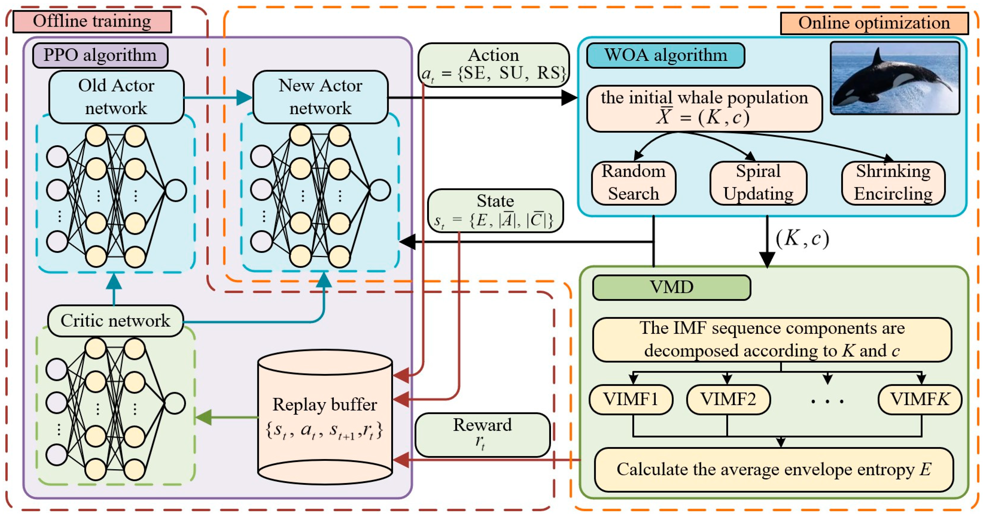
3.3. WOA Based on PPO Algorithm (PWOA)

3.3.1. The PPO Algorithm

The PPO algorithm used in this paper adopts an actor-critic network structure, involving both new and old actor networks along with a critic network, and incorporates an experience buffer for experience replay. In general, RL updates the strategy to maximize the expected value of the rewards by

$$\underset{\theta }{\max }\left(E[{\pi }_{\theta }(u_t|o_t)(q(o_t,u_t)-v^{\varphi }(o_t)]\right)$$

(22)

In the equation, ${\pi }_{\theta }$ represents the policy network at time t; $q(o_t,u_t)$ represents the q value of action $u_t$ taken by RL in state $o_t$; and $v^{\varphi }$ represents the value network at time t.

In order to improve the conventional policy optimization, a time-varying ratio $r_t$ is used to express the change in policy in PPO.

$$r_t={\displaystyle \frac{{\pi }_{\theta }^t(u_t|o_t)}{{\pi }_{\theta }^{t-1}(u_t|o_t)}}$$

(23)

The conventional policy update method is modified by constraint policy update. Constraint policy update was first introduced in the Trust Domain Policy Optimization (TRPO) algorithm to specify the constraint parameter θ, but is soon widely used in the PPO algorithm. The constraints on policy update of PPO are as follows:

$$\underset{\theta }{\max }\left(\underset{\theta }{\min }\left\{r_t(\theta )(q(o_t,u_t)-v^{\varphi }(o_t)),{\widehat{r}}_t(\theta )\right\}\right)$$

(24)

$${\widehat{r}}_t(\theta )=clip(r_t(\theta ),1-ϵ,1+ϵ)$$

(25)

In the equation, ${\widehat{r}}_t$ represents the dynamic change rate of the deviation of the new strategy from the old strategy.

3.3.2. Improve WOA Based on PPO

In the meta-heuristic algorithm, the balance of exploration and utilization is very important to improve the search performance. The actions in the WOA are determined by the agent, including SE, SU, and RS. In this article, the PPO algorithm is applied to model and optimize the behavior decision mechanism of WOA, which enables the agent to choose the most suitable action according to the environment in each iteration. The PWOA can better balance exploration and utilization, avoid premature local optimal solutions, and accelerate convergence. As shown in Figure 2, the main workflow of PWOA’s overall framework includes two stages: offline training and online optimization. During offline training, an optimal behavior decision model is constructed using the PPO. All agents utilize a shared PPO agent for efficient learning, which is conducive to efficient learning of the decision models. In the subsequent stage, the PWOA leverages the trained model to enhance agent behavior, thereby boosting algorithm performance.

3.3.3. Markov Decision Process (MDP) for VMD Parameter Optimization Based on PWOA

MDP is a mathematical framework to describe the discrete time stochastic control processes with Markov properties, which consists of state space, action space, reward function, etc.

• State space: The DRL algorithm’s observed state should supply sufficient information for the agent to make informed behavioral decisions at every iteration. In this article, in order to express the solution state of VMD through PWOA, the concept of envelope entropy is introduced. The envelope entropy reflects the sparsity of the signal, and its magnitude is inversely related to the periodicity of the signal. The greater the signal’s periodicity, the lower the envelope entropy. The average envelope entropy can be mathematically represented as follows:

$$E(\overline{X})=-{\displaystyle \frac{1}{K}}{\displaystyle \sum _{i=1}^K{\displaystyle \sum _{j=1}^m{p}_i}{\log }_2{p}_i}$$

(26)

$$p_i=a(i)/{\displaystyle \sum _{i=1}^{m}a}(i)$$

(27)

$$a(i)=\sqrt{{\left[x(i)\right]}^2+{\left\{H[x(i)]\right\}}^2}$$

(28)

In the equation, $E(\overline{X})$ represents the average envelope entropy of VIMF signal after VMD under current parameters, and K represents the quantity of decomposition modes in VMD; m is the length of VIMF signal; $p_i$ is the signal probability distribution; $a$ is the envelope signal sequence acquired by Hilbert modulation of VIMF signal; and $H[\cdot ]$ represents for Hilbert transform. At the same time, the two fundamental parameters of WOA, $\overline{A}$ and $\overline{C}$, are taken as the elements of the state. Thus, the state can be represented as follows:

$$s_t=\{E, |\overline{A}|, |\overline{C}\left|\right\}$$

(29)

• Action space: In each iteration of PPO, the agent is required to select the next action based on the present state. Likewise, in WOA, the agent must determine its hunting behavior according to the current circumstances. Consequently, the three hunting behaviors of WOA are correlated with the actions of the agent in PPO. Hence, the action space in this study is outlined as follows:

$$a_t=\{\mathrm{SE}, \mathrm{SU}, \mathrm{RS}\}$$

(30)

In the equation, SE is the action of shrinking encircling; SU is the action of the spiral update; and RS is the action of a random exploration.

• Reward function: As the feedback of the environment to the action performed by the agent, it plays a key role in guiding the agent to select the best action. In this paper, the solution with a smaller envelope entropy is more favorable. Therefore, when the agent chooses an update action that reduces the envelope entropy, reward will be carried on; when it increases the envelope entropy, it should be punished. If the action has no effect on the envelope entropy, the reward value is set to zero. In summary, the definition of reward is as follows:

$$r_t=\left\{\begin{array}{l}1 E(\overline{X}(t+1))<E(\overline{X}(t))\\ -1 E(\overline{X}(t+1))>E(\overline{X}(t))\\ 0 E(\overline{X}(t+1))=E(\overline{X}(t))\end{array}\right.$$

(31)

In the equation, $E(\overline{X}(t))$ denotes the average envelope entropy of the present time; and $E(\overline{X}(t+1))$ represents the average envelope entropy after the action.

4. BiGRU Prediction Model

The GRU tackles the problem of gradient vanishing in traditional RNNs. It maintains the memory capacity of LSTM while being more computationally efficient with fewer parameters during training. GRU is equipped with two gates, the reset gate and the update gate, to manage the flow of information. BiGRU is a hybrid model which is optimized and extended by adding a hidden layer on the basis of one-way GRU. The model consists of a forward GRU that accepts a forward input and a reverse GRU that processes a reverse input. Historical data and future data are extracted through two hidden layers and finally eventually linked to the identical output layer. At each time step, the input is concurrently provided to two GRUs in opposing directions, while the output is dictated by two unidirectional GRUs. The structure effectively captures information about the past and future, thereby improving the generalization and accuracy of predictions. The output of BiGRU is $y(t)=[\overrightarrow{h}(t),\overleftarrow{h}(t)]$, where $\overrightarrow{h}(t)$ and $\overleftarrow{h}(t)$ represent the output of the forward and backward GRU layers at the t-th step, respectively. Figure 3 shows the structure of the BiGRU.

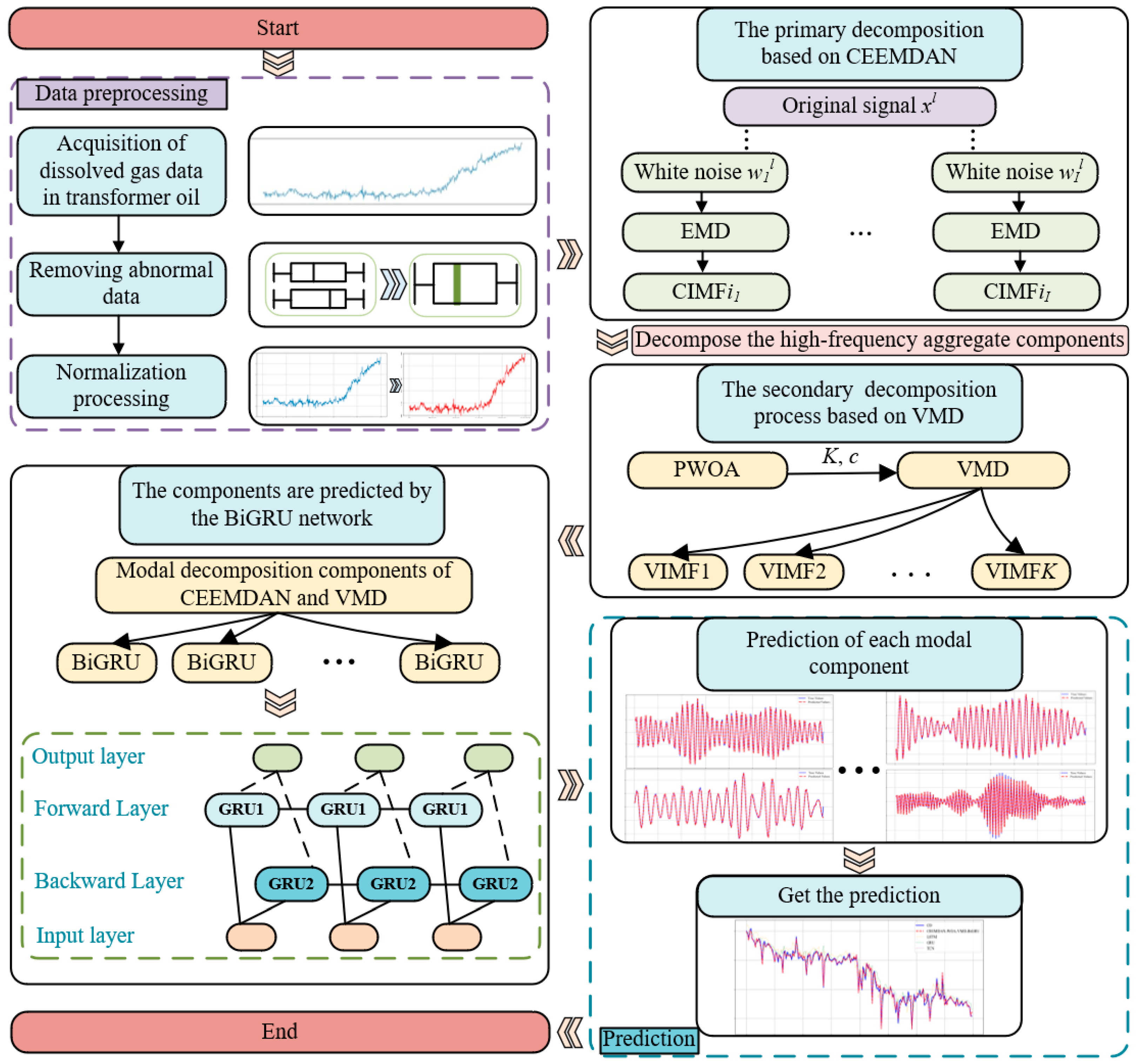
5. Prediction Process of Dissolved Gas in Transformer Oil Based on CEEMDAN-PWOA-VMD-BiGRU

For gas dissolved in transformer oil with significant nonlinearity and instability, the whole framework of the prediction model proposed in this paper based on secondary decomposition is shown in Figure 4.

The specific procedures are outlined below.

• The original data of gas dissolved in the transformer oil are preprocessed, including Z-score outlier detection and linear interpolation. The specific equation is shown as follows:

  $$z_i={\displaystyle \frac{(x_i-\mu )}{\sigma }}$$

  (32)
• In the equation, $z_i$ represents the Z-score, $\mu$ represents the mean, and $\sigma$ represents the standard deviation. If the calculated Z-score exceeds the predefined threshold, the data point is identified as an outlier.
• The preprocessed data is decomposed by CEEMDAN and the subsequences are obtained.
• The quantity of decomposition modes K of VMD and the penalty factor c are obtained by the PWOA, then the highly complex components of the subsequence are aggregated for VMD secondary decomposition to obtain the stable subsequence.
• The decomposition components of CEEMDAN and VMD are normalized.

  $$x_i^{\prime }={\displaystyle \frac{x_i-x_{\min }}{x_{\max }-x_{\min }}}$$

  (33)
• In the equation, $x_i^{\prime }$ represents the normalized value of $x_i$; and $x_{\max }$ and $x_{\min }$ represent the maximum and minimum values, respectively.
• The normalized data is sent to the BiGRU for forecasting, and the predictions of each component are combined to obtain the ultimate forecast results.

6. Case Study Analysis

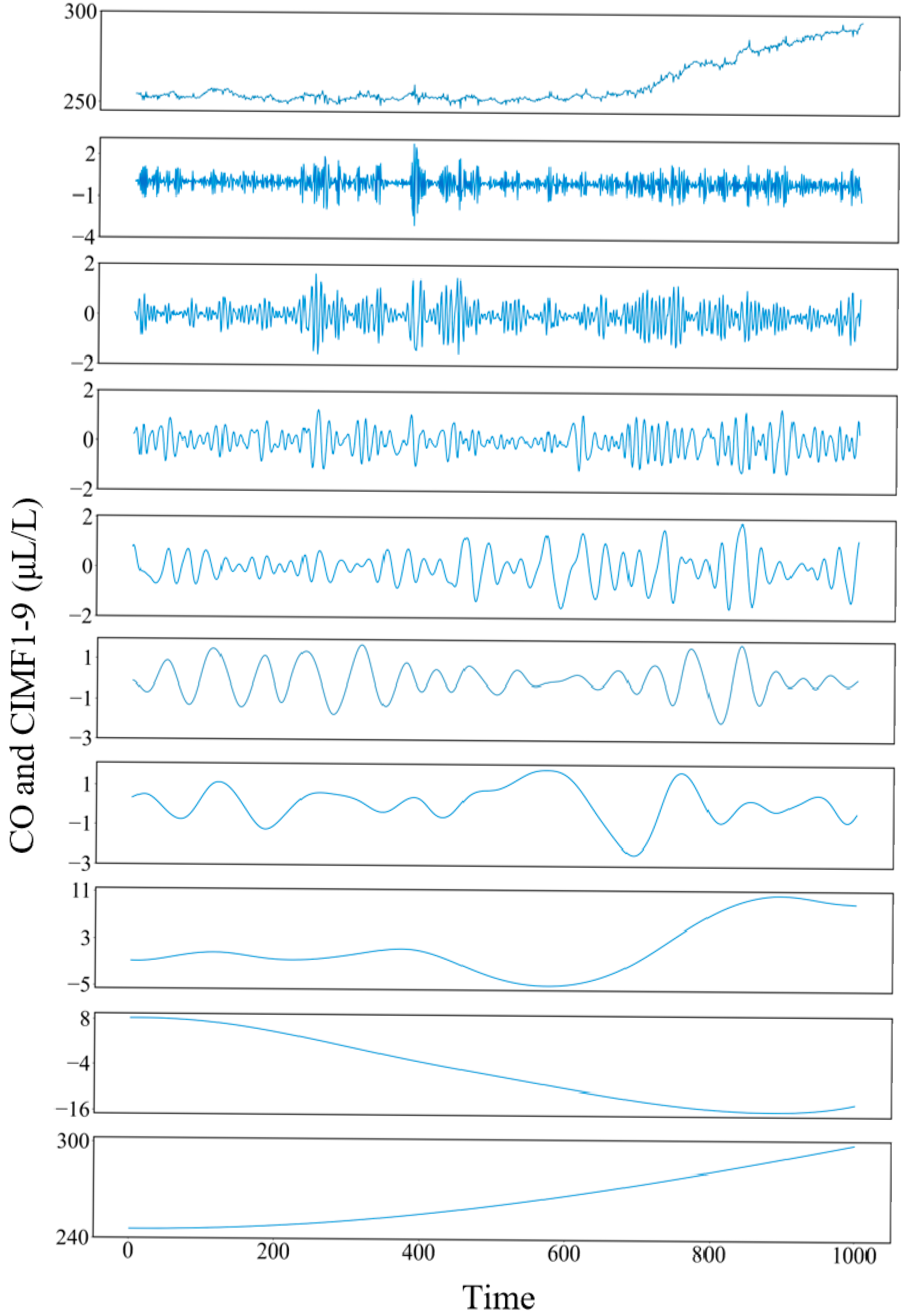
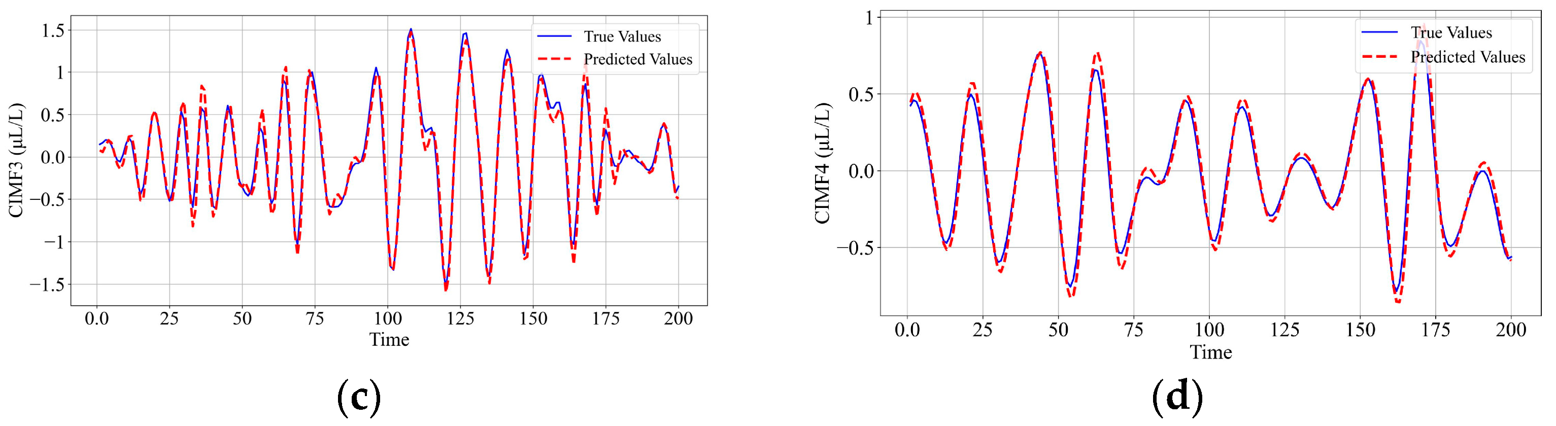
6.1. CEEMDAN Decomposition of Gas Sequences

First, CEEMDAN decomposition is applied to the CO gas sequence, and adaptively the original sequence is decomposed into nine CIMF components, as shown in Figure 5. Sample Entropy is a complexity measure means used in time series analysis which quantifies the intricacy of the signal [27]. As the Sample Entropy increases, the time sequences become more complex or irregular; on the other hand, a lower Sample Entropy indicates a more regular sequence. In this paper, the Sample Entropy values of each CIMF component are calculated, and the results are displayed in

Table 1. Sample Entropy of modal components from CEEMDAN decomposition.

Decomposed Components	Sample Entropy	Decomposed Components	Sample Entropy
CO	1.9592	CIMF5	0.3627
CIMF1	1.1647	CIMF6	0.2244
CIMF2	0.7338	CIMF7	0.1778
CIMF3	0.5542	CIMF8	0.1886
CIMF4	0.5075	CIMF9	0.010

. By analyzing the shapes of the component curves in Figure 5 in conjunction with the results in Table 1, it can be found that, after CEEMDAN decomposition, in comparison with the original sequence, the complexity of each modal component has decreased. The Sample Entropy of CIMF1-CIMF4 is relatively higher than that of other components. Predictions are made for the components with higher Sample Entropy, and the results are displayed in Figure 6. The predictive accuracy of the higher-complexity components, CIMF1 and CIMF2, is evidently worse than that of CIMF3 and CIMF4, which indicates that some high-frequency components like CIMF1 and CIMF2 after CEEMDAN decomposition still retain significant complexity and irregularity. Direct prediction of these components results in unsatisfactory results, which constitute the primary source of prediction error in the final prediction caused by the combination of the individual component predictions.

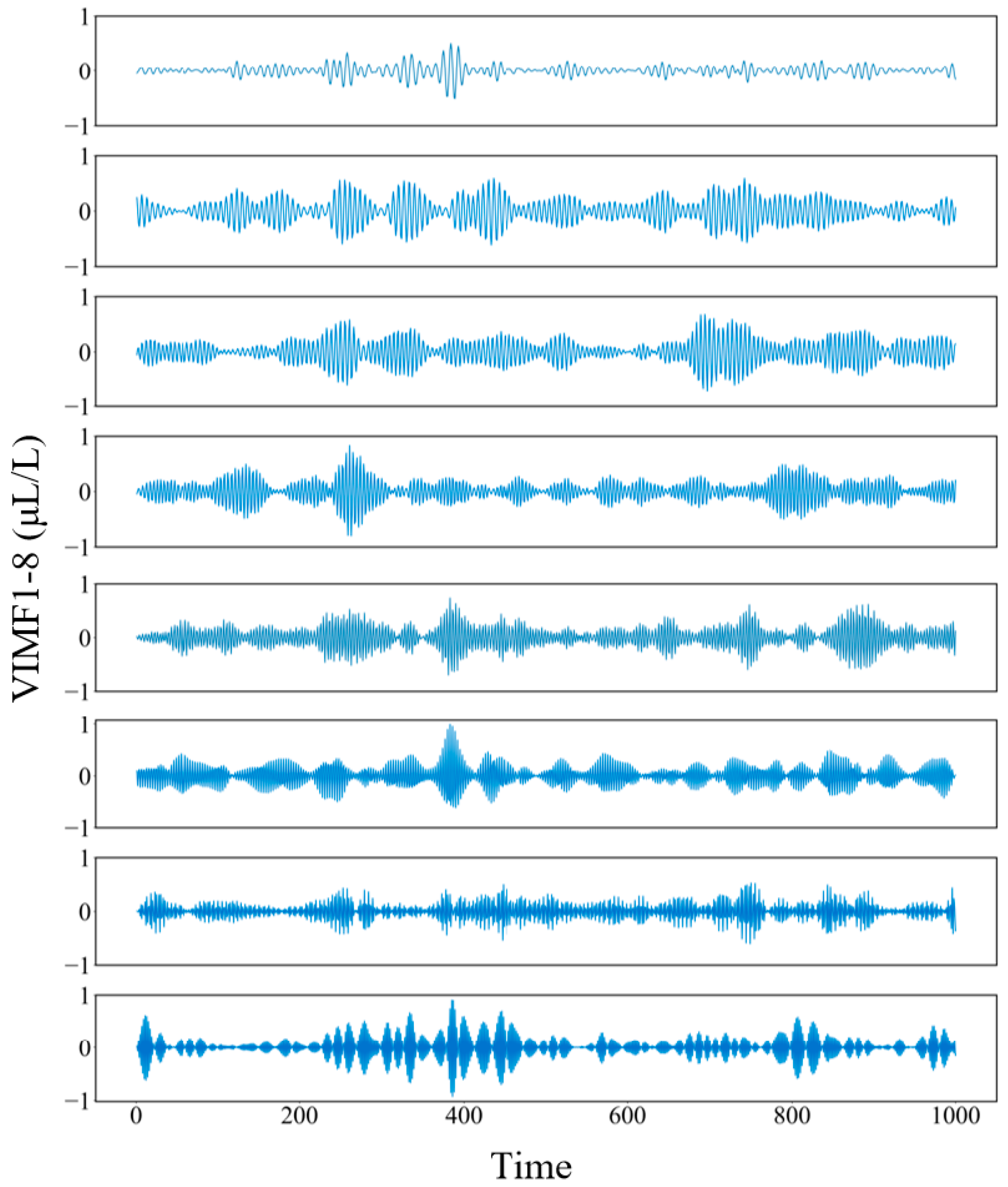
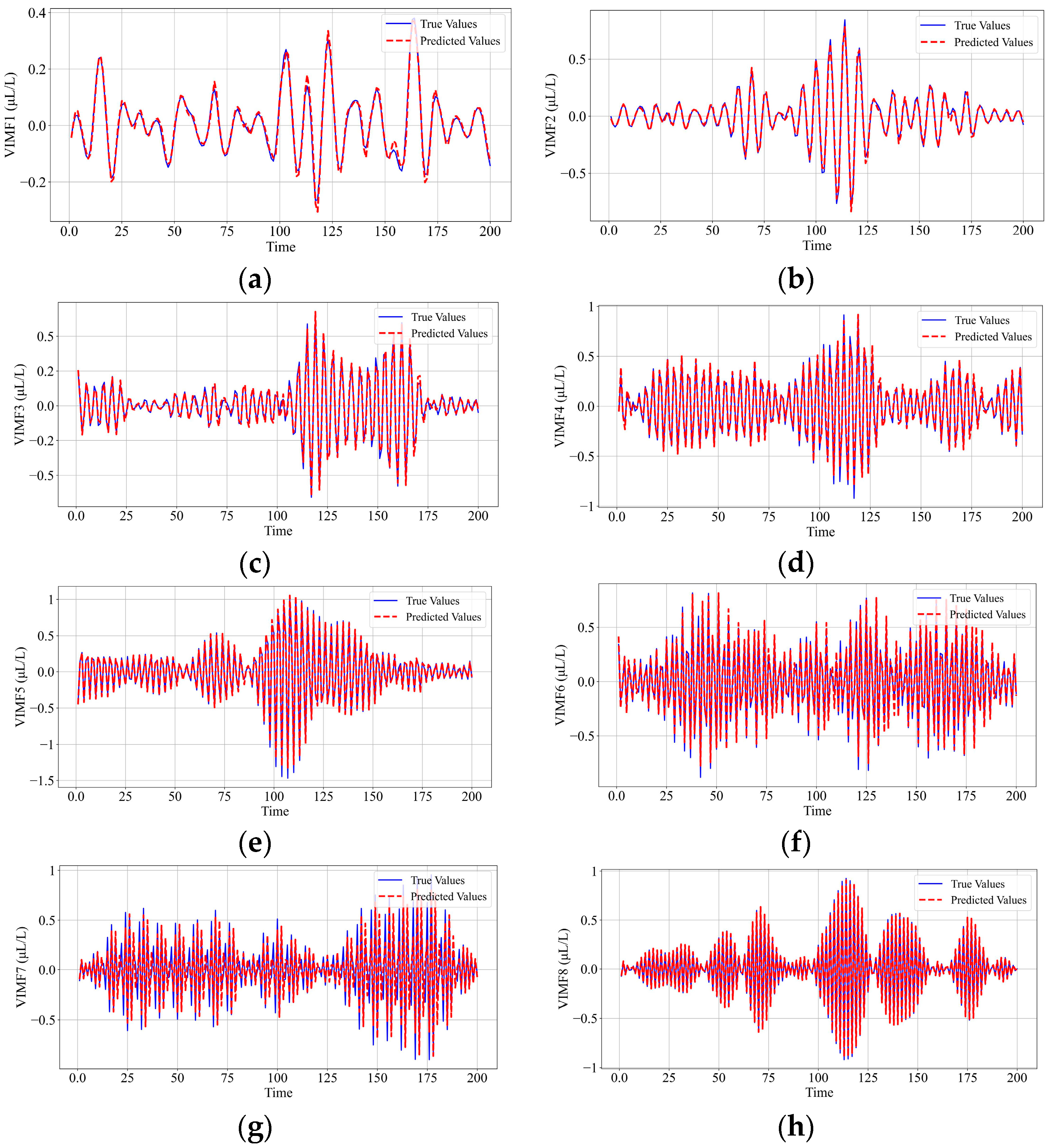
6.2. Secondary Decomposition by VMD of Gas Sequences

If CIMF1 and CIMF2 of CEEMDAN decomposition cannot fit the requirements, CIMF1 and CIMF2 are combined and VMD secondary decomposition is performed and multiple stationary components of further decomposition are obtained. Then BiGRU was used to predict each component. The setting of the VMD hyperparameters significantly influences the decomposition results; therefore, the PWOA is employed to obtain an optimized value of the decomposition mode K and the penalty factor c. Specifically, K = 8 and c = 2695.32 in this study. The decomposed VIMF components are displayed in Figure 7, and the prediction results generated by BiGRU are presented in Figure 8. The Sample Entropy values of each component are provided in

Table 2. Sample Entropy of modal components from VMD.

Decomposed Components	Sample Entropy	Decomposed Components	Sample Entropy
VIMF1	0.1783	VIMF5	0.1318
VIMF2	0.2817	VIMF6	0.2717
VIMF3	0.1934	VIMF7	0.3559
VIMF4	0.0914	VIMF8	0.1836

. As shown in Figure 7 and Figure 8 and Table 2, the complexity of the original high-complexity components is significantly reduced after secondary decomposition, and the prediction performance of each component is notably improved.

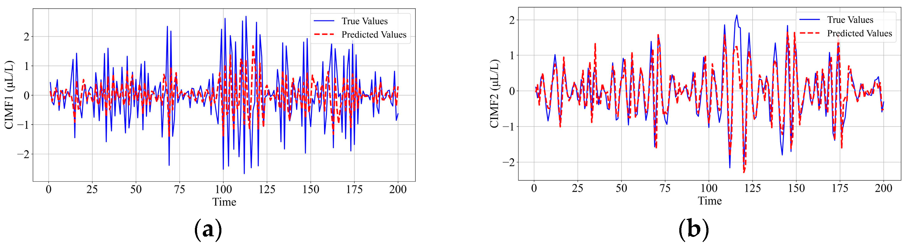
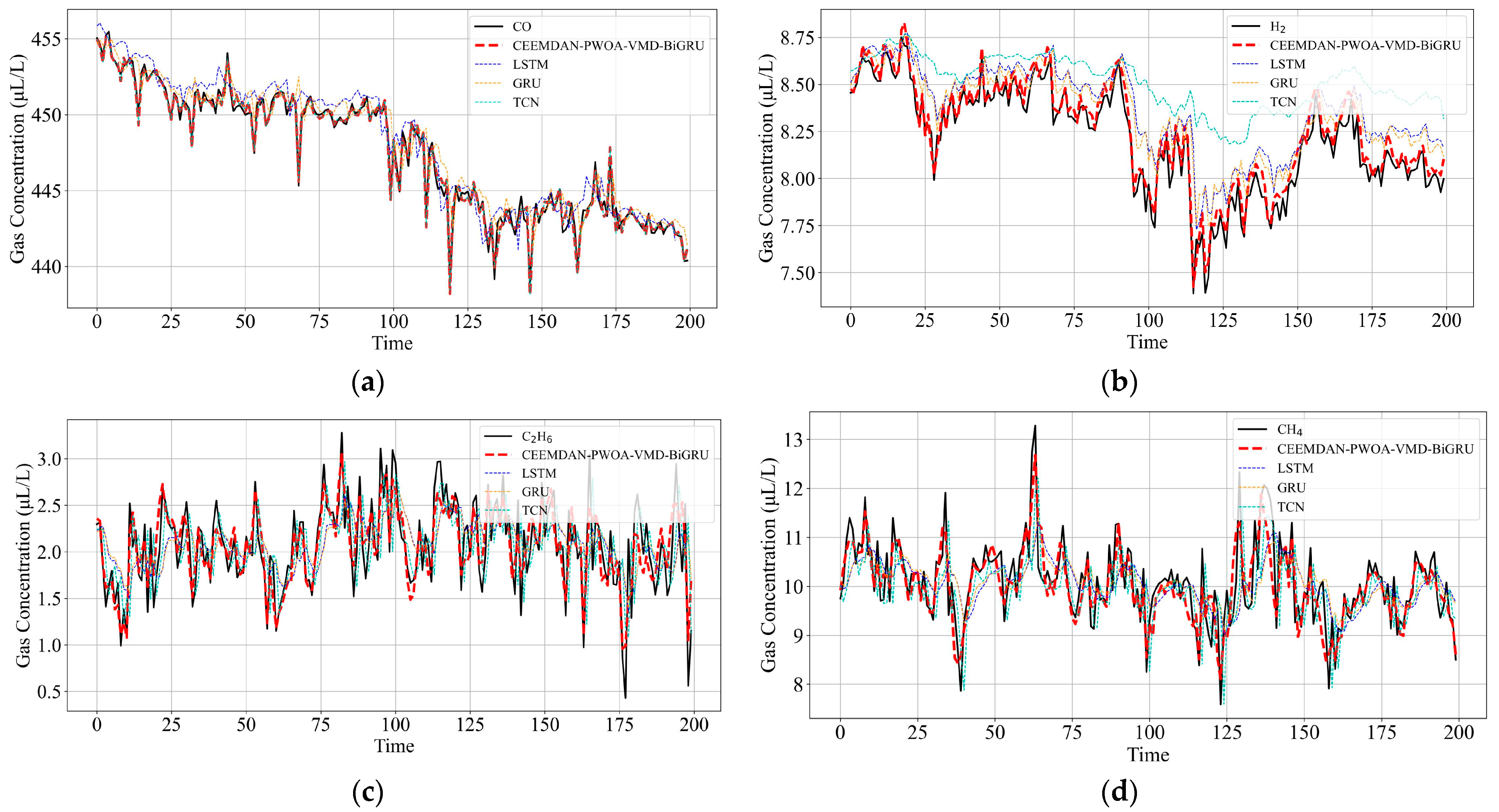
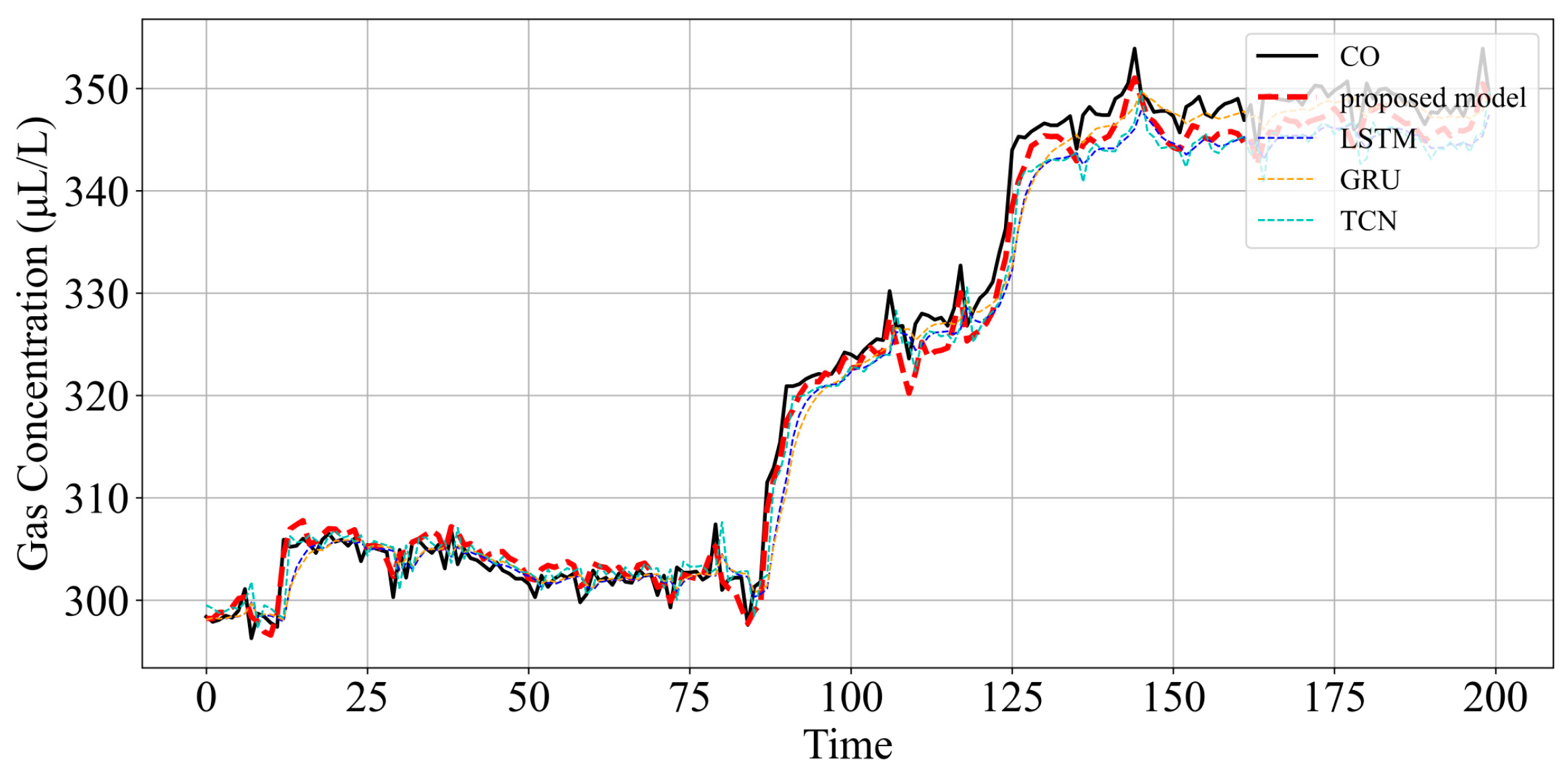
6.3. Analysis and Comparison of Testing Results

To validate the efficacy of the proposed approach, we implement in CO, H₂, C₂H₆, and CH₄ gas sequences to derive the ultimate prediction results. The experimental data are derived from the oil chromatograph data continuously monitored at a 110 kV substation of State Grid Shanxi Electric Power Company (Jincheng, China). The sampling period of the dataset is 6 h, containing a total of 1000 time steps, and the dataset is segmented in a ratio of 4:1. These results are then contrasted with traditional models such as LSTM, GRU, and TCN. The model parameters used in the experiment are shown in

Table 3. The parameters of the models.

Algorithm Type	Parameters
CEEMDAN	Trials = 100, noise strength = 0.2
TCN	Hidden dim = 8, hidden layers = 3, kernel size = 3, stride = 1, padding = 2, Adam optimizer, lr = 0.01
GRU	Hidden dim = 256, hidden layers = 1, Adam optimizer, lr = 0.01
LSTM	Hidden dim = 64, hidden layers = 1, Adam optimizer, lr = 0.01
BiGRU	Hidden dim = 84, hidden layers = 1, Adam optimizer, lr = 0.01

. The input length of each model is 20. The prediction curves are shown in Figure 9, and the prediction errors are presented in

Table 4. The predictive performance of different models.

Model Type	CO		H2		C2H6		CH4
	MAE (%)	MSE (%)	MAE (%)	MSE (%)	MAE (%)	MSE (%)	MAE (%)	MSE (%)
proposed model	3.64	2.18	0.54	0.05	1.92	0.58	3.25	1.86
LSTM	10.44	25.16	1.62	0.39	3.55	2.06	5.68	5.63
GRU	11.09	26.61	1.41	0.32	3.56	2.04	5.60	5.55
TCN	9.33	11.89	3.03	1.25	3.78	2.34	5.91	6.15

. As it can be observed in Figure 9, when predicting gas sequences with low stability and high complexity, models such as LSTM, GRU and TCN perform poorly, as they only capture the basic trend of the original sequence and show poor fitting performance on the fluctuating parts. In contrast, the proposed CEEMDAN-PWOA-VMD-BiGRU model demonstrates better predictive performance on the fluctuations of the gas sequences. As shown in Table 4, taking CO as an example, the MAE of the model proposed in this paper is reduced by 6.88%, 7.45%, and 5.69%, respectively, compared with traditional algorithms such as LSTM, GRU, and TCN.

6.4. Experiment Analysis of Samples with Abnormal Change Trend

Take a certain part in the dataset where the concentrations of CO increase significantly. To validate the proposed model’s ability of tracking the gas changes under abnormal conditions, prediction experiments were conducted on the CO gas sequence using the trained CEEMDAN-PWOA-VMD-BiGRU, LSTM, GRU, and TCN. The prediction curves are shown in Figure 10, and the prediction errors are presented in

Table 5. The predictive performance of different models for abnormally changing gas of CO.

Type of Model	MAE (%)	MSE (%)
proposed model	3.00	0.125
LSTM	4.34	0.326
GRU	3.07	0.210
TCN	4.47	0.314

.

As shown in Figure 10 and Table 5, from time step 0 to 75, the gas sequence remains relatively stable, followed by a sharp increase to 350 μL/L. The prediction curves of all four models generally follow the trend of the change. Among them, the proposed model demonstrates the best performance in terms of the prediction error. Compared with the GRU, LSTM, and TCN models, the proposed model tracks the fluctuations of the CO sequence best.

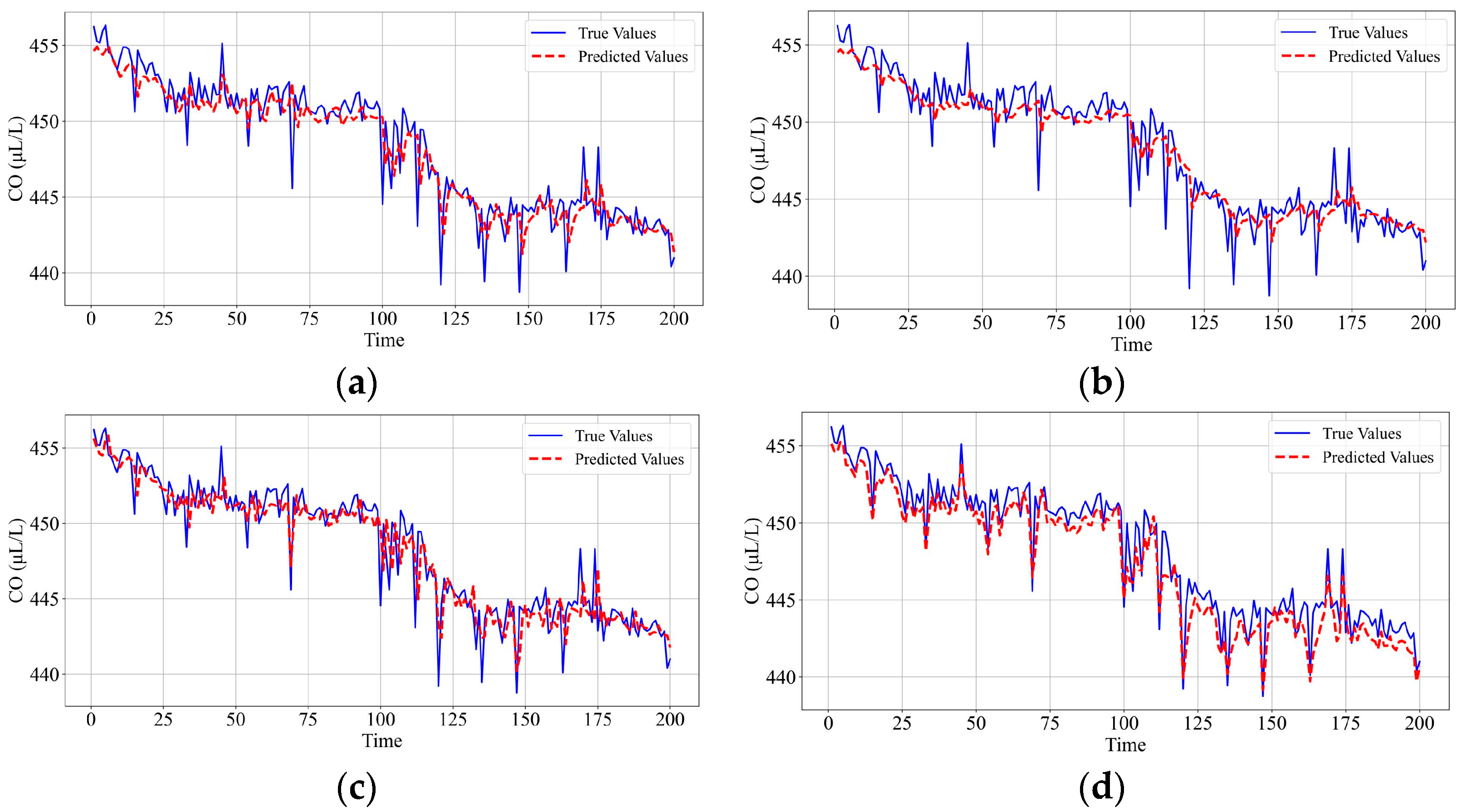
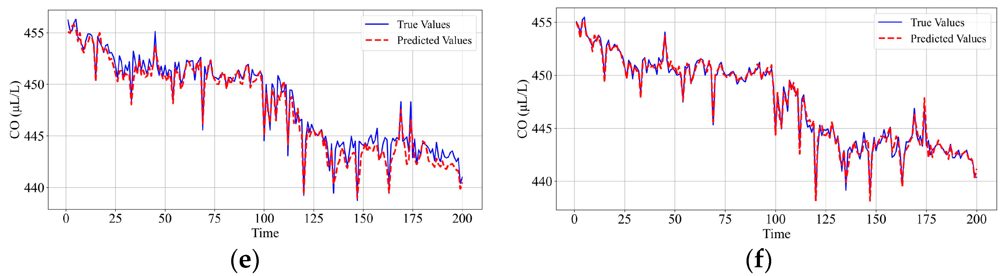
6.5. Ablation Study of the Prediction

To further assess the contribution of the proposed model in the improvement of the accuracy, an ablation study was conducted. Using CO as an example, the prediction and errors are presented in Figure 11 and

Table 6. Prediction performance of different models for CO concentration.

Model Type	MAE (%)	MSE (%)
BiGRU	11.06	25.60
VMD-BiGRU	16.86	36.81
CEEMDAN-BiGRU	9.46	15.43
CEEMDAN-VMD-BiGRU	8.47	12.65
CEEMDAN-WOA-VMD-BiGRU	6.13	7.85
proposed model	3.64	2.18

, respectively. The default hyperparameter settings for VMD are K = 3 and c = 2000.

According to Table 6 and Figure 11, the MAE and MSE of the CEEMDAN-BiGRU model are 1.6% and 10.17% lower than that of the BiGRU model, respectively, while the MAE and MSE of the VMD-BiGRU model increased. It indicates that modal decomposition leads to enhanced prediction accuracy, but the improper setting of VMD parameters may lead to poor prediction results. Compared with the CEEMDAN-BiGRU model and the VMD-BiGRU model, the MAE of the CEEMDAN-VMD-BiGRU model decreased by 0.99% and 8.39%, respectively, indicating that the prediction accuracy could be further improved by quadratic decomposition. Compared with the CEEMDAN-VMD-BiGRU model and the CEEMDAN-WOA-VMD-BiGRU model, the MAE of the model proposed in this paper decreases by 4.83% and 2.49%, respectively. It can be inferred that parameter optimization of VMD through WOA can solve the problem of the poor prediction effect caused by the subjective setting of the parameters. From the MAE and MSE of the proposed method, it obviously shows that PPO promotes WOA in parameter optimization, avoiding falling into local optimal and achieving adaptive parameter settings for VMD, which further improve the prediction accuracy, even in gas fluctuation situations.

7. Conclusions

To enhance the accuracy of predicting gas content in transformer oil, a method based on CEEMDAN-PWOA-VMD and BiGRU are proposed. Firstly, CEEMDAN is employed for mode decomposition. To address the large prediction errors caused by the strong nonlinear characteristics of the high-frequency modal components, VMD is introduced for secondary decomposition. Although VMD provides a more refined decomposition, the selection of the optimal decomposition number and secondary penalty factor involves subjective judgment, which introduces uncertainty. Therefore, WOA is applied to optimize the VMD parameter settings. To further enhance the consistency and effectiveness of the decomposition, PPO is adopted to optimize the search process of WOA, which significantly enhances the optimization effect and achieves a more accurate and stable secondary decomposition. Subsequently, BiGRU is employed for training, which better captures the time series features and the trend of variations. Finally, reconstructing the predictions of each component leads to enhanced prediction accuracy. Experimental results indicate that the proposed algorithm enhances the precision, effectively addressing the nonlinear challenges posed by the high-frequency modal components and the issues related to subjective setting of the parameters. And based on the presented gas prediction, an online monitoring system and its application will be considered in a future study.

References

1. Herath, T.; Wang, Z.D.; Liu, Q.; Wilson, G.; Hooton, R.; Raymond, T. Development of Trend Detection Technique for Dissolved Gas Analysis of Transmission Power Transformers. IEEE Trans. Power Deliv. 2025, 40, 332–342. [Google Scholar] [CrossRef]
2. Guerbas, F.; Benmahamed, Y.; Teguar, Y.; Dahmani, R.A.; Teguar, M.; Ali, E.; Bajaj, M.; Dost Mohammadi, S.A.; Ghoneim, S.S.M. Neural Networks and Particle Swarm for Transformer Oil Diagnosis by Dissolved Gas Analysis. Sci. Rep. 2024, 14, 9271. [Google Scholar] [CrossRef] [PubMed]
3. Jin, L.; Kim, D.; Chan, K.Y.; Abu-Siada, A. Deep Machine Learning-Based Asset Management Approach for Oil- Immersed Power Transformers Using Dissolved Gas Analysis. IEEE Access 2024, 12, 27794–27809. [Google Scholar] [CrossRef]
4. Pereira, F.H.; Bezerra, F.E.; Junior, S.; Santos, J.; Chabu, I.; Souza, G.F.M.d.; Micerino, F.; Nabeta, S.I. Nonlinear Autoregressive Neural Network Models for Prediction of Transformer Oil-Dissolved Gas Concentrations. Energies 2018, 11, 1691. [Google Scholar] [CrossRef]
5. Elânio Bezerra, F.; Zemuner Garcia, F.A.; Ikuyo Nabeta, S.; Martha de Souza, G.F.; Chabu, I.E.; Santos, J.C.; Junior, S.N.; Pereira, F.H. Wavelet-Like Transform to Optimize the Order of an Autoregressive Neural Network Model to Predict the Dissolved Gas Concentration in Power Transformer Oil from Sensor Data. Sensors 2020, 20, 2730. [Google Scholar] [CrossRef]
6. Lu, S.X.; Lin, G.; Que, H.; Li, M.J.J.; Wei, C.H.; Wang, J.K. Grey Relational Analysis Using Gaussian Process Regression Method for Dissolved Gas Concentration Prediction. Int. J. Mach. Learn. Cybern. 2019, 10, 1313–1322. [Google Scholar] [CrossRef]
7. Xing, Z.; He, Y.; Wang, X.; Shao, K.; Duan, J. VMD-IARIMA-Based Time-Series Forecasting Model and Its Application in Dissolved Gas Analysis. IEEE Trans. Dielectr. Electr. Insul. 2023, 30, 802–811. [Google Scholar] [CrossRef]
8. Wei, C.; Tang, W.; Wu, Q. Dissolved Gas Analysis Method Based on Novel Feature Prioritisation and Support Vector Machine. IET Electr. Power Appl. 2014, 8, 320–328. [Google Scholar] [CrossRef]
9. He, J.; Huang, L.; Xiao, Y.; Li, W.; Yin, J.; Duan, Q.; Wei, L. Prediction Model of Continuous Discharge Coefficient from Tank Based on KPCA-DE-SVR. J. Loss Prev. Process Ind. 2024, 89, 105316. [Google Scholar] [CrossRef]
10. Ma, Z.; Zhang, H.; Liu, J. MM-RNN: A Multimodal RNN for Precipitation Nowcasting. IEEE Trans. Geosci. Remote Sens. 2023, 61, 4101914. [Google Scholar] [CrossRef]
11. Chen, T.; Guo, S.; Zhang, Z.; Yuan, Y.; Gao, J. A Method for Predicting Transformer Oil-Dissolved Gas Concentration Based on Multi-Window Stepwise Decomposition with HP-SSA-VMD-LSTM. Electronics 2024, 13, 2881. [Google Scholar] [CrossRef]
12. Wang, S.; Shi, J.; Yang, W.; Yin, Q. High and Low Frequency Wind Power Prediction Based on Transformer and BiGRU-Attention. Energy 2024, 288, 129753. [Google Scholar] [CrossRef]
13. Heddam, S.; Al-Areeq, A.M.; Tan, M.L.; Ahmadianfar, I.; Halder, B.; Demir, V.; Kilinc, H.C.; Abba, S.I.; Oudah, A.Y.; Yaseen, Z.M. New Formulation for Predicting Total Dissolved Gas Supersaturation in Dam Reservoir: Application of Hybrid Artificial Intelligence Models Based on Multiple Signal Decomposition. Artif. Intell. Rev. 2024, 57, 85. [Google Scholar] [CrossRef]
14. Coşkun, M.; Gürüler, H.; Istanbullu, A.; Peker, M. Determining the Appropriate Amount of Anesthetic Gas Using DWT and EMD Combined with Neural Network. J. Med. Syst. 2015, 39, 173. [Google Scholar] [CrossRef]
15. Heddam, S.; Vishwakarma, D.K.; Abed, S.A.; Sharma, P.; Al-Ansari, N.; Alataway, A.; Dewidar, A.Z.; Mattar, M.A. Hybrid River Stage Forecasting Based on Machine Learning with Empirical Mode Decomposition. Appl. Water Sci. 2024, 14, 46. [Google Scholar] [CrossRef]
16. Melalkia, L.; Berrezzek, F.; Khelil, K.; Saim, A.; Nebili, R. A Hybrid Error Correction Method Based on EEMD and ConvLSTM for Offshore Wind Power Forecasting. Ocean Eng. 2025, 325, 120773. [Google Scholar] [CrossRef]
17. Sahu, P.K.; Rai, R.N.; Patel, N. Deep Learning-Based Fault Classification of Rolling Bearings under Noisy Conditions Using CEEMD-VMD-IMF with Magnitude Scalogram Images. J. Mech. Sci. Technol. 2024, 38, 5281–5295. [Google Scholar] [CrossRef]
18. Naraiah, R.P.; Kumar, P.N.; Dey, A. GNSS Multipath Error Analysis Based on Improved CEEMDAN and Detrended Fluctuation Analysis. J. Indian Soc. Remote Sens. 2025. [Google Scholar] [CrossRef]
19. Ni, L.; Khim-Sen Liew, V. Carbon Emission Price Forecasting in China Using a Novel Secondary Decomposition Hybrid Model of CEEMD-SE-VMD-LSTM. Syst. Sci. Control Eng. 2024, 12, 2291409. [Google Scholar] [CrossRef]
20. Sun, W.; Huang, C. A Carbon Price Prediction Model Based on Secondary Decomposition Algorithm and Optimized Back Propagation Neural Network. J. Clean. Prod. 2020, 243, 118671. [Google Scholar] [CrossRef]
21. Zhao, Y.; Li, H. A Denoising and Recognition Matching Algorithm of Projectile Signal in Infrared Light Screens Based on HOA-VMD. Microw. Opt. Technol. Lett. 2025, 67, e70166. [Google Scholar] [CrossRef]
22. Li, Y.; Ding, Z.; Yu, Y.; Liu, Y. Hybrid Energy Storage Power Allocation Strategy Based on Parameter-Optimized VMD Algorithm for Marine Micro Gas Turbine Power System. J. Energy Storage 2023, 73, 109189. [Google Scholar] [CrossRef]
23. Samantaray, S.; Sahoo, A. Prediction of Suspended Sediment Concentration Using Hybrid SVM-WOA Approaches. Geocarto Int. 2022, 37, 5609–5635. [Google Scholar] [CrossRef]
24. Uzer, M.S.; Inan, O. Application of Improved Hybrid Whale Optimization Algorithm to Optimization Problems. Neural Comput. Appl. 2023, 35, 12433–12451. [Google Scholar] [CrossRef]
25. Singh, B.; Kumar, R.; Singh, V.P. Reinforcement Learning in Robotic Applications: A Comprehensive Survey. Artif. Intell. Rev. 2022, 55, 945–990. [Google Scholar] [CrossRef]
26. Yu, C.; Velu, A.; Vinitsky, E.; Gao, J.; Wang, Y.; Bayen, A.; Wu, Y. The Surprising Effectiveness of PPO in Cooperative, Multi-Agent Games. arXiv 2022, arXiv:2103.01955. [Google Scholar]
27. Ardila-Rey, J.; Rivera-Caballero, O.; Boya, C. Sample Entropy as a Performance Indicator of UHF Real Signal Denoising from Partial Discharges. IEEE Trans. Dielectr. Electr. Insul. 2025, 32, 1333–1342. [Google Scholar] [CrossRef]
Figure 1. Flowchart of primary mode decomposition based on CEEMDAN.
Electronics 14 02370 g001
Figure 2. Flowchart of secondary mode decomposition based on PWOA-VMD.
Electronics 14 02370 g002
Figure 3. Structure diagram of BiGRU.
Electronics 14 02370 g003
Figure 4. Flowchart of dissolved gas prediction model in transformer oil.
Electronics 14 02370 g004
Figure 5. Modal components obtained from CEEMDAN decomposition.
Electronics 14 02370 g005
Figure 6. Prediction results of CIMF1 to CIMF4: (a) CIMF1; (b) CIMF2; (c) CIMF3; (d) CIMF4.
Electronics 14 02370 g006aElectronics 14 02370 g006b
Figure 7. Modal components obtained from VMD.
Electronics 14 02370 g007
Figure 8. Prediction results of modal components obtained from VMD: (a) VIMF1; (b) VIMF2; (c) VIMF3; (d) VIMF4; (e) VIMF5; (f) VIMF6; (g) VIMF7; (h) VIMF8.
Electronics 14 02370 g008
Figure 9. Comparison of gas prediction results of different models. (a) CO; (b) H2; (c) C2H6; (d) CH4.
Electronics 14 02370 g009
Figure 10. The prediction results of different models for abnormally changing gas of CO.
Electronics 14 02370 g010
Figure 11. Comparison of the CO prediction results of each model: (a) BiGRU; (b) VMD-BiGRU; (c) CEEMDAN-BiGRU; (d) CEEMDAN-VMD-BiGRU; (e) CEEMDAN-WOA-VMD-BiGRU; (f) proposed model.
Electronics 14 02370 g011aElectronics 14 02370 g011b