Optimizing Home Energy Flows and Battery Management with Supervised and Unsupervised Learning in Renewable Systems

Abstract

This study examines reinforcement learning (RL) and fuzzy logic control (FLC) for optimizing battery energy storage in residential systems with photovoltaic (PV) power, grid interconnection, and dynamic or fixed electricity pricing. Effective management strategies are crucial for reducing costs, extending battery lifespan, and ensuring reliability under fluctuating demand and tariffs. A 24 h simulation with minute-level resolution modeled diverse conditions, including random household demand and ten initial state of charge (SOC) levels from 0% to 100%. RL employed proximal policy optimization (PPO) for adaptive energy scheduling, while FLC used rule-based logic for charge–discharge cycles. Results showed that FLC rapidly restored SOC at low levels, ensuring immediate availability but causing cost fluctuations and increased cycling, particularly under stable pricing or low demand. RL dynamically adjusted charging and discharging, reducing costs and smoothing energy flows while limiting battery cycling. Feature importance analysis using multiple linear regression (MLR) and random forest regression (RFR) confirmed SOC and time as key performance determinants. The findings highlight a trade-off between FLC’s rapid response and RL’s sustained cost efficiency, providing insights for optimizing residential energy management to enhance economic and operational performance.

1. Introduction

In recent years, energy management in residential environments has become increasingly complex due to the growing integration of renewable energy sources (RESs) and advancements in energy technologies [1]. The residential sector, accounting for approximately 27% of global energy consumption, is crucial in global efforts to improve energy efficiency and reduce greenhouse gas emissions [2,3]. Smart homes, equipped with technologies such as photovoltaic (PV) panels, energy storage systems (ESSs), and smart appliances, offer opportunities for more efficient energy management by balancing energy generation and consumption, reducing costs, and improving sustainability [4,5].

The optimization of ESSs, which stores surplus energy generated by RESs, presents a significant challenge in smart home energy management [6]. These systems play a vital role in mitigating the variability of RESs by storing excess energy for later use, ensuring energy availability during periods of low generation or high demand. However, their operation is complicated by the fluctuating nature of RESs, particularly solar and wind, combined with variable household demand, which requires sophisticated control strategies to manage these systems efficiently [7]. Traditional methods, such as rule-based systems and Mixed-Integer Linear Programming (MILP), often struggle to adapt to the real-time variability of these dynamic environments due to their reliance on static models [8]. This limitation underscores the necessity for advanced methodologies to overcome these challenges and improve system performance.

RL has emerged as a promising solution to these challenges, enabling systems to autonomously learn optimal control policies through continuous interaction with their environment [9,10]. RL-based systems dynamically adjust their control strategies based on real-time data, making them well-suited for managing the complexity and variability inherent in energy systems [11,12]. Among RL algorithms, Proximal Policy Optimization (PPO) was selected due to its balance between stability and adaptability. Unlike the Deep Deterministic Policy Gradient (DDPG), which requires extensive hyper-parameter tuning and is sensitive to small changes in training conditions, PPO ensures steady learning progress through its trust-region update mechanism. Compared to SAC, which offers strong performance but requires significantly higher computational resources due to entropy maximization, PPO provides an efficient and computationally feasible approach for real-time energy management. These advantages make PPO particularly well-suited for optimizing charge and discharge actions under fluctuating electricity prices and demand [13].

As examples, Vázquez-Canteli and Nagy (2019) demonstrated that RL-based systems can achieve up to a 31.5% reduction in household electricity costs by dynamically adjusting energy consumption based on fluctuating prices [14]. Similarly, Lee and Choi (2019) applied Q-learning to optimize household appliances and ESS, achieving a 14% reduction in energy costs [15]. These findings underline RL’s potential to transform energy management systems through adaptability and real-time optimization. Furthermore, the ability to autonomously update decision-making frameworks based on evolving market and demand conditions makes RL particularly suitable for residential energy systems.

FLC has traditionally been used in energy management systems where precise models are unavailable [16,17,18,19]. FLC uses predefined linguistic rules to make decisions based on imprecise inputs, enabling it to manage non-linear systems effectively. This rule-based approach has effectively managed straightforward, well-defined energy systems, offering simplicity and computational efficiency. While FLC performs well in predictable and stable environments, its reliance on fixed rules often limits its ability to adapt to dynamic and real-time energy supply and demand [20]. Shaqour and Hagishima (2022) reviewed FLC applications, highlighting their practical uses in managing simpler energy systems. However, its limitations in more dynamic scenarios were also noted [21]. While FLC excels in more straightforward, more predictable environments where computational simplicity is valued, its performance diminishes as the complexity of the energy system increases.

In contrast, RL continuously adapts to new strategies based on real-time data, making it more flexible for dynamic residential energy environments. Advanced techniques such as Deep Reinforcement Learning (DRL) enhance RL’s capacity to manage large datasets and more complex decision-making processes [22]. Cui et al. (2023) demonstrated that DRL-based systems can effectively manage multi-energy microgrids, significantly improving system efficiency and reducing costs [23]. In addition to these developments, multi-agent reinforcement learning (MARL) holds the potential to coordinate multiple energy resources, including PV systems, ESSs, and electric vehicles (EVs). By aligning the operation of various components within the energy system, MARL can ensure efficient energy allocation while minimizing operational costs.

MARL also holds the potential to coordinate multiple energy resources, including PV systems, ESSs, and EVs [24,25,26]. Xu et al. (2024) applied MARL to hybrid power systems, achieving substantial cost reductions while improving energy efficiency [27,28]. EVs can act as mobile energy storage units, charging when excess energy is available and discharging during peak demand. Tang et al. [29] explored this additional layer of flexibility. They demonstrated how RL-based methods improved system resilience and reduced energy costs in hybrid power systems. Moreover, Lu et al. [30] modeled the aggregation and competition process of ESS and PV units within a multi-ESP VPP framework, capturing the dynamic interactions between energy service providers and distributed energy resources. The results demonstrate MARL’s potential in optimizing resource management, improving payoff allocations, and enhancing DER participation in VPPs. These studies illustrate RL approaches’ growing versatility and scalability, particularly when integrated with multi-component systems in residential energy applications.

In addition, Liu et al. (2022) proposed a multi-objective RL framework for microgrid energy management, highlighting the ability of RL to address both economic and environmental objectives in residential systems [31]. Bose et al. (2021) examined RL’s application in local energy markets, showing how autonomous agents can optimize energy consumption and grid interaction [32]. Finally, Wu et al. (2018) explored continuous RL for energy management in hybrid electric buses, illustrating RL’s broad applicability across various sectors, including transportation [33]. These diverse applications underscore RL’s transformative potential in addressing energy management challenges in residential and broader energy systems.

The RL model in this study observes key variables such as the battery’s SOC, PV power generation, load demand, grid interaction, and electricity prices. These observations form a six-dimensional input vector the RL agent uses to determine optimal charging or discharging actions for the ESS. The system minimizes electricity costs while maintaining SOC within desired limits. The battery has a capacity of 40,000 Wh, and actions range between −5000 W and 5000 W, representing charging or discharging power. RL-based systems reduce costs while maintaining reliability by avoiding grid electricity during peak prices and maximizing stored solar energy use.

Managing electricity costs is a key challenge in residential energy systems, particularly under variable pricing structures. This study evaluated RL and FLC models using a tiered electricity pricing model based on Jordan’s official 2024 tariff structure. The pricing structure introduces cost variations based on energy consumption levels, influencing the decision-making process of the controllers. The study also considers seasonal and weekly demand variations to simulate real-world energy use conditions, ensuring that the optimization strategies developed are practical and applicable.

However, several challenges arise when implementing RL-based systems. Accurately modeling the stochastic nature of RES generation and load demand is critical for optimal performance. The actor–critic network design in PPO requires careful tuning to capture complex relationships between inputs and actions. The actor and critic networks are implemented using fully connected layers, with the critic combining observation and action inputs to estimate the Q-value. The actor network maps observations to actions using the tanh activation function, which ensures that the output lies within the bounded range of [−1, 1]. These outputs are scaled to represent the battery’s charging or discharging rate. Stabilization strategies applied to stabilize the training process, including carefully tuning learning rates and employing gradient clipping. These techniques ensure the actor network converges effectively while avoiding instability during policy updates, consistent with the PPO algorithm’s requirements.

The necessity for advanced ESS management extends beyond algorithm selection. Integrating RL with traditional systems such as FLC could offer a hybrid approach, leveraging adaptability and structured control. This study explores RL and FLC under diverse SOC conditions to identify profitability and battery efficiency trade-offs. Using a custom scoring function, the research evaluates performance across a SOC range of 0% to 100%, ensuring applicability to real-world scenarios. 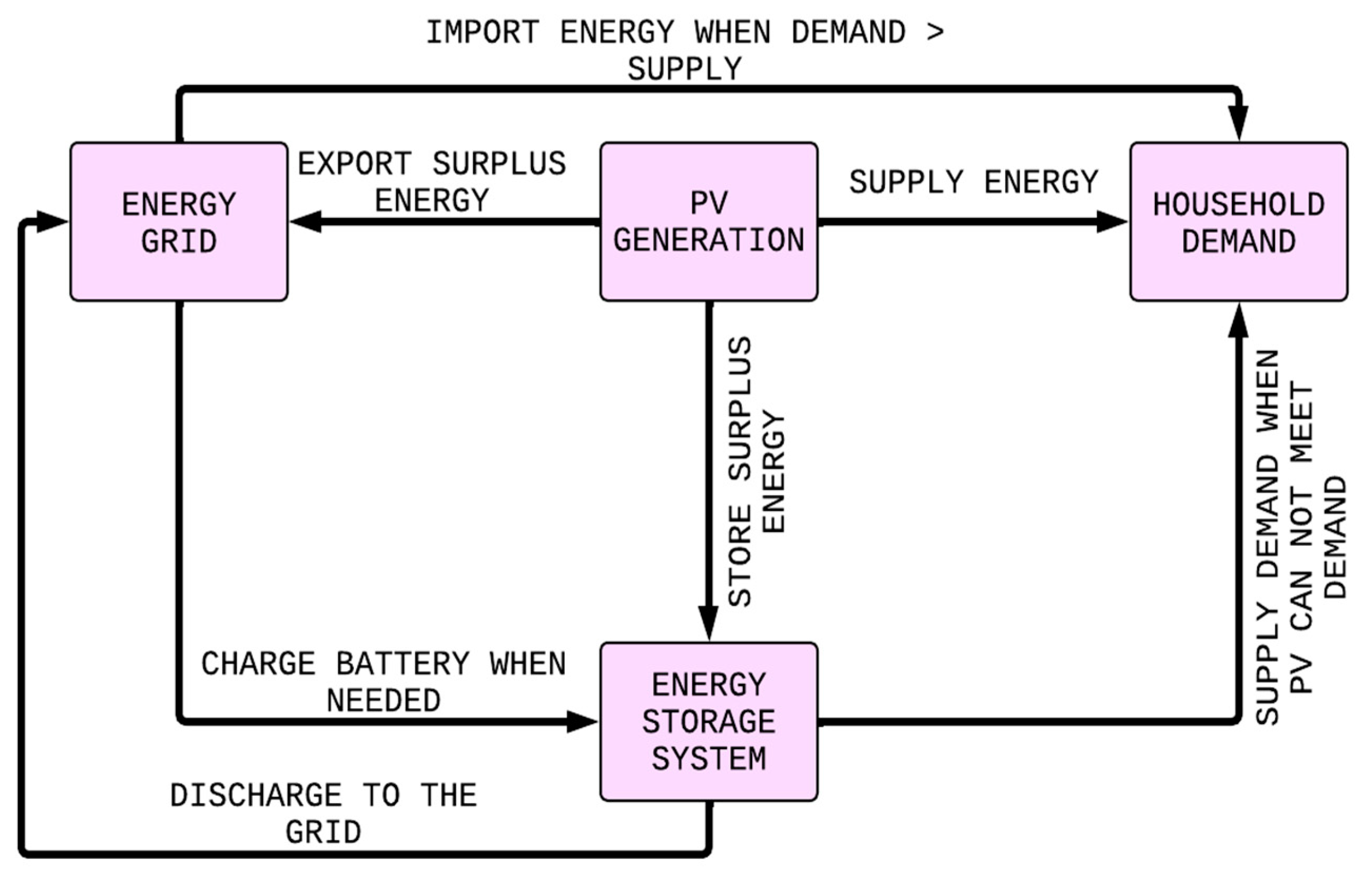Figure 1 illustrates the energy flow in the proposed system, integrating PV generation, ESS, and grid interaction. PV supplies energy to household demand, with surplus stored in the ESS or exported to the grid. The ESS supplies energy during PV shortfalls and exports to the grid when necessary, ensuring efficient energy management.

This article makes three primary contributions:

• A comparative RL and FLC performance analysis across varying SOC levels.
• Insights into trade-offs between profitability, battery health, and system adaptability.
• Practical guidelines for applying control strategies in innovative residential systems.

This study compares RL and FLC in managing ESS SOC within residential energy systems. It evaluates their effectiveness in reducing energy costs, enhancing system adaptability, and responding to real-time fluctuations in energy supply and demand. Additionally, the study investigates how RL can support cost-based sizing and energy management frameworks by addressing residential energy systems’ dynamic and uncertain nature. The findings from this evaluation are expected to inform the development of advanced energy management strategies applicable to residential systems and standalone microgrids, emphasizing optimal resource allocation and operational planning under varying conditions.

2. Materials and Methods

This study compares reinforcement learning, an unsupervised learning approach, and fuzzy logic control, a supervised rule-based technique, for managing the state of charge in energy storage systems. The methodology evaluates the controllers’ ability to optimize energy costs, maintain SOC stability, and minimize battery cycling under varying operational conditions. This section describes the simulation framework, controller designs, evaluation metrics, and statistical analysis to be done.

2.1. System Description

The residential energy system consists of a 3 kW monocrystalline silicon PV array with an inverter efficiency of 95%, a 40 kWh lithium iron phosphate (LiFePO₄) battery with a round-trip efficiency of 90% and a maximum charge/discharge power of 5 kWh, and a grid connection allowing a maximum import/export power of 5 kW. The first layer, illustrated in Figure 2, manages energy distribution by prioritizing PV-generated electricity for household consumption. Surplus energy is stored in the battery, which has a total capacity of 40 kWh and a charge/discharge power limit of 5 kWh, while excess power can be exported to the grid. When demand exceeds generation, the system draws power from the battery or the grid, depending on real-time availability and pricing

The residential load considered in this study follows a typical weekday winter consumption pattern, with an average daily energy demand of 20 kWh and a peak power requirement of 2 kWh. The electricity pricing structure is based on Jordan’s Time-of-Use (TOU) tariff system, as detailed in Section 2.2.1.

This strategy prioritizes solar PV energy and utilizing stored energy in the ESS to meet household demand. The grid is a backup energy source and a repository for surplus energy.

The ESS can import energy from the grid when required or export surplus energy back to the grid. The energy exchange between the ESS and the grid is governed by a second layer that individually employs RL and FLC strategies. The ESS has a storage capacity of 40,000 Wh and is designed to handle a maximum charging or discharging rate of ±5000 W, ensuring alignment with practical constraints in residential energy applications.

The system replicates real-world conditions by incorporating stochastic demand variations, PV fluctuations, and dynamic electricity pricing. This framework provides an adequate basis for evaluating the adaptability and performance of RL and FLC controllers.

2.2. Simulation Framework

The simulation was developed in MATLAB R2024b Simulink, covering 24 h divided into minute-level time steps for detailed analysis. Ten initial SOC scenarios were tested, starting at 0% and increasing in increments of approximately 11.11% up to 100%. These scenarios were evaluated under four distinct cases, as summarized in

Table 1. Simulation test cases for evaluating RL and FLC controllers under varying SOC levels, pricing signals, and demand profiles.

Case	Price Signal	Demand Profile	Details
Case 1	Randomly generated	Randomly generated	Represents dynamic pricing and demand
Case 2	Fixed price (0.12)	Randomly generated	Evaluate performance under higher fixed prices
Case 3	Fixed price (0.08)	Randomly generated	Evaluate performance under lower fixed prices
Case 4	Randomly generated	None	Simulates no household energy demand

, to capture a wide range of operating conditions.

To account for variability in household energy consumption, additional simulations were conducted to represent weekend demand patterns. This extension captures differences in energy usage trends across different days, allowing a more comprehensive evaluation of the control strategies. The impact of weekend consumption fluctuations on charge/discharge cycles and energy trading decisions is analyzed to provide further insights into the adaptability of the proposed approach.

A synthetic demand profile based on widely accepted residential consumption patterns has been used to ensure realistic daily energy trends. The electricity price profile follows Jordan’s Time-of-Use tariff structure, ensuring applicability to real-world pricing conditions. While measured household energy data has not been incorporated in this study, future research will validate the model using real consumption profiles to further assess its robustness under practical operating conditions.

2.2.1. Energy Flow Analysis

To enhance the understanding of how energy is managed within the system, this section provides an analysis of the energy flow dynamics, including the distribution of generated energy, storage behavior, and grid interactions. The energy flow analysis evaluates the system’s ability to balance supply and demand under varying conditions.

The system operation is based on the demand profile, electricity price structure, and photovoltaic (PV) generation characteristics, as described in previous sections. The control strategy is tested under different initial state of charge (SOC) conditions to assess its performance across varying storage levels.

The analysis reveals that when the SOC exceeds 40%, the system operates without relying on grid energy. In these cases, all available PV energy is fully utilized for local consumption, with no surplus exported to the grid. This behavior demonstrates that under moderate to high SOC conditions, the system maintains self-sufficiency without requiring electricity imports.

The energy demand coverage from different sources is illustrated in Figure 3, which presents the contributions of PV generation, battery storage, and the grid in supplying residential demand over a 24 h period. The figure shows the following:

• Battery to Home: The power supplied from the battery storage system to the home, which is discharged during peak demand periods and when PV generation is insufficient.
• PV to Home: The direct utilization of PV-generated power for household consumption, where higher PV contributions are observed during daylight hours.
• Grid to Home: The power imported from the grid, which remains at zero throughout the day when the initial SOC is above 40%, confirming that the system operates independently of external energy sources.

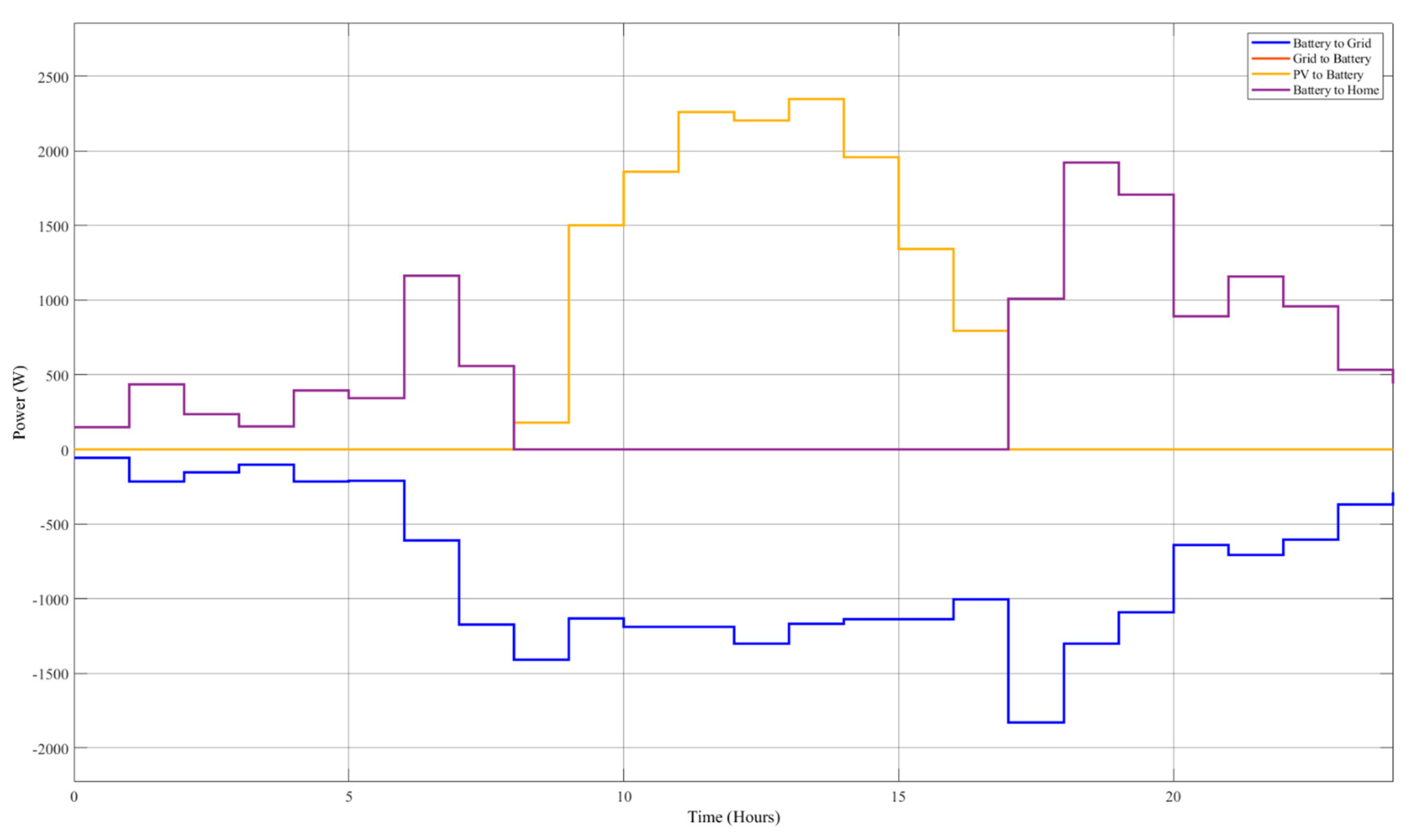
The battery energy flow balance is depicted in Figure 4, illustrating energy exchanges between the battery, grid, and PV system. The following energy flows are analyzed:

• Battery to Grid: Energy discharged from the battery and exported to the grid when excess energy is available.
• Grid to Battery: Energy imported from the grid to charge the battery, which remains minimal, indicating a high reliance on PV generation for charging.
• PV to Battery: The energy directly stored in the battery from PV generation, with charging peaking at midday when solar production is highest.
• Battery to Home: The energy discharged from the battery to supply household load, with negative values indicating discharge during periods of high demand.

These energy flow diagrams highlight the system’s ability to optimize self-consumption by storing excess PV energy during the day and discharging it when needed, effectively reducing reliance on grid electricity. The results confirm that the system dynamically adjusts energy distribution based on available storage capacity, ensuring efficient energy management under different SOC conditions.

2.2.2. Demand and Generation Profiles

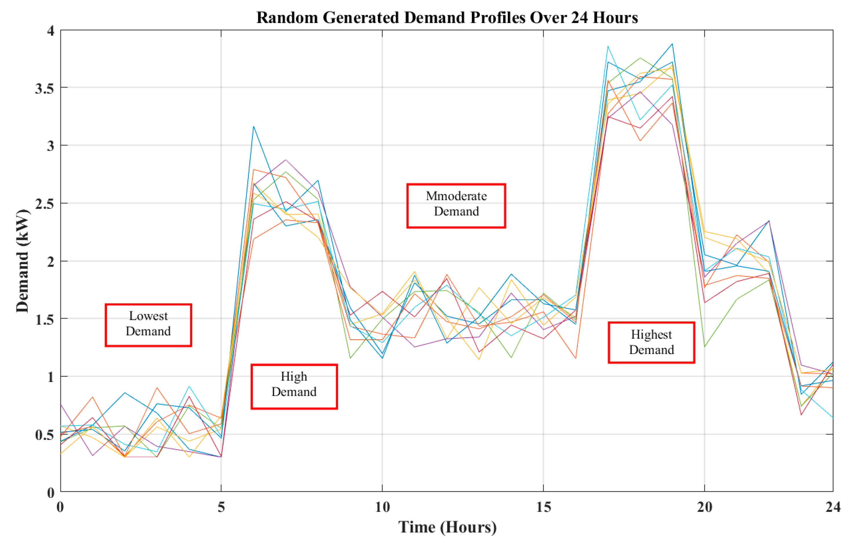
Household energy demand was modeled using stochastic methods to generate time-dependent profiles, reflecting variations typical of residential energy usage. Figure 5 illustrates randomized household demand profiles over one day, highlighting variations between low, high, and peak demand times.

The random demand profiles were generated over 24 h to simulate household energy consumption. These profiles demonstrate significant variability, with the lowest demand occurring during late-night hours and the highest demand during peak periods, such as morning and evening. High-demand peaks are critical in evaluating the system’s performance under stress conditions, while low-demand periods test the system’s efficiency in storing surplus energy. This variability ensures the robustness of the analysis by reflecting realistic consumption patterns and enabling a comprehensive evaluation of the controllers’ adaptability.

2.2.3. Electricity Pricing

The electricity pricing model used in this study follows Jordan’s official residential tariff structure as of June 2024 [34]. This tiered pricing system is designed to encourage energy conservation and follows these rates:

• 1–300 kWh/month: 5 piasters per kWh
• 301–600 kWh/month: 10 piasters per kWh
• Above 600 kWh/month: 20 piasters per kWh

(1 piaster = 0.01 JOD; 1 JOD ≈ 1.41 USD)

The machine learning models (RL and FLC) were tested under this pricing model to evaluate their ability to optimize energy consumption while adapting to cost fluctuations. The pricing structure follows a real-world demand pattern, where peak demand typically results in higher electricity costs.

Additionally, seasonal variations were considered in the study:

• Summer (June–August): Peak demand occurs in the afternoon (2 PM–3 PM) due to air conditioning use.
• Winter (December–February): Peak demand shifts to the evening (5 PM–6 PM) due to heating needs.
• Weekday vs. Weekend Consumption: Electricity demand is generally higher from Sunday to Thursday, with Fridays exhibiting the lowest consumption due to social and religious activities.

The 10 random demand profiles illustrated in different colors in Figure 5 are closely linked to dynamic pricing profiles in Figure 6, where electricity prices fluctuate based on demand, solar energy generation, and stored energy usage. High electricity prices typically align with peak demand periods, such as the morning, when solar energy availability is limited, necessitating greater reliance on grid energy. By the evening period (18:00–21:00), despite higher demand, prices are lower than at the peak due to the contribution of remaining sunshine hours and energy stored in the ESS. Lower prices are observed during late-night hours, corresponding to minimal demand.

This interplay between demand, pricing, and renewable energy highlights how energy management strategies adapt to dynamic market conditions. By incorporating these interdependent factors, the evaluation framework rigorously assesses the performance of RL and FLC controllers in optimizing energy usage and minimizing costs under realistic conditions.

As shown in Figure 5, 10 random dynamic electricity prices ranged from 0.03 to 0.2 USD/kWh were generated, representing peak and off-peak periods. These price variations added complexity to the energy management problem, requiring the controllers to make economically optimized decisions.

Simulation outputs, including SOC, total cost (positive = gain, negative = loss), and battery usage, were recorded for a detailed performance evaluation at each time step. These high-resolution data enabled the identification of trends and variations in controller behavior.

2.3. Controller Design

This study compares RL and FLC in residential energy management, focusing on decision-making strategies based on price fluctuations and battery SOC. The FLC was designed without household demand input to ensure a direct comparison with RL in optimizing energy trading.

While household demand can influence energy decisions, this study isolates price-driven behavior to evaluate the core strengths of each approach. The FLC follows predefined rules for immediate corrective actions, ensuring rapid SOC recovery, while RL learns optimal long-term strategies by adapting to price variations. This distinction highlights the trade-off between structured rule-based control and adaptive decision-making.

2.3.1. RL Controller

The RL controller utilized the PPO algorithm, which was designed for continuous control applications. This algorithm develops a stochastic policy while incorporating a value function critic to evaluate returns. It operates by alternating between collecting environmental interaction data and applying stochastic gradient descent to a clipped surrogate objective. This approach enhances stability by limiting the extent of policy adjustments during each update. The RL controller dynamically modifies charging and discharging rates to optimize energy exchange between the ESS and the grid.

The RL agent observed six variables to understand the system’s operational conditions (State Space):

• Total Demand [kWh]: The overall energy consumption.
• PV Energy [kWh]: Energy generated by the photovoltaic system.
• Battery SOC [%]: Current battery state of charge percentage.
• Grid Injection [kWh]: Energy exported to the grid.
• Grid Withdrawal [kWh]: Energy imported from the grid.
• Dynamic Price Signal [USD/kWh]: Electricity pricing, including randomness for real-world variability.

The RL agent was trained offline on a Lenovo system with an Intel Core i7 processor (Intel Corporation, Santa Clara, CA, USA) and 16 GB RAM, requiring 4–6 h for 5000 training episodes. However, once deployed, the trained model executes real-time energy management decisions within milliseconds, making it feasible for embedded execution in inverters, BMS, or external controllers.

The controller’s output (Action Space) was a continuous variable within [−5000, 5000], representing the battery’s charging or discharging rate in watts. Positive values indicate charging, while negative values represent discharging.

The reward function was designed to achieve the following:

• Maximize profit.
• Discourage frequent cycling, which can degrade battery health.

The mathematical formulation is as follows:

$$R=\left(C_{total }-\lambda \cdot \left|B_{usage}\right|\right)$$

(1)

where

• $C_{total}$: Energy cost based on grid usage and pricing.
• λ: Penalty weight for battery usage, considering the battery capacity this term is empirically tuned during training.
• B_usage: Represents the absolute value of the battery’s energy usage during charging or discharging.

2.3.2. Actor–Critic Network Architecture in PPO

The network architecture in PPO consists of two main networks: the actor network and the critic network, each with their respective layers and connections. Both networks share input but differ in their roles (action generation vs. value estimation).

Networks’ key features:

• Actor network: Processes the observed state (6D state input) from the environment through two rectified linear unit (ReLU)-activated hidden layers, which allows neural networks to model complex, non-linear relationships, representing the controller’s decision. Additionally, it outputs a continuous action (±5000 Wh) via tanh activation, which is ideal for generative model scenarios.
• Critic network: Processes the observed state (6D state input) and the reward value; then, it evaluates the quality of actions using two ReLU-activated hidden layers, and finally outputs a scalar Q-value (linear activation).

During the training process, the PPO agent acts as follows:

• Computes a probability distribution over the available actions and then stochastically samples actions according to these probabilities.
• Executes the actor’s action in the environment and uses the critic network to predict the Q-value for policy updates.
• Gathers experience by applying the current policy in the environment for multiple time steps and afterwards performs several mini-batch updates on the actor and critic networks across multiple epochs.
• Furthermore, the learning process was stabilized by clipping policy updates, which enables multiple epochs of updates on the same batch of data without divergence, limiting the magnitude of changes to prevent instability. The learning rate was set to 10⁻⁴ to balance exploration (trying new actions) and exploitation (refining known good actions), and the discount factor ${\rm Y}$ = 0.99 ensured a balance between immediate and future rewards. Since PPO uses mini-batch updates, batch size was fixed at 64, optimising the trade-off between computational efficiency and learning performance.

2.3.3. RL Training Convergence Analysis

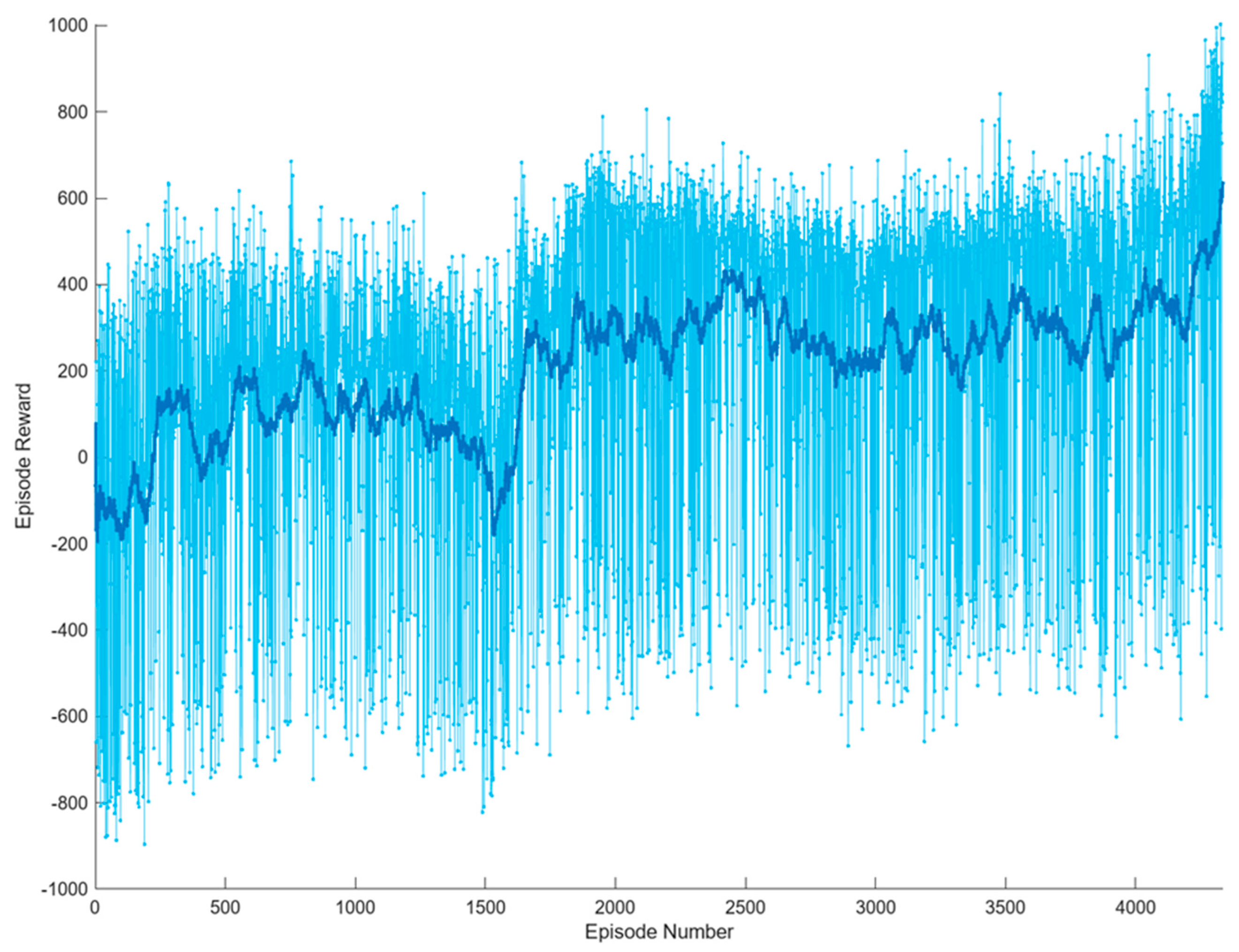
The convergence behavior of the RL agent was analyzed to ensure stable training and optimal performance. Figure 7 presents the episode reward (light blue) and the average reward (deep blue) progression over training iterations, illustrating the improvement in the agent’s decision-making.

The training process exhibited the following learning phases:

• Early Training Phase (Episodes 1–100): The agent initially favored charging the battery from the grid due to a lack of learned policy. The episode reward showed high variance, reflecting random exploration of possible actions.
• Exploration and Policy Refinement (Episodes 100–1500): The agent began experimenting with discharging during peak price periods, learning that energy arbitrage strategies could improve rewards.
• Stabilization and Optimization (Episodes 1500–3500): The reward curve stabilized, demonstrating that the policy was converging toward an optimal energy management strategy.
• Final Policy Convergence (Episodes 3500+): The fluctuations in episode reward decreased, indicating that the RL model had effectively learned to optimize energy trading decisions based on dynamic pricing and battery usage constraints.

To ensure stable training and efficient learning,

Table 2. PPO hyper-parameters used for RL training, optimized for stable learning and efficient policy convergence.

Hyper-Parameter	Value	Purpose
Learning Rate (Actor and Critic)	1.00 × 10−4	Ensures stable gradient updates
Discount Factor	0.99	Encourages long-term optimization
GAE Factor	0.95	Reduces variance in advantage estimation
Clip Factor	0.3	Limits large updates to the policy
Entropy Loss Weight	0.1	Encourages exploration
Mini-Batch Size	128	Controls policy update stability
Number of Epochs per Update	5	Optimizes policy updates efficiently

shows fine-tuned key hyper-parameters of the PPO algorithm as follow:

2.3.4. FLC

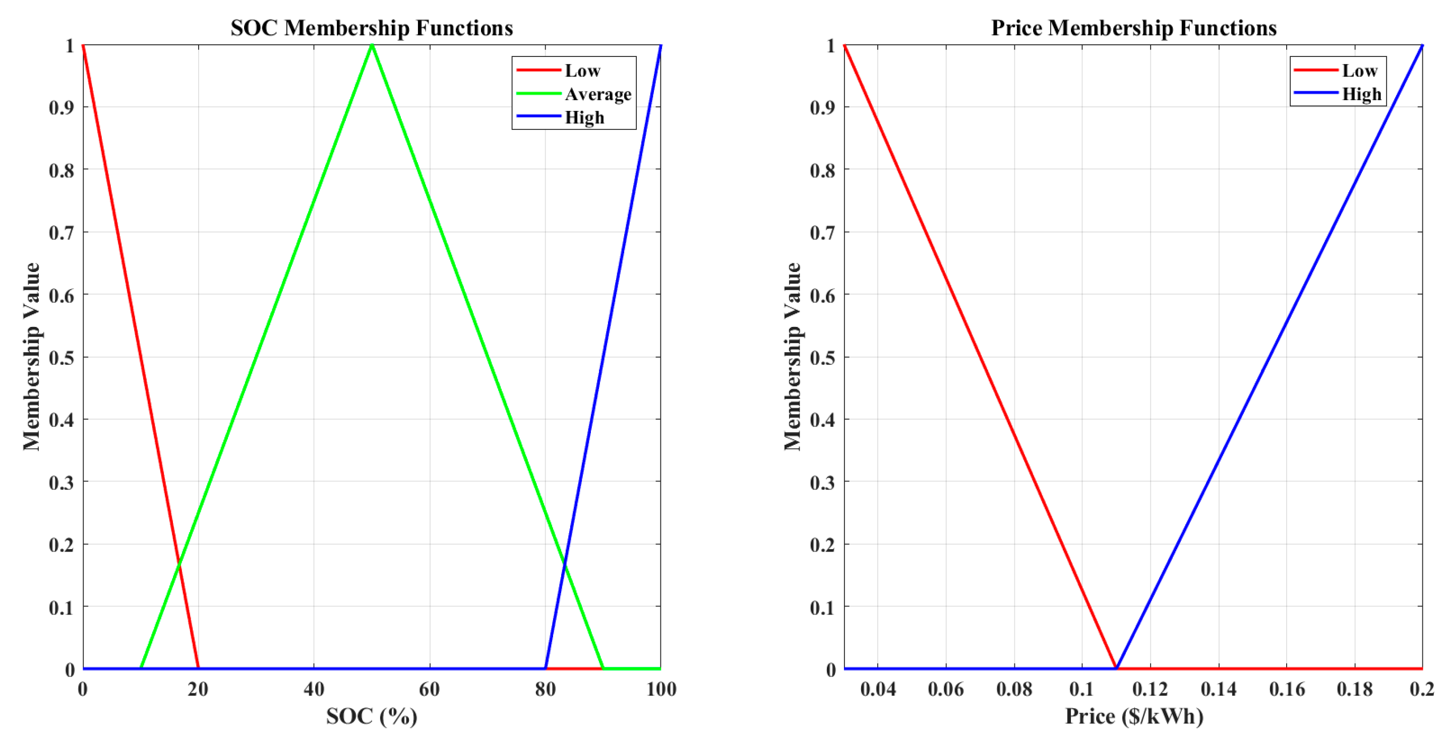
The FLC used predefined linguistic rules to manage SOC based on two inputs: SOC and electricity price. SOC was categorized into three levels—low (<20%), average (20–80%), and high (>80%)—using triangular membership functions (suitable to adjust charging/discharging output using SOC membership value). Electricity prices were categorized into low and high using triangular membership functions (suitable to adjust charging/discharging output using price membership value) and a 0.11 threshold price between low and high prices, as shown in Figure 8 below.

The FLC rules in this study were intentionally designed to prioritize immediate cost savings and fast battery recovery at low SOC levels. This approach ensures rapid responsiveness but lacks adaptability to changing market conditions. While FLC is computationally efficient and effective in predictable energy environments, its reliance on fixed rules makes it less suitable for optimizing long-term energy costs. This distinction allows a clear comparison with RL, which dynamically learns from price and demand variations to achieve adaptive optimization over time.

Six rules governed the FLC decision-making process summarized as follows:

• If SOC is low and the price is low, then maximize charging.
• If SOC and price are high, then maximize discharging.
• Other rules ensured a balance between charging, discharging, and grid dependency.

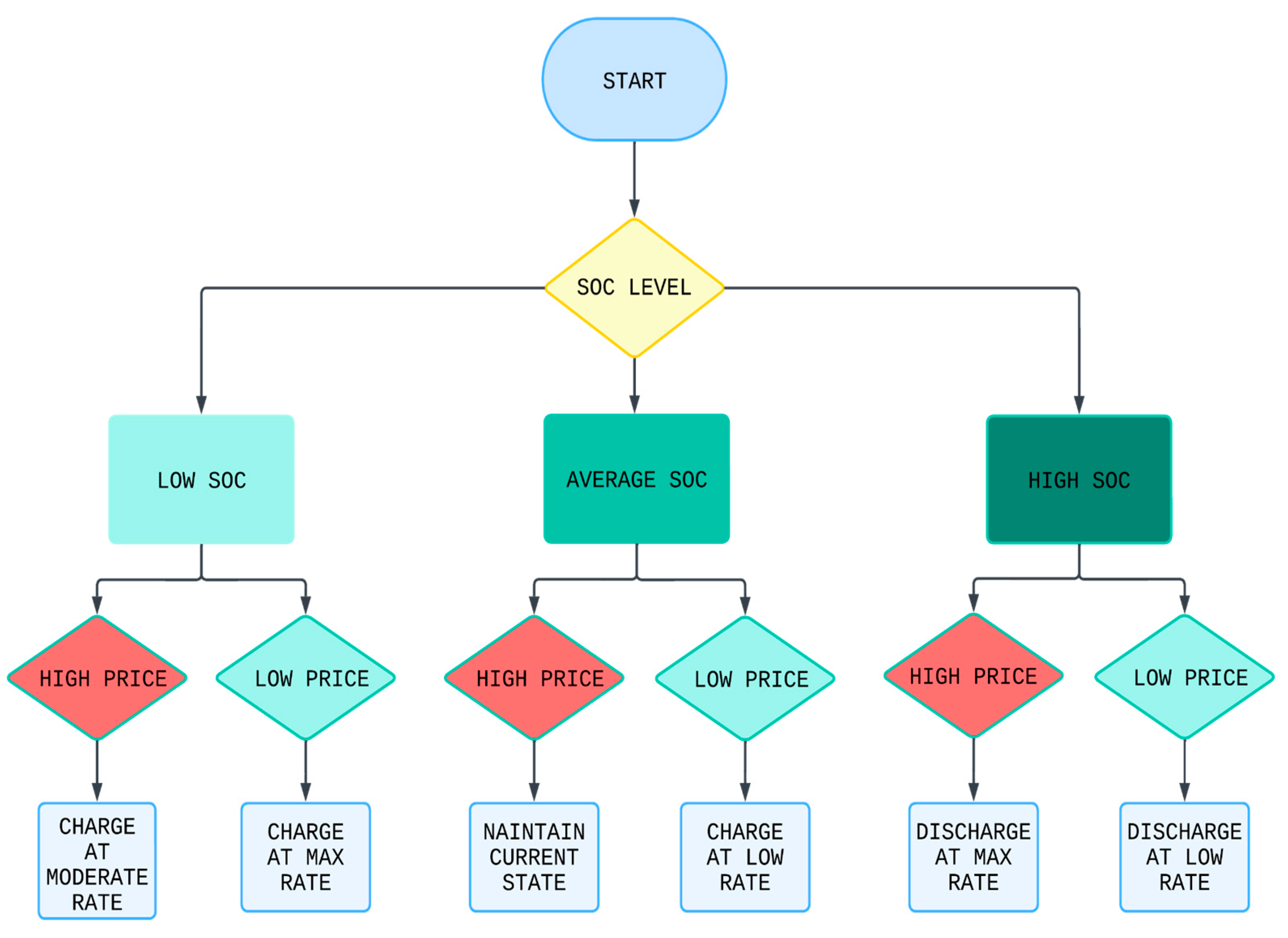
The defuzzification process translated linguistic outputs into actionable charging or discharging rates, ensuring smooth transitions between states. As illustrated in Figure 9, the FLC decision-making process is governed by predefined fuzzy rules. The inputs SOC and electricity price are processed using membership functions, and the defuzzified output determines the charging or discharging rates.

The charging/discharging rate ($\mathrm{R}$) is computed as a function of the membership values $\mathrm{v}$ as follows:

• Moderate charging rate ${\mathrm{R}}_{\mathrm{m}}$

  $${\mathrm{R}}_{\mathrm{m}}=\mathsf{\alpha }\cdot {\mathrm{v}}_{\mathrm{Low} \mathrm{Price}}\left(\mathrm{P}\right)\cdot {\mathrm{v}}_{\mathrm{Low} \mathrm{SOC}}\left(\mathrm{SOC}\right)$$

  (2)

  where
  • $\mathsf{\alpha }$ is a scaling factor for moderate charging.
• Low charging rate ${\mathrm{R}}_{\mathrm{l}}$

  $${\mathrm{R}}_{\mathrm{l}}=\mathsf{\beta }\cdot {\mathrm{v}}_{\mathrm{Low} \mathrm{Price}}\mathrm{L}\left(\mathrm{P}\right)\cdot {\mathrm{v}}_{\mathrm{AVG} \mathrm{SOC}}\left(\mathrm{SOC}\right)$$

  (3)

  where
  • $\mathsf{\beta }$ is a scaling factor for low charging.
• Moderate discharging rate ${\mathrm{R}}_{\mathrm{md}}$

  $${\mathrm{R}}_{\mathrm{md}}=-\mathsf{\gamma }\cdot {\mathrm{v}}_{\mathrm{High} \mathrm{Price}}\mathrm{L}\left(\mathrm{P}\right)\cdot {\mathrm{v}}_{\mathrm{High} \mathrm{SOC}}\left(\mathrm{SOC}\right)$$

  (4)

  where
  • $\mathsf{\gamma }$ is a scaling factor for moderate discharging.
• Low discharging rate ${\mathrm{R}}_{\mathrm{ld}}$

  $${\mathrm{R}}_{\mathrm{ld}}=-\mathsf{\delta }\cdot {\mathrm{v}}_{\mathrm{High} \mathrm{Price}}\mathrm{L}\left(\mathrm{P}\right)\cdot {\mathrm{v}}_{\mathrm{Avg} \mathrm{SOC}}\left(\mathrm{SOC}\right)$$

  (5)

  where
  • $\mathsf{\delta }$ is a scaling factor for low discharging.
• Final output rate R

  $$\mathrm{R}={ \mathrm{R}}_{\mathrm{m}}+{ \mathrm{R}}_{\mathrm{l}}+{ \mathrm{R}}_{\mathrm{md}}+{ \mathrm{R}}_{\mathrm{ld}}$$

  (6)

2.3.5. Real-World Implementation Feasibility

The proposed RL and FLC controllers can be deployed in real-world smart home energy management through different integration strategies. One approach involves embedding the RL model within smart inverter microcontrollers, enabling direct charge/discharge control based on SOC levels and electricity pricing. Another approach is through battery management systems (BMSs), where RL optimizes charging strategies while considering battery longevity and dynamic pricing.

Additionally, home energy management systems (HEMSs) can incorporate these controllers as an external computing unit (e.g., Raspberry Pi or industrial microcontroller) that communicates with system components. These methods rely on standard communication protocols such as Modbus, CAN bus, and MQTT, ensuring compatibility with commercially available inverters and storage systems.

The feasibility of these approaches will be discussed in future work, with emphasis on real-world testing and validation under practical operational conditions.

2.4. Performance Evaluation

The 24 h simulation framework provides a relevant benchmark for evaluating short-term energy trading decisions. Daily cycles in electricity prices, demand fluctuations, and PV generation establish predictable patterns, making a single-day simulation an effective testbed for assessing system performance. Additionally, the reinforcement learning policy is not constrained by a fixed time horizon and can generalize beyond the simulated period, making it applicable to extended operational scenarios.

• Total cost (${\mathrm{C}}_{\mathrm{total}}$): This metric quantifies the economic cost of grid energy usage:

  $${\mathrm{C}}_{\mathrm{total} }={{\displaystyle \int }}_0^{\mathrm{T}}{\mathrm{P}}_{\mathrm{grid}}\left(\mathrm{t}\right)\cdot \mathrm{Price}\left(\mathrm{t}\right)\mathrm{dt}$$

  (7)

  where ${\mathrm{P}}_{\mathrm{grid}}\left(\mathrm{t}\right)$ represents grid energy at time $\mathrm{t}$, and $\mathrm{Price}\left(\mathrm{t}\right)$ is the dynamic electricity price.
• SOC stability (${\mathrm{S}}_{\mathrm{stability}}$): measures the deviation from the target range:

  $${\mathrm{S}}_{\mathrm{stability}}={\displaystyle \frac{1}{\mathrm{T}}}{{\displaystyle \int }}_0^{\mathrm{T}}\left|\mathrm{SOC}\left(\mathrm{t}\right)-{\mathrm{SOC}}_{\mathrm{target}}\right|\mathrm{dt}$$

  (8)

  where ${\mathrm{SOC}}_{\mathrm{target}}$ is the midpoint of the operational range (50%).
  SOC(t): State of charge at a specific time.
  $\mathrm{T}$: Total simulation duration (24 h).
• Battery usage (${\mathrm{B}}_{\mathrm{usage}}$): measures battery usage and evaluates the battery life cycle:

  $${\mathrm{B}}_{\mathrm{usage} }={{\displaystyle \int }}_0^{\mathrm{T}}{\mathrm{P}}_{\mathrm{battery}}\left(\mathrm{t}\right)\mathrm{dt}$$

  (9)

  where ${\mathrm{P}}_{\mathrm{battery}}\left(\mathrm{t}\right)$: The instantaneous energy supplied or absorbed by the battery at time $\mathrm{t}$ (in watts)
• Unified scoring function: The scoring function integrates all metrics:

  $$\mathrm{Score} ={\displaystyle \frac{\mathsf{\alpha }}{\mathsf{\beta }\cdot \left|{\mathrm{C}}_{\mathrm{total}}\right|+{\mathrm{S}}_{\mathrm{stability}}+{\mathrm{B}}_{\mathrm{usage} }}}$$

  (10)

  Here, $\mathsf{\alpha }$ and $\mathsf{\beta }$ are weights to prioritise cost efficiency, stability, or battery usage.

Equation (10) was designed to provide a fair assessment of controller performance by balancing cost minimization, SOC stability, and battery usage efficiency. To prevent any single factor from disproportionately influencing the score, each term was normalized before inclusion. The weight factors were initially selected based on domain knowledge and further refined through sensitivity analysis across different energy price and demand scenarios to ensure consistency in performance evaluation.

The methodology outlined provides a clear and replicable framework for assessing RL and FLC controllers under realistic residential energy conditions. The simulation settings ensure a comprehensive evaluation, while the performance metrics and scoring function provide an objective comparison.

The following section, Section 3, presents the findings, highlighting the performance of RL and FLC under varying SOC conditions. These insights contribute to developing effective energy management strategies

3. Results

This section has been restructured to present the findings in a clear and logical order. The comparative performance of RL and FLC algorithms was evaluated across multiple SOC levels, ranging from 0% to 100%, focusing on SOC evolution, total cost, and battery usage. The analysis follows a structured sequence: SOC evolution dynamic trends, total cost dynamic behavior, battery usage dynamic patterns, and unique correlations with generalized implications. This arrangement ensures a systematic presentation of findings, highlighting distinct patterns and correlations that provide deeper insights into the strengths and limitations of both algorithms.

3.1. SOC Evolution Dynamic Trends

The progression of SOC over time demonstrates clear algorithmic differences. FLC consistently achieved faster SOC replenishment at each initial SOC level. This rapid increase can be attributed to the fuzzy control strategy’s ability to prioritize energy recovery. Conversely, RL exhibited a more gradual SOC progression, likely due to its policy-learning approach optimizing for long-term benefits rather than immediate gains.

At lower SOC levels (e.g., 0% to 33%), the disparity between FLC and RL was more obvious, with FLC achieving up to 20% higher SOC increments within equivalent time frames. However, as SOC levels approached 100%, both algorithms converged towards similar final states, indicating diminishing returns for FLC’s aggressive strategy.

The progression across all initial SOC levels shown in Figure 10 was applied after calculating the net SOC:

$$\mathrm{Net}\_\mathrm{SOC} =\left|\mathrm{SOC}\left(\mathrm{t}\right)-{\mathrm{SOC}}_{\mathrm{initial}}\right|$$

(11)

SOC Comparison Analysis:

• Dynamic Analysis:
  • RL shows steady, gradual SOC score progression across all levels, as seen in the figure, aligning with the cost-efficiency strategy.
  • FLC displays rapid growth, especially at low SOC levels, prioritizing immediate SOC recovery.
• Generalised Trends:
  • The figure confirms that FLC consistently achieves higher SOC scores than RL, particularly at lower initial SOC levels.
  • The gap narrows as initial SOC increases, which aligns with the described performance.
• Implications:
  • RL’s slower growth reflects its focus on long-term optimization and battery preservation, apparent from its gradual progression in the chart.
  • FLC’s rapid SOC recovery ensures system responsiveness but may come at the cost of higher energy usage, consistent with its steep score increase.

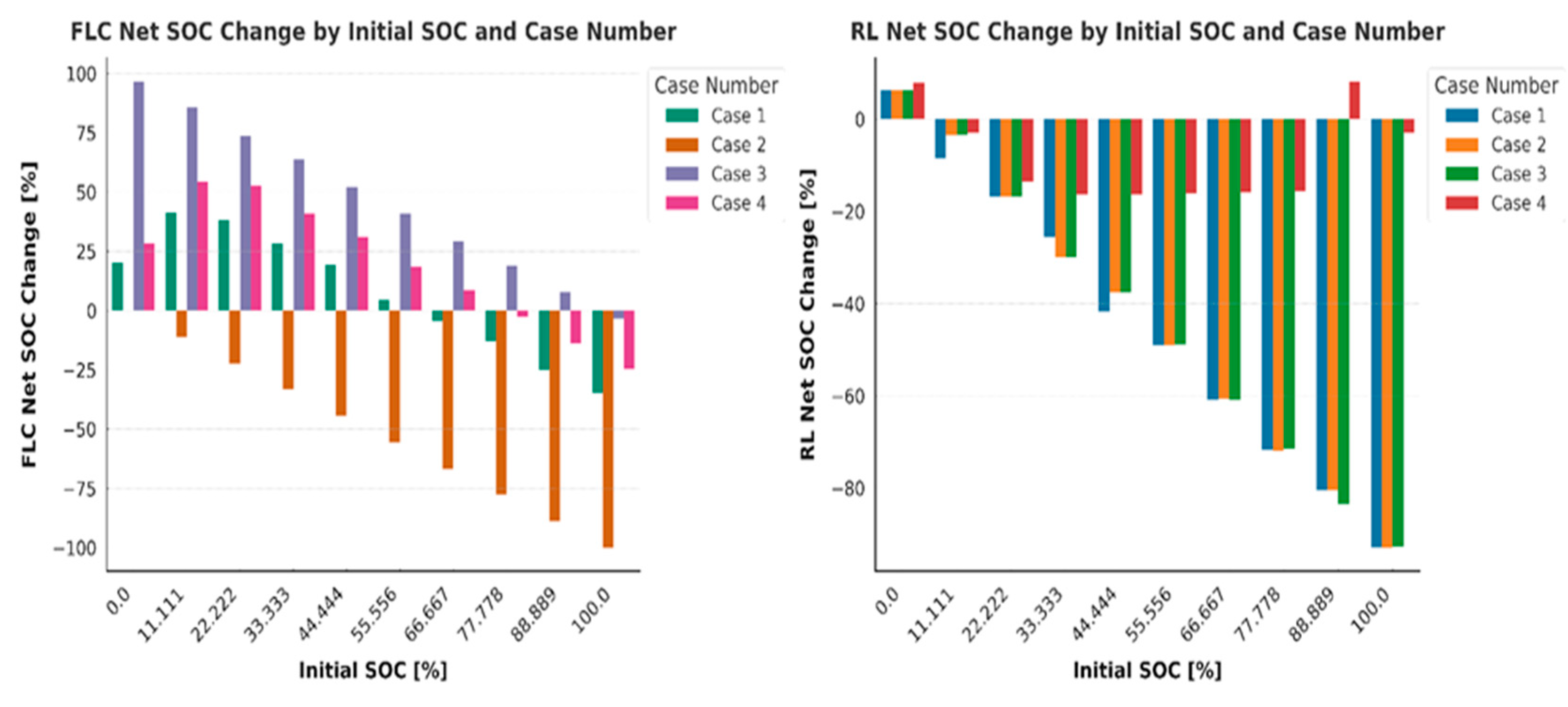
The net SOC change analysis highlights key differences in FLC and RL performance. FLC achieves higher positive SOC changes at low SOC levels in Case 1 (random price and demand) but shows significant negative changes at higher SOC levels, particularly in Cases 2 and 3 (fixed prices) and Case 4 (no demand). This reflects FLC’s aggressive recovery strategy but inefficiency in static or no-demand scenarios, as shown in Figure 11.

RL maintains consistent trends with smaller positive SOC changes at low SOC levels and less extreme negative changes across all cases. Its balanced energy management shows greater stability and cost efficiency, especially in scenarios with static pricing or no demand.

The results highlight the fundamental trade-off between FLC and reinforcement learning-based control. The FLC approach ensures immediate corrective actions to restore battery SOC; however, its predefined rules prevent adaptability to varying electricity prices and load demand patterns. In contrast, RL dynamically adjusts decision-making based on observed market trends, optimizing energy use over an extended period. This difference underscores the limitations of static rule-based control in dynamic energy management scenarios.

3.2. Total Cost Dynamic Behaviour

The total cost (profit/loss) associated with energy management varied significantly between RL and FLC:

• FLC: At lower SOC levels, FLC exhibited profit fluctuations due to its aggressive energy recovery strategy, which prioritized rapid SOC replenishment but incurred higher penalties. For example, at 0% SOC, FLC achieved lower mean profits than RL, reflecting the cost of its prioritization of immediate recovery. This highlights the trade-off between speed and cost efficiency in FLC’s approach.
• RL: This controller demonstrated stable profit trends across all SOC levels, particularly excelling at mid-range SOC levels (33–77%). Its optimized policy effectively balanced profit and SOC progression, maintaining higher profitability in most scenarios.

The trends across SOC levels are illustrated in Figure 12, showing a consistent cost-efficiency advantage for RL in most scenarios.

Profit Comparison:

• Dynamic Analysis:
  • RL demonstrates stable profit progression with fewer fluctuations across all SOC levels.
  • FLC shows significant variability at lower SOC levels, gradually stabilizing as SOC increases.

2.

Generalized Trends:

• At lower SOC levels (e.g., 0% to 33%), RL achieves higher profits than FLC due to its cost-efficient strategy.
• As SOC levels rise above 44%, FLC begins to close the gap but remains below RL in overall profitability.

3.

Implications:

• RL is better suited for scenarios prioritizing cost-efficiency and battery health, particularly at lower SOC levels.
• FLC’s variability reflects its dynamic adaptation and rapid recovery, which is beneficial in maintaining system performance under low SOC conditions.

The profit distribution highlights RL’s consistent performance across all cases and SOC levels, with higher profits at mid-to-high SOC levels, especially in Case 1 (random price and demand). FLC shows high profits at low SOC levels in Case 1 due to aggressive charging over all the 10 different SOC (each colored bar represents a SOC from 0–100, left to right respectively). but performs poorly in Cases 2 and 3 (fixed prices), with significant negative profits at mid and high SOC levels, as shown in Figure 13.

In Case 4 (no demand), RL maintains stable positive profits, reflecting its adaptability, while FLC suffers negative profits at lower SOC levels, improving only slightly at higher SOC levels. RL’s robustness contrasts with FLC’s dependence on dynamic pricing and demand conditions.

The results indicate that RL demonstrated a greater ability to minimize costs under fluctuating price conditions compared to FLC, which was more reactive to immediate energy price variations. Under Jordan’s tiered pricing structure, RL successfully delayed charging to avoid higher electricity costs, leveraging the lower-cost periods for battery recharging. In contrast, FLC prioritized maintaining SOC levels, often leading to charging during high-cost periods, which resulted in higher overall electricity expenses.

3.3. Battery Usage Dynamic Patterns

The analysis of battery usage further underscores the differences in algorithmic behavior; the progression shown in Figure 14 shows the following:

• FLC: Rapid SOC replenishment caused significant spikes in battery usage, especially at lower SOC levels, aligning with its prioritization of immediate SOC gains.
• RL: Maintained consistent and gradual battery usage patterns, reflecting its focus on optimizing costs and preserving battery health.

Battery Usage Comparison Analysis:

• Dynamic Analysis:
  • RL gradually increases battery usage as SOC rises, reflecting its conservative energy management strategy.
  • FLC shows consistently higher battery usage, particularly at lower SOC levels, due to its aggressive charging approach. Battery usage decreases significantly as SOC approaches 100%.
• Generalized Trends:
  • At lower SOC levels, FLC utilizes the battery more extensively, maintaining usage approximately 4–5 times higher than RL.
  • As SOC increases, FLC battery usage declines steadily, converging towards RL’s usage levels near complete SOC (100%).
• Implications:
  • RL’s gradual battery usage aligns with its focus on long-term battery health and cost efficiency.
  • FLC’s high initial usage ensures rapid SOC recovery but may increase wear on the battery, making it less ideal for scenarios prioritizing battery longevity.

The battery usage patterns highlight key differences between FLC and RL, as shown in Figure 15. FLC exhibits high battery usage at low SOC levels in Case 1 (random price and demand), reflecting its aggressive charging strategy. This usage decreases at higher SOC levels and in Cases 2 and 3 (fixed prices), and 4 (no demand), showing reduced reliance on energy recovery.

RL shows consistent and gradual battery usage across all SOC levels and cases. Case 1 results in slightly higher usage due to dynamic conditions, while Cases 2, 3, and 4 show minimal fluctuations, reflecting RL’s focus on stable, long-term optimization.

The analyses in the previous sections focused on SOC progression, cost dynamics, and battery usage patterns, highlighting the operational differences between RL and FLC across varying scenarios. The following section builds on these insights by examining the 24 h patterns, uncovering unique correlations and general trends in controller performance.

3.4. Unique Correlations and Generalised Implications

3.4.1. Model Performance Comparison

The performance of RL and FLC controllers was evaluated through statistical and machine learning models to predict SOC, total cost, and battery usage. Random forest regression (RFR) demonstrated exceptional accuracy in capturing the complex relationships between inputs (time and initial SOC) and outputs, significantly outperforming multiple linear regression (MLR). This section summarizes the findings and discusses their implications for dynamic energy management.

The MLR equations in

Table 3. MLR equations for predicting net SOC, total cost, and battery usage for RL and FLC controllers, showing the influence of time and Initial SOC.

Controller	Output	Equation
RL	Net SOC	$Net\_SOC=19.3946+\left(-2.0028\right)\times Time+0.5905\times Initial\_SOC$
RL	Total Cost	$Total\_Cost=\left(-1310.491\right)+131.5428\times Time+20.6216\times Initial\_SOC$
RL	Battery Usage	$Battery\_Usage=\left(-6808.85\right)+1094.88\times Time+117.73\times Initial\_SOC$
FLC	Net SOC	$Net\_SOC=54.0111+\left(-0.4614\right)\times Time+0.4237\times Initial\_SOC$
FLC	Total Cost	$Total\_Cost=\left(-1741.0056\right)+157.4723\times Time+12.9360\times Initial\_SOC$
FLC	Battery Usage	$Battery\_Usage=12376.48+3733.53\times Time+\left(-285.61\right)\times Initial\_SOC$

and the 3D scatter plots in Figure 16 highlight the distinct strategies of RL and FLC controllers. In terms of the net SOC data, RL exhibits a stable decline over time, with the initial SOC positively influencing retention. The scatter plots confirm this predictable behavior with smooth trends. FLC shows more significant variability, reflecting its focus on immediate SOC recovery rather than consistency.

In total cost comparison data, RL demonstrates gradual increases, indicating controlled cost management, while FLC displays significant fluctuations at lower SOC levels due to its aggressive energy strategies. while in terms of battery usage, RL maintains steady growth, balancing resource use over time. FLC, however, shows high usage at low SOC levels, tapering off at higher levels, prioritizing rapid recovery but with more significant variability.

These results highlight RL’s stability and long-term efficiency, contrasting with FLC’s dynamic but variable performance across all metrics.

3.4.2. Key Insights from the Analysis

The predictive accuracy of MLR and RFR is summarized in

Table 4. MLR and RFR performance comparison.

Controller	Output	MLR R2	RFR R2	Feature Importance (Time, Initial SOC − RFR)
RL	SOC	0.93	0.99999	Time: 42.4%, Initial SOC: 57.6%
RL	Total Cost	0.76	0.99997	Time: 65.2%, Initial SOC: 34.8%
RL	Battery Usage	0.95	0.99997	Time: 71.8%, Initial SOC: 28.2%
FLC	SOC	0.38	0.95168	Time: 49.0%, Initial SOC: 51.0%
FLC	Total Cost	0.77	0.99992	Time: 79.4%, Initial SOC: 20.6%
FLC	Battery Usage	0.98	0.99998	Time: 85.7%, Initial SOC: 14.3%

, which includes R² values and the relative feature importance (for RFR). The feature importance indicates the contribution of the time and the initial SOC to the predictions.

• RL Controller:
  • RFR Accuracy: Achieved nearly perfect predictions for all outputs, with R² values exceeding 0.9999 for SOC, total cost, and battery usage.
  • Feature Importance: Initial SOC played a more significant role in predicting SOC, while time had a greater influence on total cost and battery usage.
  • MLR Performance: MLR achieved reasonable accuracy (R² = 0.93 for SOC, R² = 0.95 for battery usage) but fell short in predicting total cost (R² = 0.76) due to its inability to capture non-linear patterns.
• FLC Controller:
  • RFR Performance: Significantly improved prediction accuracy for total cost (R² = 0.99992) and battery usage (R² = 0.99998), although SOC predictions remained moderate (R² = 0.95168).
  • Feature Importance: Time dominated the total cost and battery usage prediction, reflecting FLC’s reliance on time-dependent operational dynamics.
  • MLR Limitations: MLR struggled to predict SOC accurately (R² = 0.38), indicating its inability to handle non-linear dependencies effectively.

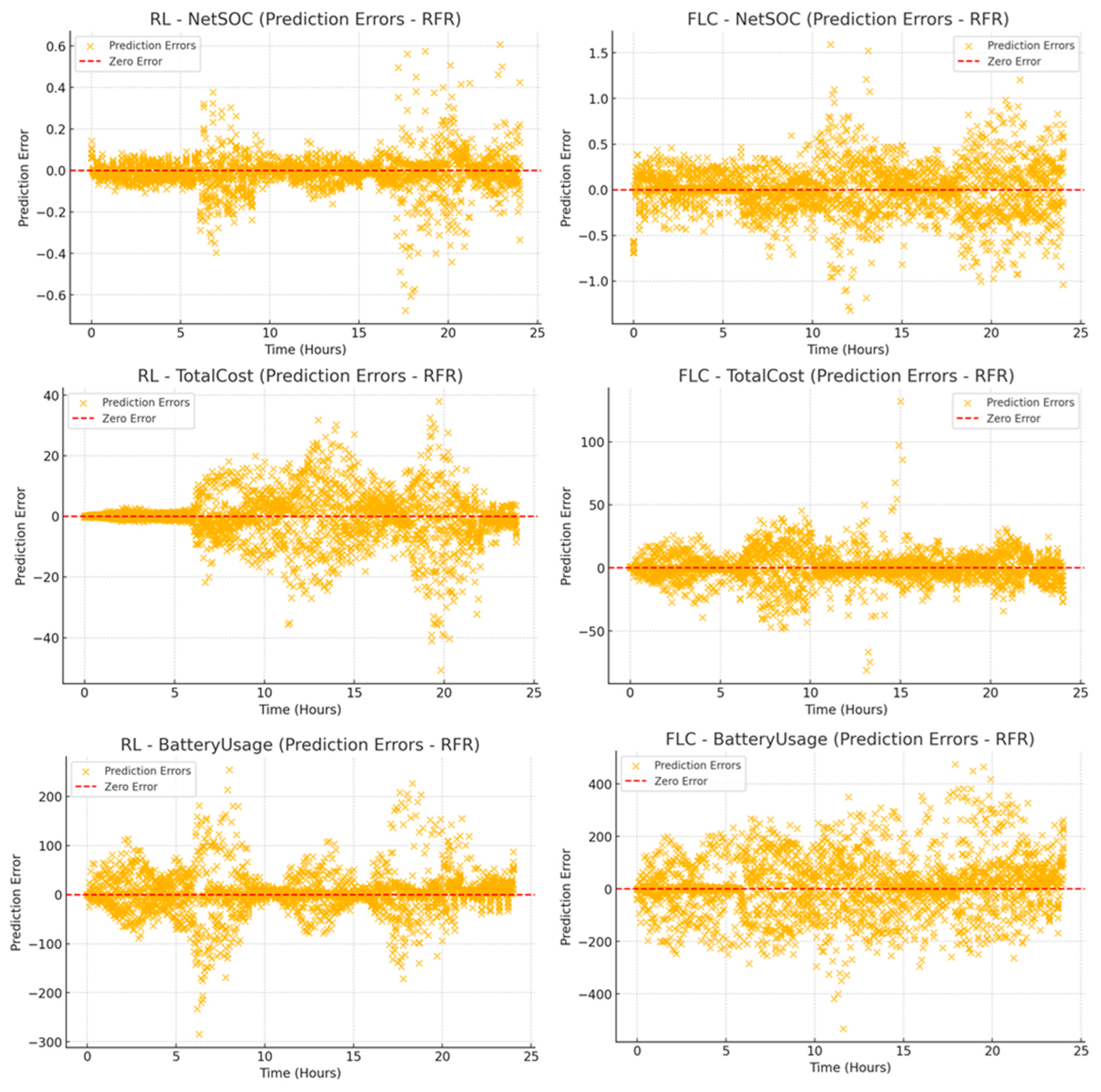
Finally, the prediction error plots in Figure 17 validate the high accuracy of the RFR model, supported by the R² values in Table 4.

For the net SOC data, RL shows tight error distributions (R² = 0.99999), driven by initial SOC (57.6%). FLC, with a slightly lower R² (0.95168), exhibits greater variability due to its dynamic recovery strategies. For the total cost data, RL maintains consistent predictions (R² = 0.99997) with time (65.2%) as the dominant factor. FLC achieves substantial accuracy (R² = 0.99992) but shows more significant error fluctuations, reflecting its time-sensitive cost adjustments (79.4%). For the battery usage data, RL demonstrates stable predictions (R² = 0.99997), with time (71.8%) as the key influence. Despite achieving the highest R² (0.99998), FLC displays significant variability due to its aggressive energy recovery, driven primarily by time (85.7%). RL offers stable and predictable performance, while FLC shows more significant variability despite high prediction accuracy.

4. Conclusions

This study conducted a comparative evaluation of reinforcement learning (RL) and fuzzy logic control (FLC) for managing energy storage in residential systems equipped with photovoltaic (PV) panels, battery-based energy storage systems (ESS), and dynamic or fixed electricity tariffs. The simulations covered minute-level operations over 24 h, exploring diverse starting SOC levels and demand patterns to assess their effectiveness in balancing electricity cost, battery longevity, and operational flexibility under realistic conditions. The key findings are as follows:

• Rapid charging at low SOC levels: FLC could rapidly refill battery charge when SOC was near zero, addressing critical energy shortages. However, this quick response led to significant power draw from external sources, particularly under fixed pricing schemes or low household demand conditions.
• Cost optimization through adaptive learning: RL autonomously developed optimal charging and discharging schedules by learning from evolving data, avoiding unnecessary cycling. This adaptive approach achieved consistent cost reductions across all SOC levels, especially in scenarios with variable electricity tariffs.
• Diverging battery usage patterns: FLC’s emphasis on swift recharging caused pronounced peaks in battery usage, potentially accelerating wear over time. RL adopted a more gradual approach, smoothing energy flows and minimizing abrupt changes, which supported longer battery life.
• Role of initial SOC and pricing models: Each method exhibited unique strengths depending on the initial SOC. FLC was most effective at extremely low SOC levels, whereas RL maintained cost efficiency at moderate to high SOC levels. Dynamic pricing environments further underscored RL’s ability to adapt decisions and minimize costs during high-price periods.
• Hybrid potential for enhanced performance: The findings suggest potential benefits from combining FLC’s quick responsiveness at low SOC with RL’s adaptive, cost-efficient strategies. Such a hybrid approach could enhance economic performance while preserving battery health, particularly in systems subjected to frequent demand or price fluctuations.

This study provides a structured comparison between RL and FLC in residential energy management, highlighting their distinct decision-making strategies. RL continuously adapts to changing conditions, optimizing energy usage over time, while FLC follows predefined rules, ensuring immediate responses but lacking long-term adaptability. This comparison establishes a foundation for evaluating their individual advantages and identifying areas where a combined approach could enhance system performance.

The results demonstrate that RL-based optimization achieves greater cost efficiency and improved energy utilization compared to FLC. By dynamically adjusting decisions based on real-time electricity prices and battery SOC, RL minimizes operational costs while maintaining system stability. Although FLC offers fast responses to changing conditions, its rule-based operation leads to higher cycling rates and increased costs under stable energy demand. The findings suggest that while RL is more effective in long-term optimization, FLC remains beneficial in scenarios requiring immediate corrective actions.

Building on these insights, integrating RL and FLC into a hybrid control strategy could combine the adaptability of RL with the rapid decision-making of FLC. This approach has the potential to enhance energy management by leveraging RL’s ability to learn optimal strategies while maintaining the fast-reacting nature of FLC. Future research should explore this integration and assess its real-world feasibility, ensuring compatibility with existing smart home infrastructures, inverters, and communication protocols.