Abstract
Deep learning has achieved remarkable success in various domains; however, its application to tabular data remains challenging due to the complex nature of feature interactions and patterns. This paper introduces novel neural network architectures that leverage intrinsic periodicity in tabular data to enhance prediction accuracy for regression and classification tasks. We propose FourierNet, which employs a Fourier-based neural encoder to capture periodic feature patterns, and ChebyshevNet, utilizing a Chebyshev-based neural encoder to model non-periodic patterns. Furthermore, we combine these approaches in two architectures: Periodic-Non-Periodic Network (PNPNet) and AutoPNPNet. PNPNet detects periodic and non-periodic features a priori, feeding them into separate branches, while AutoPNPNet automatically selects features through a learned mechanism. The experimental results on a benchmark of 53 datasets demonstrate that our methods outperform the current state-of-the-art deep learning technique on 34 datasets and show interesting properties for explainability.
1. Introduction
Tabular data, characterized by their structured format of rows and columns, is ubiquitous in real-world applications across diverse fields such as finance, healthcare, marketing, and social sciences [1]. They encompass datasets like financial transactions, patient health records, customer demographics, and experimental results. Despite the significant advancements in deep learning (DL) for unstructured data domains like computer vision and natural language processing, its application to tabular data has not witnessed comparable success. Traditional Machine Learning (ML) models, particularly ensemble methods like Gradient Boosting Machines and Random Forests, often outperform DL models on tabular datasets [2]. Several factors contribute to this discrepancy. Tabular data frequently involve heterogeneous feature types, including numerical, categorical, and ordinal variables. The relationships between these features can be complex, involving non-linear interactions and hierarchical dependencies that are challenging for standard neural network architectures to capture effectively [3]. Additionally, tabular data lack the spatial or temporal structure that convolutional and recurrent neural networks exploit in image and sequence data [4].
Recent research efforts have sought to adapt DL models to the peculiarities of tabular data. Approaches like TabNet [5], NODE [6], and DeepGBM [7] have introduced novel architectures, incorporating feature-wise attention mechanisms, differentiable decision trees, and hybrid models combining neural networks with gradient boosting techniques. In particular, FT-Transformer’s transformer-based architecture stands out as the top-performing deep model on an extensive benchmark, thus setting the state of the art (SoA) for DL [2,8].
While these models have achieved some success, there remains a performance gap compared to traditional methods, particularly in capturing intricate feature interactions without extensive feature engineering. An unexplored avenue in this context is the exploitation of intrinsic periodicity within tabular data, while literature reviews claim for specialized deep encoders [9,10]. Periodicity refers to patterns that repeat at regular intervals, and it is a common phenomenon in many real-world datasets [11]. For instance, seasonal trends in sales data, circadian rhythms in biological measurements, and cyclical fluctuations in economic indicators all exhibit periodic behavior. Modeling such patterns can provide significant predictive advantages. We propose leveraging the periodicity inherent in many tabular data datasets to address this gap and to enhance DL models for regression and classification tasks. Our approach is grounded in the observation that many tabular datasets, though lacking explicit temporal or spatial structure, may still embody periodic patterns due to the nature of the data collection process or underlying phenomena.
We introduce novel neural network architectures designed to enhance the modeling of diverse patterns in tabular data. Our approach leverages specialized encoding techniques to capture periodic and non-periodic structures, improving the network’s ability to extract meaningful representations. Building on these foundations, we propose integrated architectures that dynamically adapt to different feature types, optimizing predictive performance without manually categorizing the features as periodic and non-periodic.
One of the key challenges in applying DL to tabular data is the lack of inherent explainability [12], which often makes traditional tree-based models preferable in industrial and scientific applications [13]. We address the challenge of explainability in DL for tabular data with an approach that offers a more intuitive understanding of learned representations while retaining high accuracy. By leveraging novel encoding techniques, our method provides a more transparent representation of data patterns, making DL models more accessible and practical for industrial and scientific applications.
1.1. Contribution
This paper introduces a novel approach to leveraging periodicity in tabular DL by integrating Fourier-based encodings, which effectively capture cyclic patterns in data and enhance predictive performance. In parallel, we address the challenge of modeling non-periodic relationships by incorporating Chebyshev polynomials into a neural encoder. This enables the representation of complex, non-linear dependencies that do not exhibit periodic behavior. We propose two architectures, seamlessly integrating periodic and non-periodic encoders to unify these concepts. These are designed to balance feature representations either manually or automatically, thus broadening their applicability across diverse datasets. To validate the effectiveness of our approach, we conduct extensive empirical evaluations on a benchmark of 53 datasets spanning multiple domains and task types, including regression and classification. Our results demonstrate that the proposed models outperform FT-Transformer, the SoA DL method, on 34 datasets, highlighting their robustness and generalizability (The code related to our experiments is publicly available for ease of reproducibility of the results: https://github.com/matteo-rizzo/periodic-tabular-dl) (accessed on 10 March 2025). Beyond performance gains, our approach significantly enhances model explainability. Fourier encodings provide clear insights into the frequency components of features, while Chebyshev polynomials offer an intuitive representation of complex non-linear interactions. By directly connecting these mathematical properties, our method bridges the gap between DL and explainable ML.
1.2. Structure of the Article
Section 2 reviews the existing literature on DL for tabular data, focusing on recent architectural innovations and methods utilizing Fourier and Chebyshev transformations within neural networks. This section sets the foundation for understanding the advancements introduced by our models. Section 3 presents the design and methodology of FourierNet, ChebyshevNet, Periodic-Non-Periodic Network (PNPNet), and AutoPNPNet. We delve into the mathematical foundations of the Fourier and Chebyshev encoders and describe how these components integrate into the overall network architectures to capture periodicity and non-linearity effectively. Section 4 and Section 5 outline our experimental setup, including dataset selection, baseline models, training protocols, and evaluation metrics. We then present the empirical results in Section 6, showcasing how our models compare to the SoA method in terms of performance. The explainability of the proposed methods is detailed in Section 7. Section 8 provides a detailed discussion where we analyze the effectiveness of our models, explore the impact of incorporating periodicity in tabular data, and consider the advantages of our approach and its potential limitations. We also suggest directions for future research, including extending our models to handle categories with a more context-aware strategy. Finally, Section 9 concludes this paper with a summary of our findings.
2. Related Work
Applying DL to tabular data has been a subject of significant research interest, aiming to replicate the success of DL in unstructured data domains such as computer vision and natural language processing [14]. This section reviews the existing literature on DL architectures tailored to tabular data, the use of Fourier transforms and Chebyshev polynomials in neural networks, and methods for capturing periodicity and non-linearity in data.
2.1. DL Architectures for Tabular Data
Traditional ML models, particularly ensemble methods like Gradient Boosting Machines [15] and Random Forests [16] have historically outperformed DL models on tabular datasets [1]. These models are adept at handling heterogeneous feature types and complex interactions without extensive preprocessing. However, DL offers potential advantages in automatic feature extraction and representation learning. TabNet introduced a sequential attention mechanism that enables the model to focus on the most relevant features at each decision step [5]. By mimicking the decision-making process of gradient boosting, TabNet combines feature selection with explainability, allowing for better handling of tabular data’s unique characteristics. Neural Oblivious Decision Ensemble (NODE) involves an architecture integrating differentiable decision trees into a neural network framework [6]. NODE uses oblivious decision trees, where the same feature and threshold are used across all decision nodes at the same depth, enabling efficient representation learning and scalability. DeepGBM combined the strengths of gradient boosting and deep neural networks by using gradient boosting trees to preprocess the data and generate input features for the neural network [7]. This hybrid approach leverages the powerful feature transformations of gradient boosting while benefiting from the representation learning capabilities of DL. FT-Transformer applied the Transformer architecture to tabular data by utilizing feature tokenization and self-attention mechanisms [8]. By treating each feature as a token, FT-Transformer models the interactions between features through self-attention, capturing linear and non-linear relationships without explicit feature engineering. TabTransformer focused on modelling categorical features in tabular data using Transformer-based embeddings and self-attention [17]. TabTransformer captures dependencies and interactions that traditional one-hot encoding methods might miss by learning contextual embeddings for categorical variables. Despite these advancements, challenges remain in modelling the complex and diverse patterns inherent in tabular data, especially when capturing periodicity and non-linearity without significant manual feature engineering.
2.2. Capturing Periodicity with Fourier Transforms
Periodicity is a common characteristic in various data types, manifesting as repeating patterns over regular intervals. Traditional methods for handling periodicity often involve feature engineering techniques like creating lag features or using domain-specific transformations [18]. Fourier transforms have been employed in neural networks to capture periodic patterns by transforming data into the frequency domain [19]. Fourier features allow models to represent functions with high-frequency components more effectively. Random Fourier Features were introduced to approximate kernel functions computationally and efficiently [20]. By mapping input data into a randomized low-dimensional feature space using sinusoidal functions, these features enable linear models to capture non-linear patterns associated with periodicity. Positional encoding in Transformers utilizes sinusoidal functions to inject sequence information into sequential data models [21]. The sine and cosine functions of varying frequencies enable the model to distinguish between different positions in the input sequence, implicitly capturing periodic relationships. Implicit neural representations with periodic activation functions have been explored to model high-frequency variations in data [22]. Using sinusoidal activation functions, neural networks can represent detailed signals and textures, which is particularly useful in tasks like image generation and reconstruction. However, the application of Fourier-based encoding to general tabular data, which may not have explicit temporal or spatial dimensions, has been limited. Our work extends Fourier transforms to tabular data by designing a Fourier-based neural encoder that captures intrinsic periodic patterns within the features without relying on explicit time or spatial information.
2.3. Modeling Non-Linearity with Chebyshev Polynomials
Non-linear relationships are prevalent in tabular data and challenge models that primarily capture linear interactions. Chebyshev polynomials, a sequence of orthogonal polynomials, are well suited for approximating complex non-linear functions due to their minimax properties and numerical stability [23]. In neural networks, Chebyshev polynomials have been utilized in several contexts. A recent study of SS et al. [24] presents Chebyshev Kolmogorov–Arnold Network, a novel neural network architecture, drawing inspiration from the Kolmogorov–Arnold representation theorem, which leverages the robust approximation abilities of Chebyshev polynomials. This is achieved by employing learnable functions, which are parameterized by Chebyshev polynomials, along the network’s edge. Spectral Graph Convolutional Networks have employed Chebyshev polynomials to define convolutional filters in the spectral domain of graphs [25]. By approximating the graph’s Laplacian eigenvalues, these models perform localized filtering operations without needing explicit eigenvalue decomposition. For function approximation, Chebyshev polynomials have been used to approximate arbitrary functions within neural networks [26]. This approach allows networks to represent functions with rapid variations and non-linearities efficiently. Our Chebyshev-based neural encoder leverages these properties to capture non-periodic, complex, non-linear patterns in tabular data. By transforming input features through Chebyshev polynomials, the encoder enables the neural network to approximate intricate relationships that standard linear or non-linear transformations might not capture effectively.
2.4. Integrated Approaches for Periodic and Non-Periodic Patterns
While Fourier transforms and Chebyshev polynomials individually address periodicity and non-linearity, real-world tabular datasets often contain a mixture of both types of patterns. Integrated approaches are necessary to capture the full spectrum of relationships within the data. Our proposed architectures, PNPNet and AutoPNPNet, combine the strengths of both Fourier and Chebyshev encoders. PNPNet involves an a priori separation of features into periodic and non-periodic categories. This explicit division allows each encoder to specialize in modelling its designated feature type, improving the overall representation learning. AutoPNPNet addresses the limitations of manual feature separation by feeding all features into both encoders. An attention mechanism learns to automatically weigh and select features from each encoder, effectively performing feature selection and combination in a data-driven manner. These architectures draw inspiration from models that incorporate multiple types of feature transformations or multiple branches to capture different aspects of the data [21,27]. By integrating specialized encoders, the models can handle heterogeneous patterns more effectively than architectures that rely on a single transformation method.
2.5. Feature Selection and Automatic Relevance Determination
Feature selection is crucial in modelling tabular data due to the presence of irrelevant or redundant features that can degrade model performance. Neural networks often lack inherent mechanisms for feature selection, leading to research on integrating feature selection into DL models [28]. Attention mechanisms have been widely used to enable models to focus on the most relevant parts of the input [29,30]. In tabular data models, attention can be applied to features, allowing the network to weigh the importance of each feature dynamically. Sparse regularization techniques, such as L1 regularization, encourage sparsity in the model weights, effectively zeroing out less important features [31]. This approach can lead to more interpretable models and reduce overfitting. In a study by Li et al. [32], automatic feature selection networks were proposed to learn feature importance scores during training. These networks can suppress irrelevant features and enhance the representation of significant ones, improving both performance and explainability. TabNet [5], uses a sparse feature mask at each decision step to select important features on an instance-by-instance basis. This mask is trained with information from the previous step. A feature transformer module decides which features to use for current prediction and which to pass to the next step. Some transformer layers are shared across steps, and the combined feature masks provide global feature importance scores. A recent study of Amballa et al. [33] automated and speeded up feature selection using Priority-Based Random Grid Search and Greedy Search. The Priority-Based method uses prior probabilities to sample and evaluate a few feature combinations, avoiding exhaustive testing. Greedy Search methods (Backward Elimination and Forward Selection) iteratively refine the feature set by adding or removing features based on their statistical significance. These methods reduce computation while maintaining high model performance by modeling feature interactions and evaluating subsets with metrics.
Our AutoPNPNet incorporates an attention mechanism that learns to automatically select and combine features from both the Fourier and Chebyshev encoders. This approach aligns with automatic relevance determination, where the model learns the importance of each feature or transformation without manual intervention [34].
2.6. Explainability for Tabular DL
With the rapid advancement of ML models, there has been a significant increase in the necessity of elucidating the autonomous decisions and actions of these models for human users. This need for transparency is critical to foster trust and understanding among users who rely on these systems for various applications [35]. The widespread adoption of DL techniques, particularly in the context of tabular data, has exacerbated the challenge of model interpretability. These sophisticated models often function as “black boxes”, providing limited insight into their decision-making processes. Consequently, the opacity of these models poses a substantial barrier to their acceptance and effective utilization, as users are left with inadequate explanations for the outcomes generated by these systems [36].
When applied to tabular DL, explainability faces unique challenges due to the structured nature of the data and the representations learned by deep models. However, the opacity of these models has necessitated the application of dedicated Explainable Artificial Intelligence (XAI) techniques for tabular data [37]. A recent study by O’Brien Quinn et al. [38] reviews XAI techniques for tabular data, drawing upon prior work, particularly a survey of explainable artificial intelligence for tabular data, and explores recent developments. This study classifies and outlines XAI methods pertinent to tabular data, highlights domain-specific challenges and gaps, and investigates potential applications and emerging trends. Sahakyan et al. [37] provides an up-to-date overview of XAI techniques pertinent to tabular data, categorizing and describing various methods, identifying domain-specific challenges, and exploring potential applications and trends in this field. Recent advances have introduced inherently interpretable deep architectures tailored toward tabular data. For instance, InterpreTabNet provides both enhanced classification accuracy and interpretability by leveraging the TabNet architecture with an improved attentive module, ensuring robust gradient propagation and stability in computations [39].
Another significant contribution by [40] introduces Layer-wise Relevance Propagation, an explainability method applied to tabular datasets using DL models. This method has been utilized for credit card fraud detection and telecom customer churn prediction applications. The growing demand for transparency in healthcare and other critical sectors has further fueled scholarly interest in exploring and understanding these models. For instance, patient diagnosis can be achieved using tabular data from patient records. A study by Wani et al. [41] provides an in-depth analysis of recent research and advances in XAI and its application in the Internet of Medical Things within healthcare facilities.
Explainable tabular data analysis is also pertinent in the financial sector [42]. Černevičienė and Kabašinskas [43] highlight the significant role of XAI in the financial industry, particularly in applications of risk management, which include fraud detection, loan default prediction, and bankruptcy prediction. In industrial manufacturing, XAI-based tabular learning is especially valuable for performing quality control checks [44].
2.7. Summary and Positioning
The existing literature highlights the challenges and potential solutions for applying DL to tabular data. While previous models have introduced innovative architectures and mechanisms to handle feature heterogeneity and interactions, there remains a gap in effectively capturing intrinsic periodicity and complex non-linear patterns without using extensive feature engineering. Our work differentiates itself by leveraging intrinsic periodicity through a Fourier-based neural encoder specifically designed to capture periodic patterns in tabular data, extending the application of Fourier transforms beyond domains with explicit temporal or spatial structures. We model complex non-linearities by utilizing Chebyshev polynomials in a neural encoder to approximate complex non-linear functions within tabular data, providing a powerful tool for representing intricate relationships. By integrating specialized encoders, we develop architectures that combine both encoders to capture a wide range of patterns with automatic feature selection and combination mechanisms. Through empirical validation, we demonstrate the effectiveness of our approaches through extensive experiments on diverse datasets, showing significant performance improvements over existing DL methods. Our proposed method advances DL for tabular data by addressing the limitations of current models and introducing novel methods for capturing periodicity and non-linearity. It opens avenues for further research on specialized encoders and integrated architectures that can handle the unique challenges posed by structured datasets.
2.8. Challenges with Learning in Tabular Data
- Tabular data availability and generation: Collecting, encoding, synthesizing, generating, and evaluating tabular data is challenging because of their diverse nature, complex patterns, and the absence of standard benchmarks [45]. Additionally, tabular data include categorical variables that should be transformed to a numerical type to use with DL algorithms [46].
- Preprocessing of tabular data: For DL applications with homogeneous data, only minimal preprocessing or explicit feature engineering is required, but using deep neural networks especially while using tabular data needs a specific strategy to apply preprocessing techniques [9]. Preprocessing techniques for deep neural networks can result in information loss, which may decrease predictive performance [47].
- Feature engineering problems: Traditional DL architectures are not well-suited for handling the heterogeneous features of tabular data. There are challenges in embedding categorical and numerical features effectively, often requiring manual or hybrid techniques to optimize performance. The lack of inherent spatial structure in tabular data exacerbates these issues [48].
- Lack of inherent explainability: DL models, particularly tabular data models, are likely to be “black boxes”, and therefore are difficult to interpret their decision process. Deep neural networks are opaque, unlike other ML models such as decision trees or linear regression, whose architecture is transparent and interpretable. This lack of explainability is a concern in critical applications such as healthcare and finance, where model predictions must be explained for trust and compliance [49].
3. Methodology
This section discusses our proposed neural architectures for processing tabular data. These are FourierNet, ChebyshevNet, PNPNet, AutoPNPNet, processing continuous numerical data only, and TabFourierNet, TabChebyshevNet, TabPNPNet, and TabAutoPNPNet, processing both continuous numerical and categorical features. FourierNet is a neural network architecture incorporating a Fourier-based neural encoder. The Fourier encoder transforms input features into a frequency domain representation, enabling the network to capture periodic patterns effectively. By applying the Fourier Transform, we decompose complex periodic signals into their constituent sinusoidal components, allowing the model to learn from frequency-based features that might be obscured in the original domain. However, not all patterns in tabular data are periodic. Datasets may also contain non-periodic, complex, non-linear relationships crucial for accurate predictions. To capture these patterns, we developed ChebyshevNet, which employs a Chebyshev-based neural encoder. Chebyshev polynomials are a sequence of orthogonal polynomials that approximate functions over a specific interval and are particularly effective in modeling non-linear behaviors. Using Chebyshev polynomials, we can approximate complex functions and capture intricate relationships within the data without assuming periodicity. FourierNet and ChebyshevNet process continuous data only. TabFourierNet and TabChebyshevNet also incorporate categorical data by processing it on a separate branch. Categorical data are one-hot encoded and passed through a Multi Layer Perceptron (MLP) for feature extraction. Then, the extracted features are concatenated to those extracted in the parallel branch for continuous data. Figure 1 provides a general working schema for TabFourierNet and TabChebyshevNet, illustrating their shared underlying mechanism.
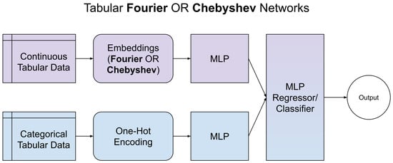
Figure 1.
Shared base architecture of TabFourierNet and TabChebyshevNet.
Building upon these specialized encoders, we propose two integrated architectures: PNPNet and AutoPNPNet. The PNPNet architecture involves an a priori separation of input features into periodic and non-periodic categories based on domain knowledge or statistical analysis. The periodic features are processed through the Fourier encoder, while the non-periodic features pass through the Chebyshev encoder. Outputs from both branches are then combined for the final prediction. This explicit separation allows the model to tailor its representation learning to the nature of each feature type. Recognizing that manual feature separation may not always be feasible or accurate, AutoPNPNet feeds all features into the Fourier and Chebyshev encoders. An additional MLP layer learns to automatically weigh and select the most relevant features from each encoder, performing implicit feature selection and combination. This approach eliminates prior feature categorization and allows the model to learn the optimal representation adaptively. From PNPNet and AutoPNPNet, we obtain TabPNPNet and TabAutoPNPNet, which process categorical data on a separate branch to continuous data. Figure 2 and Figure 3 present the architecture of PNPNet and AutoPNPNet, respectively, highlighting how periodic and non-periodic feature encodings are integrated.
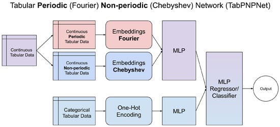
Figure 2.
Overview of the PNPNet architecture.
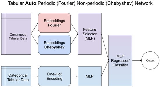
Figure 3.
Overview of the AutoPNPNet architecture.
3.1. FourierNet: Capturing Periodic Patterns
The Fourier-based neural encoder transforms input features into a frequency-domain representation, enabling the network to learn effectively from periodic components in the data. This highly configurable encoder allows for various options, such as input scaling, convolutional preprocessing, different activation functions, learnable frequencies, phase shifts, amplitudes, and Random Fourier Features (RFFs). Given an input feature vector , the encoder processes through several optional steps before applying the Fourier transformation. If input scaling is enabled, each input feature is scaled by a learnable parameter :
where ⊙ denotes element-wise multiplication. This scaling allows the model to adjust the influence of each feature. An optional one-dimensional convolutional layer can be applied to capture localized feature patterns:
where Conv1D represents a convolutional operation over the feature dimension with a specified kernel size.
The core of the Fourier encoder involves projecting the input features into a higher-dimensional space using sinusoidal functions. For each input feature , we associate m frequency components, forming a frequency matrix . Frequencies can be initialized using uniform, normal, or logarithmic initialization methods. If RFF is enabled, frequencies are sampled from a normal distribution, with variance inversely proportional to the bandwidth parameter :
Optionally, the encoder includes learnable amplitude and phase shift parameters for each feature and frequency component. The amplitude scaling is given by , and the phase shift is . The input features are projected using the frequencies, amplitudes, and phase shifts as follows:
The encoder supports several activation functions applied to projected inputs . For instance, with the sine and cosine activation (‘sin_cos’), the outputs are as follows:
These outputs are concatenated along the feature dimension. After activation, an optional learnable scaling parameter can be applied to encoded features:
The encoded features are then flattened to form the final encoded vector of dimension , where k depends on the activation function (e.g., for ‘sin_cos’, otherwise)
The overall architecture of FourierNet integrates the Fourier encoder with an MLP. The Fourier encoder transforms the input features into a higher-dimensional encoded representation , capturing periodic patterns through sinusoidal transformations with configurable frequencies, amplitudes, and phase shifts. This encoded representation is then processed by the MLP, which consists of L hidden layers. The operations of the MLP are defined as
where is an activation function (e.g., ReLU), and is appropriate for the task (e.g., linear activation for regression and softmax for classification).
Combining all components, the encoded feature for each input feature and frequency component j is given by
or according to the selected activation function. If the ‘sin_cos’ activation is used, the encoded features are
These features are then concatenated and flattened to form .
3.2. ChebyshevNet: Modeling Non-Periodic Patterns
To capture non-periodic, complex, non-linear relationships in tabular data, ChebyshevNet utilizes Chebyshev polynomials of the first kind. For each input feature , the Chebyshev polynomials are defined recursively:
A preliminary analysis of training trends revealed significant fluctuations in the loss values, which hindered the learning process, particularly for higher-degree polynomials that are more susceptible to numerical overflows. To address this issue, we explored feature clamping to enhance training stability. The input features are clamped to the interval :
The study on how this choice affects performance showed no significant change in accuracy for lower-degree polynomials, while it resulted in superior training stability for higher-degree polynomials.
The Chebyshev encoder generates an encoded feature tensor by computing the Chebyshev polynomials up to degree N for each input feature, resulting in a tensor of shape , where d is the number of input features:
A multi-headed encoding mechanism is introduced to enhance the encoder’s representative capacity. Let there be H heads in total. Each head processes the input features independently, with its own set of learnable parameters, including optional scaling factors , polynomial weights , and interaction kernels , where k is the kernel size.
For each head h, the input features may be scaled:
The Chebyshev polynomials are then computed for each scaled feature up to degree N. The weighted polynomials are obtained by applying the polynomial weights:
To model interactions among polynomial terms, the kernels are applied:
An activation function (e.g., SiLU) is applied to the result:
If residual connections are enabled, a residual from the input feature is added:
Each head produces an output tensor , representing the encoded features from that head. A cross-head attention mechanism is incorporated to capture dependencies between different heads. The output tensors from each head are flattened to form vectors:
Queries, keys, and values for each head are computed using linear projections:
where are learnable projection matrices, and is the attention dimension. The attention scores between heads are computed as
The attention weights are obtained via the softmax function:
The output of the cross-head attention for each head is calculated as
The outputs from all heads are concatenated to form the final encoded representation:
An optional normalization layer, such as Layer Normalization, may be applied to to stabilize training.
ChebyshevNet integrates the Chebyshev encoder with the multi-headed encoding and cross-head attention mechanisms. The overall architecture begins with input processing, where input features may be scaled and clamped to for numerical stability. The multi-headed encoding then computes the weighted Chebyshev polynomials and applies the kernels for each head, including activation functions and residual connections as configured. Following encoding, the cross-head attention mechanism processes the outputs of all heads, computing queries, keys, values, and attention weights to combine the value vectors. The attended outputs of all heads are concatenated, and optional normalization is applied to the combined representation. The final encoded representation is passed through an MLP:
Here, is an activation function (e.g., ReLU), and is the output function appropriate for the task.
3.3. PNPNet: Periodic-Non-Periodic Network
PNPNet requires an initial separation of the input features into periodic and non-periodic subsets, denoted as and , respectively, where . This separation can be based on domain knowledge or statistical analysis techniques, such as spectral density estimation or autocorrelation analysis.
PNPNet consists of two parallel branches that process the periodic and non-periodic features separately. The periodic features are transformed using the Fourier encoder to obtain , which is then processed by an MLP specific to the periodic branch:
Similarly, the non-periodic features are transformed using the Chebyshev encoder to obtain , processed by the non-periodic branch MLP:
The outputs from both branches are concatenated to form the fused representation:
This fused representation is then passed through a final MLP to produce the prediction:
3.4. AutoPNPNet: Automatic Feature Selection
AutoPNPNet addresses the challenge of manually separating features into periodic and non-periodic categories by simultaneously feeding all input features into the Fourier and Chebyshev encoders. This approach allows the model to learn which features are best represented by each encoder in a data-driven manner. The input features are processed as follows:
Here, and are the encoded representations produced by the Fourier and Chebyshev encoders, respectively, where and are the dimensions of the encoded feature spaces.
The encoded representations from both encoders are processed through their respective MLPs to capture complex interactions and feature transformations:
Here, and are the outputs of the Fourier and Chebyshev branches after the and layers, respectively.
An attention mechanism is employed to learn the optimal weighting between the two branches, enabling the model to determine the importance of periodic and non-periodic features automatically. The attention weights and are computed as
where and are learnable parameters, and the softmax function ensures that and .
The fused representation is then computed as a weighted sum of the outputs from the two branches:
This fusion allows the model to emphasize the features and patterns most relevant for the prediction task based on the learned attention weights.
The fused representation is then passed through a final MLP to produce the prediction :
Here, and are the weights and biases of the final MLP layer, is an activation function (e.g., ReLU), and is the output function appropriate for the task (e.g., linear activation for regression, softmax for classification).
In some configurations, AutoPNPNet may include a cross-attention mechanism to capture further interactions between the features encoded by the Fourier and Chebyshev encoders. The cross-attention allows the model to attend to the combined representations, enhancing the ability to model complex dependencies.
Given the projected representations and obtained from the encoded features,
where and are projection matrices that correspond to a shared embedding space of dimension .
The combined representations are concatenated and passed through a multi-head attention layer:
where captures the attended features, and the multi-head attention mechanism allows the model to focus on different aspects of the combined representations.
The attended features are then processed through additional layers, including a linear transformation and an activation function, and normalization as follows:
An aggregation operation, such as averaging, is applied across the sequence dimension to obtain a fixed-size representation:
This representation is then used in place of or in addition to for the final prediction layer.
3.5. Training Objective
The training objective depends on the nature of the task.
For regression, we minimize the Mean Squared Error (MSE) loss:
where n is the number of samples, is the true target, and is the predicted value.
For classification, we minimize the Cross-Entropy loss:
where K is the number of classes, is the binary indicator (1 if sample i belongs to class k, 0 otherwise), and is the predicted probability that sample i belongs to class k.
3.6. Implementation Details
We use the Rectified Linear Unit (ReLU) activation function defined as
Input features are normalized to have a zero mean and unit variance. We employ batch normalization after each fully connected layer to improve training stability and convergence. We employ the Adam optimizer [50] with default parameters for training. The update rule for the parameters is
where is the learning rate, and are the bias-corrected first and second moment estimates, and is a small constant to prevent division by zero. To avoid overfitting, we apply dropout regularization and L2 weight decay. Dropout randomly zeros a fraction of the neurons during training, reducing neuron co-adaptation. L2 regularization adds a penalty proportional to the square of the weights to the loss function.
3.7. Computational Complexity Analysis
The encoders introduce additional computational overhead compared to standard MLPs. The computational complexity of the Fourier encoder is , where d is the number of input features and m is the number of frequency components. The computational complexity of the Chebyshev encoder is , where N is the maximum degree of the Chebyshev polynomials.
3.8. Periodicity Detection
Detecting periodic patterns in data is crucial for effectively modeling and forecasting time series and other datasets with cyclical behaviors. Accurate identification of periodicity allows models to incorporate appropriate transformations and encodings, such as Fourier transforms, to capture these patterns. This section discusses a method for detecting periodicity in time series data using the autocorrelation function (ACF) and peak detection algorithms. The ACF measures the correlation of a signal with a delayed copy of itself as a function of the delay (lag). For a discrete time series , the autocorrelation at lag k is defined as
where is the mean of the series, and k is the lag. The ACF provides insight into the repeating patterns within the data by highlighting the lags in which the series is correlated with itself. Periodic time series exhibit significant autocorrelations at lags corresponding to their period and multiples. By analyzing the peaks in the ACF, we can infer the presence of periodicity and estimate the period length. To detect periodicity using the ACF, we first calculate the ACF of the time series up to a specified maximum lag . The should cover at least one expected period. Next, we identify significant peaks in the ACF using a peak detection algorithm. Peaks represent lags where the autocorrelation is locally maximal and exceeds certain thresholds in height and prominence. Specifically, peaks must have a height above a minimum value to be considered significant, and they must stand out relative to neighbouring values, measured by the prominence parameter . Additionally, peaks must be separated by at least a minimum number of lags to avoid closely spaced false positives. After identifying the peaks, we analyze the distances between consecutive peaks, denoted as , where is the lag of the k-th peak. If the series is periodic, these distances should be approximately constant, corresponding to the period of the series. We assess periodicity by determining whether the standard deviation of the peak distances is below a certain threshold . A low standard deviation indicates that the peaks occur at regular intervals, supporting the presence of periodicity. Let be the autocorrelation values excluding lag zero. The peak detection algorithm identifies the set of peak lags satisfying the following conditions:
The standard deviation of the peak distances is computed as follows:
where N is the number of detected peaks and is the mean of the peak distances. Periodicity is detected if .
The following pseudocode Algorithm 1 summarizes the steps of the periodicity detection algorithm using the ACF and peak detection:
| Algorithm 1 Periodicity Detection using ACF Peaks |
| Require: Time series data Require: Parameters: maximum lag , minimum peak height , minimum peak prominence , minimum distance between peaks , standard deviation threshold Ensure: Boolean value indicating whether periodicity is detected
|
4. Datasets
We utilize a benchmark of 53 tabular datasets encompassing regression and classification tasks [2]. These datasets cover various domains and vary in the number of samples, feature types, and complexity as shown in Table 1, Table 2, Table 3 and Table 4. We categorize the datasets for analysis based on task type and feature composition. The task types include regression tasks, which involve predicting continuous target variables, and classification tasks, which involve predicting categorical target variables. The feature compositions include datasets containing exclusively numerical features and a mix of numerical and categorical features. This categorization allows us to assess the performance of our models under different data conditions.

Table 1.
Statistics of benchmark datasets for numerical classification.
Table 2.
Statistics of benchmark datasets for numerical regression.
Table 3.
Statistics of benchmark datasets for categorical classification.
Table 4.
Statistics of benchmark datasets for categorical regresssion.
We follow the data preprocessing protocols outlined in the benchmark study. Missing values are imputed using the mean for numerical features and the mode for categorical features. Categorical variables are processed using embedding layers within the models, consistent with FT-Transformer’s methodology. The numerical features are standardized to have zero mean and unit variance.
5. Experiments
Our experiments are designed to address four key research questions:
- RQ1: Do FourierNet and ChebyshevNet (and respective Tab versions) individually outperform FT-Transformer on the benchmark?
- RQ2: Does integrating periodic and non-periodic encoders in PNPNet and AutoPNPNet (and respective Tab versions) lead to further performance gains compared to FT-Transformer?
- RQ3: How does AutoPNPNet’s automatic feature selection mechanism compare to the manual feature separation employed in PNPNet?
- RQ4: What is the trade-off between the computational overhead introduced by the specialized encoders and the performance improvements achieved?
As discussed in Section 4, we assess the performance of our proposed models on a comprehensive benchmark of tabular datasets spanning both regression and classification tasks, including continuous numerical and categorical features. We test our FourierNet, ChebyshevNet, PNPNet, and AutoPNPNet models for datasets including only continuous numerical features. We test our TabFourierNet, TabChebyshevNet, TabPNPNet, and TabAutoPNPNet models for datasets including continuous numerical and categorical features. We compare our models against FT-Transformer, the SoA baseline for the DL method operating on tabular data (Our reference implementation of FT-Transformer is presented in Gorishniy et al. [8], and offers a straightforward open-source implementation, available at https://github.com/yandex-research/rtdl-revisiting-models) (accessed on 10 March 2025). We deliberately omit other DL baselines, since FT-Transformer beats them on the examined benchmark, and other tree-based models, as they are far superior to deep models, as extensively discussed in Grinsztajn et al. [2].
To ensure robust evaluation, we perform five-fold cross-validation on each dataset. All models, including FT-Transformer and our proposed architectures, are configured with comparable hyperparameters to ensure a fair comparison. Each model uses four hidden layers for the MLP components, with 256 neurons per hidden layer. The ReLU activation function is employed for hidden layers, linear activation for regression tasks, and softmax for classification tasks. The models are optimized using the Adam optimizer with a learning rate of 0.001. The batch size is set to 1024 samples, and training proceeds for up to 100 epochs with early stopping based on validation loss with patience equal to 10. Regularization techniques include a dropout rate of 0.1 and L2 weight decay with a coefficient of 0.0001. For our specialized encoders, the Fourier encoder uses 20 frequency components, with frequencies selected based on the range of the input features. The Chebyshev encoder has a maximum polynomial degree of 10. The attention mechanism in AutoPNPNet is implemented using a gating mechanism with learnable parameters.
We employ standard evaluation metrics suitable for regression and classification tasks. For regression tasks, we use Mean Squared Error (MSE), Root Mean Squared Error (RMSE), Mean Absolute Error (MAE), and the Coefficient of Determination ( Score). We use Accuracy, Precision, Recall, and F1-Score for classification tasks. The tables in the following sections report the improved metrics for each task and dataset, the model that reported the improvement, and a percentage of improvement over the baseline FT-Transformer. Such an improvement percentage is computed by analyzing each metric’s mean and standard deviation across the five folds.
6. Results
6.1. Regression Tasks
Table 5 and Table 6 present our model’s performance improvements for the categorical and numerical regression tasks, respectively. Our models outperform FT-Transformer in at least one metric for 9/13 datasets containing categorical and continuous numerical features, and 12/20 datasets with continuous numerical features only.
Table 5.
Performance improvement of models across datasets for categorical regression.
Table 6.
Performance improvement of models across datasets for numerical regression.
6.2. Classification Tasks
Table 7 and Table 8 present our model’s performance improvements for the categorical and numerical classification tasks, respectively. In classification tasks involving categorical and continuous numerical features, our models surpass FT-Transformer on 4/7 datasets. In classification tasks involving continuous numerical features only, our models beat the baseline on 9/13 datasets.
Table 7.
Performance improvement of models across datasets for categorical classification.
Table 8.
Performance improvement of models across datasets for numerical classification.
6.3. Discussion
The results demonstrate that our proposed models report performance gains over the baseline for 34 out of 52 datasets across multiple regression and classification tasks, regardless of the feature composition. FourierNet and ChebyshevNet individually show improvements over FT-Transformer in numerous scenarios, validating the effectiveness of their specialized encoders. Performance gains are observed in datasets with numerical features only and with both numerical and categorical features, highlighting the versatility of our models. Preliminary single-dataset ablation studies suggested the effectiveness of the PNPNet architecture over FourierNet and ChebyshevNet, as well as the superior performance of AutoPNPNet. However, the here-reported extensive benchmarking demonstrates that the actual best architecture depends on the specific scenario. In most cases, the combined architectures, PNPNet and AutoPNPNet, achieve the highest performance, suggesting that integrating periodic and non-periodic encoders enhances the models’ ability to capture complex patterns inherent in tabular data. AutoPNPNet results in marginal but consistent performance improvements over PNPNet, indicating the effectiveness of automatic feature selection in capturing subtle patterns that manual separation might miss. We reckon the computational costs of our models in terms of training time and parameter count. Although our models introduce additional computational overhead due to the specialized encoders, the training times remain manageable. Performance gains justify the extra computational cost, particularly in applications where predictive accuracy is critical. The specialized encoders increase the number of parameters and slightly prolong training time per epoch, but these increases are fair to the improvements in model performance.
Addressing the first research question, FourierNet and ChebyshevNet individually outperform FT-Transformer on multiple benchmark datasets. This demonstrates the effectiveness of specialized encoders in capturing specific data characteristics. Regarding the second question, PNPNet and AutoPNPNet achieve further improvements over the FT-Transformer and the individual models. Integrating both encoders enables the models to capture a broader range of patterns, enhancing performance. For the third question, AutoPNPNet consistently outperforms PNPNet by a small margin. The automatic feature selection mechanism allows the model to adaptively learn the importance of the features, potentially capturing subtle patterns that manual separation might overlook. Concerning the fourth question, while the specialized encoders increase computational overhead, our models balance computational efficiency and predictive accuracy.
7. Explainability
Understanding the decisions made by ML models is crucial, particularly in domains where explainability is as vital as predictive accuracy. Our proposed models—FourierNet, ChebyshevNet, PNPNet, and AutoPNPNet—aim to enhance predictive performance and improve explainability by leveraging specialized neural encoders that capture specific data patterns. This section delves into how these models provide opportunities for feature importance analysis and facilitate a deeper understanding of the underlying data structures. By leveraging periodicity through Fourier and Chebyshev encodings, we introduce a structured and mathematically grounded transformation that enhances model expressiveness and explainability. Fourier encodings capture cyclical patterns in data, making them particularly effective for time series and periodic features. At the same time, Chebyshev polynomials provide a flexible approximation that can reveal complex yet structured relationships between input variables. These encodings create feature transformations that connect directly to the original feature space, allowing practitioners to interpret learned representations in frequency components or polynomial expansions. The specialized encoders in our models transform input features into representations that allow us to analyze the influence of individual features and their transformations on the model’s predictions. The Fourier encoder captures periodic patterns by transforming features into frequency components, while the Chebyshev encoder captures non-linear relationships through polynomial expansions. This explicit representation of patterns allows us to interpret which features and patterns are most significant in the model decision-making process.
In FourierNet, each input feature is associated with a set of frequency components due to Fourier encoding. By examining the learned weights associated with these components in the layers of the neural network following the encoder, we can assess the importance of different frequencies for each feature. For instance, if specific frequencies have higher weights, the corresponding periodic patterns in the feature significantly influence the model’s output. This provides an avenue to identify and interpret the periodic behavior of features that contribute most to the predictions. Mathematically, consider the Fourier-encoded feature vector . The network learns weights in each layer l that are applied to . By analyzing the magnitude of these weights, specifically those connected to the frequency components, we can quantify the impact of each frequency. Features whose frequency components are associated with larger weights are deemed more important. This analysis can be visualized by plotting the weight magnitudes against the frequencies, highlighting dominant periodicities.
ChebyshevNet employs the Chebyshev encoder to expand the features into a series of Chebyshev polynomials. Each feature is represented by its polynomial terms up to a certain degree, capturing various levels of non-linearity. Analyzing the weights associated with these polynomial terms in the subsequent neural network layers allows us to determine the significance of different degrees of non-linearity for each feature. Features whose higher-degree polynomial terms have substantial weights are influential due to their complex non-linear relationships with the target variable. For each input feature , the Chebyshev encoder produces terms for . The network learns weights connecting these terms to the output. By examining these weights, we can identify the degrees of polynomial expansion that are most impactful. A high weight on suggests that the n-th degree non-linear transformation of plays a significant role in the model’s predictions.
PNPNet combines the Fourier and Chebyshev encoders, processing periodic and non-periodic features separately. This explicit separation enhances explainability by enabling us to analyze the contributions of each type of feature independently. By examining the weights and activations in each branch, we can identify which features, whether periodic or non-periodic, are most important for the model’s predictions. In the periodic branch, the importance of frequency components for periodic features can be assessed as in FourierNet. The significance of polynomial degrees for non-periodic features can be analyzed in the non-periodic branch as in ChebyshevNet. Additionally, the outputs of both branches before fusion provide insights into the relative importance of periodic versus non-periodic features. If activations from one branch dominate the fused representation, it suggests that the corresponding feature type has a greater influence on the prediction.
AutoPNPNet extends explainability by automatically incorporating an attention mechanism that learns to weigh the importance of features from both the Fourier and Chebyshev encoders. The attention weights assigned to each encoder’s output reflect the model’s assessment of the significance of periodic and non-periodic patterns in making predictions. By analyzing these attention weights, we can infer whether the model relies more on periodic features, non-periodic features, or a combination of both for a given task.
The attention mechanism computes weights and for the Fourier and Chebyshev branches, respectively:
where and . These weights directly indicate the model’s emphasis on each type of encoded feature. A higher suggests that periodic patterns captured by the Fourier encoder are more critical, while a higher indicates the importance of non-linear relationships captured by the Chebyshev encoder.
To further enhance feature importance analysis, we can employ gradient-based attribution methods. By computing the gradients of the model’s output with respect to each input feature, we can quantify the prediction’s sensitivity to changes in each feature. In the context of our models, this gradient analysis can be applied to the encoded features produced by the Fourier and Chebyshev encoders. This allows us to identify important features and understand how specific transformations of these features (e.g., certain frequency components or polynomial terms) affect the output. For each input feature , the gradient indicates how small changes in the feature affect the output. In our models, this gradient can be decomposed to assess the contribution of each encoded component:
where represents the k-th encoded component (frequency component or polynomial term). This decomposition allows us to attribute the importance of the output to specific transformations of the input features.
Additionally, visualization of the learned feature representations can aid in explainability. For example, in FourierNet, plotting the magnitude of the learned weights associated with different frequency components can reveal dominant periodic patterns in the data. In ChebyshevNet, examining the weights of polynomial terms can highlight the degree of non-linearity the model deems important for each feature. Such visualizations can provide intuitive insights into the model’s behaviour and the underlying data structures. In practical applications, understanding which features and patterns influence the model’s predictions can inform domain experts and support decision-making processes. For instance, identifying that certain periodic components of a feature are highly influential in a time series forecasting task can lead to a better understanding of seasonal effects. In regression tasks involving complex systems, recognizing that higher-degree polynomial terms of certain features are significant can indicate the presence of non-linear dynamics. Our models’ architecture facilitates feature importance analysis not only at the level of individual features, but also at the level of specific patterns captured by the encoders. This multi-level explainability is a key advantage over traditional neural networks, where the transformations applied to input features are often less transparent. By providing explicit representations of periodic and non-linear patterns, our models make it possible to dissect and understand the contributions of different aspects of the data to the final prediction.
8. Limitations and Future Work
Our study acknowledges certain limitations. The performance of the specialized encoders may depend on hyperparameter choices such as the number of frequency components and the degree of Chebyshev polynomials, indicating hyperparameter sensitivity. For extremely large datasets, the increase in the number of parameters may lead to longer training times and higher memory requirements, posing scalability challenges. While our models handle categorical features using embeddings, the specialized encoders are primarily designed for numerical data, and extending their capabilities to integrate categorical features better remains an area for future work.
Potential directions for future research include developing methods to learn the optimal number of frequency components and polynomial degrees during training, thereby adapting encoder parameters. Extending specialized encoders to process categorical features, possibly through categorical-specific transformations more effectively, would enhance categorical feature integration. Exploring techniques to reduce computational overhead, such as pruning or quantization, without significantly impacting performance could lead to model compression. Combining our approach with other advanced models, such as attention mechanisms or graph neural networks, to further improve performance on tabular data represents a potential for hybrid architectures.
9. Conclusions
This paper introduced novel neural network architectures to enhance tabular data modelling by capturing inherent periodic and non-linear patterns. FourierNet employs a Fourier-based encoder to capture periodic relationships within the data. The model effectively identifies and leverages periodic patterns common in time series and other cyclical data by transforming features into frequency components. ChebyshevNet, on the other hand, utilizes a Chebyshev polynomial-based encoder to model complex non-linear relationships. This approach allows the model to approximate intricate functions and interactions that standard neural networks might miss. Based on these foundations, PNPNet combines Fourier and Chebyshev encoders to handle periodic and non-periodic features simultaneously. PNPNet enhances the model’s capacity to capture a broader range of patterns by explicitly separating and processing these feature types. AutoPNPNet advances this concept further by introducing an attention mechanism that automatically learns the importance of periodic and non-periodic features, eliminating the need for manual feature separation and allowing the model to focus on the most relevant patterns in the data adaptively. Our experimental evaluation on a comprehensive benchmark of 53 tabular datasets demonstrated that our models outperform the SoA DL baseline across regression and classification tasks in 34 cases. The performance gains were observed in datasets containing only numerical features and those with a mix of numerical and categorical features. The results validate the effectiveness of our specialized encoders in capturing essential data characteristics and improving predictive accuracy. Moreover, we explored the explainability aspects of our models, highlighting how the specialized encoders facilitate feature importance analysis. We can interpret the influence of specific patterns and features on the model’s predictions by examining the learned weights associated with frequency components in FourierNet and polynomial degrees in ChebyshevNet. AutoPNPNet’s attention mechanism provides additional insights by indicating the relative importance of periodic versus non-periodic features. These explainability features are crucial for applications where understanding the rationale behind model decisions is essential.
Author Contributions
Conceptualization, M.R., E.A., A.A. and A.G.; methodology, M.R.; software, M.R.; validation, M.R., E.A. and A.A.; formal analysis, M.R.; investigation, M.R.; resources, E.A.; data curation, M.R.; writing—original draft preparation, M.R.; writing—review and editing, M.R., E.A., A.A. and A.G.; visualization, M.R.; supervision, A.A. and A.G.; project administration, M.R.; funding acquisition, A.A. All authors have read and agreed to the published version of the manuscript.
Funding
This paper was funded by Veneto Agricoltura within the scope of the project “Guaranteeing the continuity of the agri-foodchain: the digitization of wholesale markets”.
Data Availability Statement
The original data presented in the study are openly available at https://github.com/matteo-rizzo/periodic-tabular-dl (accessed on 10 March 2025).
Conflicts of Interest
The authors declare no conflicts of interest.
References
- Shwartz-Ziv, R.; Armon, A. Tabular data: Deep learning is not all you need. arXiv 2021, arXiv:2106.03253. [Google Scholar] [CrossRef]
- Grinsztajn, L.; Oyallon, E.; Varoquaux, G. Why do tree-based models still outperform deep learning on typical tabular data? Adv. Neural Inf. Process. Syst. 2022, 35, 507–520. [Google Scholar]
- Zhu, Y.; Brettin, T.; Xia, F.; Partin, A.; Shukla, M.; Yoo, H.; Evrard, Y.A.; Doroshow, J.H.; Stevens, R.L. Converting tabular data into images for deep learning with convolutional neural networks. Sci. Rep. 2021, 11, 11325. [Google Scholar] [CrossRef]
- Katzir, L.; Elidan, G.; El-Yaniv, R. Net-dnf: Effective deep modeling of tabular data. In Proceedings of the International Conference on Learning Representations, Addis Ababa, Ethiopia, 30 April 2020. [Google Scholar]
- Arık, S.Ö.; Pfister, T. TabNet: Attentive interpretable tabular learning. In Proceedings of the AAAI Conference on Artificial Intelligence, Online, 2–9 February 2021; Volume 35, pp. 6679–6687. [Google Scholar]
- Popov, S.; Morozov, S.; Babenko, A. Neural oblivious decision ensembles for deep learning on tabular data. In Proceedings of the Advances in Neural Information Processing Systems, Vancouver, BC, Canada, 8–14 December 2019; Volume 32. [Google Scholar]
- Ke, G.; Zheng, H.; Chen, H.; Liu, T.Y. DeepGBM: A deep learning framework distilled by GBDT for online prediction tasks. In Proceedings of the 25th ACM SIGKDD International Conference on Knowledge Discovery & Data Mining, Anchorage, AK, USA, 4–8 August 2019; pp. 384–394. [Google Scholar]
- Gorishniy, Y.; Rubachev, I.; Khrulkov, V.; Babenko, A. Revisiting deep learning models for tabular data. In Proceedings of the Advances in Neural Information Processing Systems, Online, 6–14 December 2021; Volume 34, pp. 18932–18943. [Google Scholar]
- Gorishniy, Y.; Rubachev, I.; Babenko, A. On embeddings for numerical features in tabular deep learning. Adv. Neural Inf. Process. Syst. 2022, 35, 24991–25004. [Google Scholar]
- Ren, W.; Zhao, T.; Huang, Y.; Honavar, V. Deep Learning within Tabular Data: Foundations, Challenges, Advances and Future Directions. arXiv 2025, arXiv:2501.03540. [Google Scholar]
- Domingo-Ferrer, J.; Vi, T.; Vi, D.; Vil, D. Tabular Data; Springer: Boston, MA, USA, 2018. [Google Scholar] [CrossRef]
- Rizzo, M.; Veneri, A.; Albarelli, A.; Lucchese, C.; Nobile, M.; Conati, C. A Theoretical Framework for AI Models Explainability with Application in Biomedicine. In Proceedings of the 2023 IEEE Conference on Computational Intelligence in Bioinformatics and Computational Biology (CIBCB), Eindhoven, The Netherlands, 29–31 August 2023; pp. 1–9. [Google Scholar] [CrossRef]
- Rizzo, M.; Marcuzzo, M.; Zangari, A.; Schiavinato, M.; Albarelli, A.; Gasparetto, A. Stop Overkilling Simple Tasks with Black-Box Models, Use More Transparent Models Instead. In Proceedings of the Pattern Recognition and Artificial Intelligence, Jeju Island, Republic of Korea, 3–6 July 2024; Wallraven, C., Liu, C.L., Ross, A., Eds.; Springer: Singapore, 2025; pp. 279–293. [Google Scholar]
- Goodfellow, I.; Bengio, Y.; Courville, A. Deep Learning; MIT Press: Cambridge, MA, USA, 2016. [Google Scholar]
- Friedman, J.H. Greedy function approximation: A gradient boosting machine. Ann. Stat. 2001, 29, 1189–1232. [Google Scholar] [CrossRef]
- Breiman, L. Random forests. Mach. Learn. 2001, 45, 5–32. [Google Scholar] [CrossRef]
- Huang, X.; Khetan, A.; Cvitkovic, M.; Karnin, Z. TabTransformer: Tabular data modeling using contextual embeddings. arXiv 2020, arXiv:2012.06678. [Google Scholar]
- Banerjee, R.; Bhattacharya, S.K. Data: Periodicity and Ways to Unlock Its Full Potential. In Rhythmic Advantages in Big Data and Machine Learning; Springer: Singapore, 2022; pp. 1–22. [Google Scholar]
- Yang, Y.; Xiong, Z.; Liu, T.; Wang, T.; Wang, C. Fourier Learning with Cyclical Data. In Proceedings of the International Conference on Machine Learning, Baltimore, MD, USA, 17–23 July 2022; pp. 25280–25301. [Google Scholar]
- Rahimi, A.; Recht, B. Random features for large-scale kernel machines. In Proceedings of the Advances in Neural Information Processing Systems, Vancouver, BC, Canada, 3–6 December 2007; Volume 20. [Google Scholar]
- Vaswani, A.; Shazeer, N.; Parmar, N.; Uszkoreit, J.; Jones, L.; Gomez, A.N.; Kaiser, Ł.; Polosukhin, I. Attention is all you need. In Proceedings of the Advances in Neural Information Processing Systems, Long Beach, CA, USA, 4–9 December 2017; Volume 30. [Google Scholar]
- Sitzmann, V.; Martel, J.; Bergman, A.; Lindell, D.; Wetzstein, G. Implicit neural representations with periodic activation functions. In Proceedings of the Advances in Neural Information Processing Systems, Virtual, 6–12 December 2020; Volume 33, pp. 7462–7473. [Google Scholar]
- Rivlin, T.J. The Chebyshev Polynomials; Wiley-Interscience: Hoboken, NJ, USA, 1974. [Google Scholar]
- Sidharth, S.S.; Keerthana, A.R.; Gokul, R.; Anas, K.P. Chebyshev polynomial-based kolmogorov-arnold networks: An efficient architecture for nonlinear function approximation. arXiv 2024, arXiv:2405.07200. [Google Scholar]
- Defferrard, M.; Bresson, X.; Vandergheynst, P. Convolutional neural networks on graphs with fast localized spectral filtering. In Proceedings of the Advances in Neural Information Processing Systems, Barcelona, Spain, 5–10 December 2016; Volume 29. [Google Scholar]
- Trefethen, L.N. Approximation Theory and Approximation Practice; SIAM: New Delhi, India, 2013. [Google Scholar]
- Chen, Y.; Zheng, L.; Ali, M.; Zhang, J. Learning deep representations for the multi-branch neural networks. IEEE Trans. Neural Netw. Learn. Syst. 2019, 30, 2396–2406. [Google Scholar]
- Cherepanova, V.; Levin, R.; Somepalli, G.; Geiping, J.; Bruss, C.B.; Wilson, A.G.; Goldstein, T.; Goldblum, M. A performance-driven benchmark for feature selection in tabular deep learning. Adv. Neural Inf. Process. Syst. 2023, 36, 41956–41979. [Google Scholar]
- Bahdanau, D.; Cho, K.; Bengio, Y. Neural machine translation by jointly learning to align and translate. In Proceedings of the International Conference on Learning Representations, San Diego, CA, USA, 7–9 May 2015. [Google Scholar]
- Pham, H.; Tan, Y.; Singh, T.; Pavlopoulos, V.; Patnayakuni, R. A multi-head attention-like feature selection approach for tabular data. Knowl.-Based Syst. 2024, 301, 112250. [Google Scholar] [CrossRef]
- Tibshirani, R. Regression shrinkage and selection via the lasso. J. R. Stat. Soc. Ser. B (Methodol.) 1996, 58, 267–288. [Google Scholar] [CrossRef]
- Li, Z.; Liu, B.; Tang, J. Robust structured subspace learning for data representation. IEEE Trans. Pattern Anal. Mach. Intell. 2015, 37, 2085–2098. [Google Scholar] [CrossRef] [PubMed]
- Amballa, A.; Akkinapalli, G.; Madine, M.; Yarrabolu, N.P.P.; Grabowicz, P.A. Automated model selection for tabular data. arXiv 2024, arXiv:2401.00961. [Google Scholar]
- MacKay, D.J.C. Bayesian methods for backpropagation networks. In Models of Neural Networks III; Springer: New York, NY, USA, 1994; pp. 211–254. [Google Scholar]
- Gunning, D.; Stefik, M.; Choi, J.; Miller, T.; Stumpf, S.; Yang, G.Z. XAI—Explainable artificial intelligence. Sci. Robot. 2019, 4, eaay7120. [Google Scholar] [CrossRef]
- Adadi, A.; Berrada, M. Peeking Inside the Black-Box: A Survey on Explainable Artificial Intelligence (XAI). IEEE Access 2018, 6, 52138–52160. [Google Scholar] [CrossRef]
- Sahakyan, M.; Aung, Z.; Rahwan, T. Explainable Artificial Intelligence for Tabular Data: A Survey. IEEE Access 2021, 9, 135392–135422. [Google Scholar] [CrossRef]
- O’Brien Quinn, H.; Sedky, M.; Francis, J.; Streeton, M. Literature review of explainable tabular data analysis. Electronics 2024, 13, 3806. [Google Scholar] [CrossRef]
- Wa, S.; Lu, X.; Wang, M. Stable and Interpretable Deep Learning for Tabular Data: Introducing InterpreTabNet with the Novel InterpreStability Metric. arXiv 2023, arXiv:2310.02870. [Google Scholar]
- Ullah, I.; Rios, A.; Gala, V.; Mckeever, S. Explaining deep learning models for tabular data using layer-wise relevance propagation. Appl. Sci. 2021, 12, 136. [Google Scholar] [CrossRef]
- Wani, N.A.; Kumar, R.; Bedi, J.; Rida, I. Explainable AI-driven IoMT fusion: Unravelling techniques, opportunities, and challenges with Explainable AI in healthcare. Inf. Fusion 2024, 110, 102472. [Google Scholar] [CrossRef]
- Weber, P.; Carl, K.V.; Hinz, O. Applications of explainable artificial intelligence in finance—A systematic review of finance, information systems, and computer science literature. Manag. Rev. Q. 2024, 74, 867–907. [Google Scholar] [CrossRef]
- Černevičienė, J.; Kabašinskas, A. Explainable artificial intelligence (XAI) in finance: A systematic literature review. Artif. Intell. Rev. 2024, 57, 216. [Google Scholar] [CrossRef]
- Kostopoulos, G.; Davrazos, G.; Kotsiantis, S. Explainable Artificial Intelligence-Based Decision Support Systems: A Recent Review. Electronics 2024, 13, 2842. [Google Scholar] [CrossRef]
- Wang, A.X.; Chukova, S.S.; Simpson, C.R.; Nguyen, B.P. Challenges and opportunities of generative models on tabular data. Appl. Soft Comput. 2024, 166, 112223. [Google Scholar] [CrossRef]
- Hancock, J.T.; Khoshgoftaar, T.M. Survey on categorical data for neural networks. J. Big Data 2020, 7, 28. [Google Scholar] [CrossRef]
- Fitkov-Norris, E.; Vahid, S.; Hand, C. Evaluating the impact of categorical data encoding and scaling on neural network classification performance: The case of repeat consumption of identical cultural goods. In Proceedings of the Engineering Applications of Neural Networks: 13th International Conference, EANN 2012, London, UK, 20–23 September 2012; Proceedings 13. Springer: Berlin/Heidelberg, Germany, 2012; pp. 343–352. [Google Scholar]
- Wu, Y.; Luo, H.; Lee, R.S. Deep feature embedding for tabular data. arXiv 2024, arXiv:2408.17162. [Google Scholar]
- Christoph, M. Interpretable Machine Learning: A Guide for Making Black Box Models Explainable; Leanpub: Victoria, BC, Canada, 2020. [Google Scholar]
- Kingma, D.P.; Ba, J. Adam: A method for stochastic optimization. arXiv 2014, arXiv:1412.6980. [Google Scholar]
Disclaimer/Publisher’s Note: The statements, opinions and data contained in all publications are solely those of the individual author(s) and contributor(s) and not of MDPI and/or the editor(s). MDPI and/or the editor(s) disclaim responsibility for any injury to people or property resulting from any ideas, methods, instructions or products referred to in the content. |
© 2025 by the authors. Licensee MDPI, Basel, Switzerland. This article is an open access article distributed under the terms and conditions of the Creative Commons Attribution (CC BY) license (https://creativecommons.org/licenses/by/4.0/).