Abstract
Industrial robots play a crucial role in modern manufacturing, but ensuring safe human–robot collaboration remains a challenge. Traditional collision avoidance methods, such as physical barriers and emergency stops, are limited in efficiency and flexibility. This study proposes the Asymmetry Elliptical Likelihood Potential Field (AELPF) algorithm, a novel real-time collision avoidance system inspired by autonomous driving technologies. The AELPF method leverages LiDAR sensors to dynamically compute an asymmetric elliptical repulsive field, enabling precise obstacle detection and avoidance in 3D environments. Unlike conventional potential field approaches, the AELPF accounts for both vertical and horizontal deviations, allowing it to adapt to complex industrial settings. To quantify the performance of AELPF, we compare it to two commonly used algorithms: the Vector Field Histogram (VFH) and the Follow the Gap Method (FGM). In terms of processing time, the VFH algorithm requires 50 ms per cycle, while the FGM algorithm operates at 22 ms. In contrast, the the AELPF, when using only a single channel, processes at 12 ms, which is significantly faster than both the VFH and FGM. These results indicate that the AELPF not only provides faster decision-making but also ensures smoother, more responsive navigation in dynamic environments. Both simulation and physical experiments confirm that the AELPF significantly improves obstacle avoidance, particularly in the z-axis direction, reducing the risk of collisions while maintaining operational efficiency.
1. Introduction
Industrial robots have become indispensable in modern manufacturing, especially in high-precision and high-speed processes like injection molding [1]. The integration of robots into production lines has led to increased productivity, reduced labor costs, and minimized human exposure to hazardous tasks. According to recent studies, the use of industrial robots is linked to a significant reduction in workplace injuries. For instance, a study by Acemoglu and Restrepo [2] highlights that robot adoption in the U.S. has led to a 1.2 case per 100 worker reduction in injury rates. However, despite these advancements, concerns regarding the safety of human workers persist, particularly in environments where human–robot collaboration is frequent.
Various studies have been conducted to prevent collisions between robots and workers [3]. Traditionally, methods such as installing safety fences to physically limit the robot’s workspace or using emergency stop buttons to halt robot operations in case of a collision have been employed [4]. However, these approaches fundamentally restrict collaboration between robots and workers and negatively impact operational efficiency [5,6].
Recently, collision avoidance technologies utilizing vision systems and ultrasonic sensors have gained attention, enabling real-time maintenance of safety distances between workers and robots [7,8]. Nonetheless, these systems also face challenges, including insufficient real-time responsiveness and sensitivity to changes in the working environment.
Figure 1 [9] shows safety in industrial robot collaborative environments. While these existing safety technologies offer several advantages, they still have limitations when it comes to practical use in industrial settings. Specifically, as industrial robots work more closely with human workers in dynamic environments, the need for more sophisticated real-time avoidance systems becomes paramount. To address this challenge, several path planning and obstacle avoidance methods have been explored for industrial robotics, but each has its limitations:
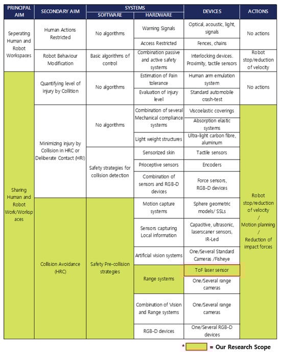
Figure 1.
Safety in industrial robot collaborative environments. The areas indicated in the figure represent the scope of our research [9].
RRT (Rapidly-exploring Random Tree) and RRT* (RRT Star) are pathfinding methods based on random sampling that excel at finding optimized paths in complex environments [10]. However, they generate numerous nodes during exploration, making real-time recalculation challenging and unsuitable for industrial applications where real-time performance is critical.
The Dynamic Window Approach (DWA) considers robot dynamics to sample candidate paths within feasible velocity and rotational speed ranges, making it effective for local obstacle avoidance [11]. However, in environments with numerous or dynamic obstacles, the increased number of sampled paths can lead to significant computational burden, potentially reducing real-time responsiveness.
Deep Reinforcement Learning-based obstacle avoidance is a modern AI-driven method allowing robots to autonomously learn in diverse environments [12,13]. While it offers adaptability, this approach requires retraining in new environments, demands large amounts of data and time during training, and struggles to guarantee stable performance.
Given these limitations, there is a clear need for more robust and efficient real-time obstacle avoidance systems that can meet the demands of dynamic industrial environments while ensuring worker safety. To address this, we drew inspiration from advancements in autonomous driving systems, which have proven highly effective in real-time obstacle detection and avoidance in complex, dynamic environments.
In particular, we considered the Obstacle-Dependent Gaussian Potential Field (ODGPF) algorithm, as it demonstrates some capability in navigating dynamic environments [14]. However, the ODGPF method is limited by its 2D application scope, making it less suitable for use with industrial articulated robots that operate in 3D environments. Additionally, the ODGPF may generate inefficient avoidance paths in densely populated obstacle regions, which could reduce effectiveness in industrial settings.
Therefore, in this research, we propose a novel collision avoidance system, the Asymmetry Elliptical Likelihood Potential Field, AELPF. This system applies the principles of autonomous driving avoidance technology to industrial robots, providing a safer and more flexible solution for environments where robots and humans work simultaneously. By collecting real-time 3D environmental information through LiDAR sensors and calculating collision possibilities with obstacles using the asymmetry elliptical repulsive field, the robot can quickly and accurately adjust its path. This represents a more advanced approach compared to traditional reliance on physical safety devices or emergency stop buttons, offering an innovative way to ensure worker safety while maintaining productivity.
2. Methodology: Asymmetry Elliptical Likelihood Potential Field (AELPF)
Our real-time collision avoidance system is illustrated in Figure 2. The process begins by acquiring data from a LiDAR sensor, which is then used to define obstacles in the environment. Based on this defined obstacle information, the Asymmetric Elliptical Likelihood Potential Field (AELPF) is calculated to determine the optimal horizontal and vertical angles, which define the target direction for the robot to avoid obstacles. Using this target direction, the coordinates are calculated under the assumption that the robot moves in a straight line in the determined direction at every MotionTask interval (8 ms) of the robot controller. Until a new target direction is determined, the robot continues to move every 8 ms along the previously set direction. These calculated coordinates are transmitted to the robot controller at every 8 ms, and this process is continuously repeated in real time, ensuring that the robot moves safely and efficiently in the presence of obstacles.
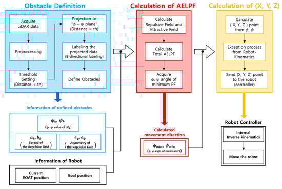
Figure 2.
Flowchart of proposed real-time collision avoidance system.
2.1. Obstacle Definition
Let the Z value of the i-th point data from the LiDAR, after being converted to coordinates, be denoted as , and let the Z value of the current robot’s EOAT be denoted as . If , the corresponding LiDAR data are considered as part of the ground plane or noise and are subsequently removed (Steps (1)∼(2) of Figure 3). After this preprocessing, all subsequent procedures are conducted in the LiDAR coordinate system, represented by the axes (vertical angle), (horizontal angle), and distance. This approach is motivated by the fact that when the movement of robots primarily performing rotational motions or vehicles adjusting their steering angles aligns with the coordinate system of LiDAR data, collision avoidance algorithms can be designed more intuitively and efficiently. For a clearer understanding, refer to Figure 4, which represents the LiDAR data in two different coordinate systems.
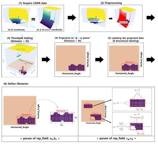
Figure 3.
Flow visualization of obstacle defining.
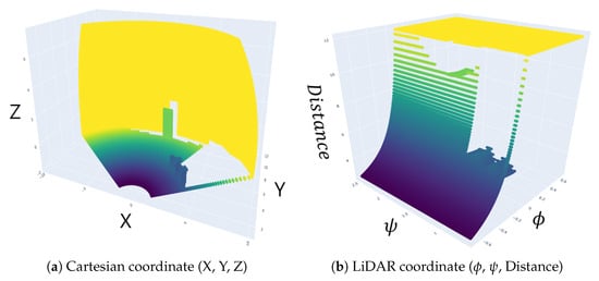
Figure 4.
Representation of LiDAR data in two coordinate systems.
After completing the preprocessing of LiDAR data, a specific threshold () is set to filter the data. Only the data within the threshold, which is directly relevant to collision avoidance, are passed to the next stage. This step focuses on nearby obstacles that have an immediate impact on the robot’s movement while removing noise caused by distant objects. Additionally, it reduces unnecessary computations when calculating the AELPF, enabling the real-time update of the AELPF for collision avoidance (Steps (3)∼(4) of Figure 3).
Data points representing nearby obstacles with a distance value smaller than the threshold () are projected onto a plane where . This projection transforms the 3D data into a 2D representation on the threshold plane. The resulting plane is treated as a single image, and eight-directional labeling, commonly used in computer vision, is applied to define individual obstacles [15]. Each pixel in this “image” corresponds to a projected data point, and the eight-directional connectivity is used to group and identify obstacle regions. Using the eight-directional labeling, obstacles are defined based on their spatial relationships, ensuring that neighboring data points are grouped together to form distinct obstacle clusters.
2.2. Calculation of AELPF
The flowchart for the calculation of the AELPF is illustrated in Figure 5. The main framework of the AELPF algorithm, as depicted in this figure, does not differ significantly from the Conventional Potential Field [16]. Both share the fundamental structure of ensuring that a moving object reaches its goal safely, without colliding with obstacles or entering dangerous areas through an Artificial Potential Field composed of an attractive field and a repulsive field. The attractive field pulls the moving object toward the goal point, guiding it to the target location, while the repulsive field pushes the object away from obstacles or regions it should avoid, ensuring the object’s safety during motion. Figure 6 illustrates examples of these fields in a Conventional Potential Field.
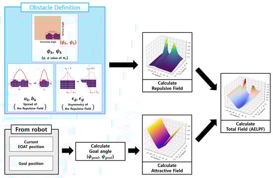
Figure 5.
Flowchart of calculation of AELPF.
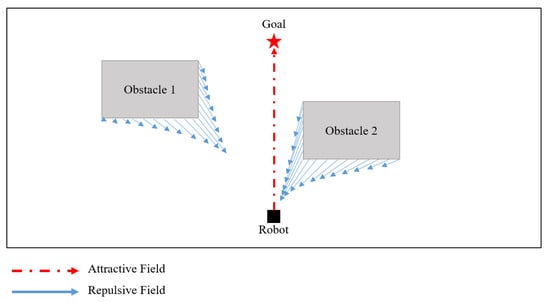
Figure 6.
Attractive field and repulsive field in Conventional Potential Field.
However, when a robot moves toward a specific location and encounters obstacles along its path, it must consider collision avoidance in a three-dimensional space, accounting for both vertical and horizontal environmental factors. Unlike scenarios where global environmental information is available, the robot relies on local environmental data obtained through LiDAR to avoid collisions in its forward path. This reliance highlights the limitations of the Conventional Potential Field, as it cannot fully account for the dynamic, 3D environment. To address these limitations, the attractive and repulsive fields were constructed as follows.
2.2.1. Target Attractive Field
In order for the attractive field of the AELPF to be generated in the LiDAR coordinate system, the robot’s direction of movement needs to be defined in terms of angles. The vertical and horizontal angles, and , which are the data format of the LiDAR, are used to define the robot’s direction of movement, thereby establishing the attractive field.
The attractive field is defined as
where is a scaling factor that adjusts the magnitude of the attractive field and determines the strength of the attraction toward the goal direction. A larger increases the attraction, causing the robot to move more rapidly toward the goal. However, if is too large, it may lead to excessive movement or oscillations near the goal, potentially destabilizing the system. On the other hand, a smaller reduces the attraction strength, resulting in smoother, more stable motion but may increase the time required to reach the goal.
Therefore, the appropriate value of should be determined through several simulations. And the subscripts i and j denote the indices of the vertical angle and the horizontal angle data segments, respectively. This distinction accounts for the possibility that the horizontal and vertical angular resolutions may differ. This formulation represents the Euclidean distance in angular space between the goal direction and the current sensor reading , scaled by . By minimizing this value, the system generates a movement trajectory that guides the robot toward the target orientation.
2.2.2. Obstacle Repulsive Field
In the AELPF framework, the Obstacle Repulsive Field serves to generate a potential that pushes the robot away from obstacles detected by the LiDAR sensor. This field influences the robot’s path based on angular deviations and the relative motion between the robot’s end-effector and the obstacles. Similar to the attractive field described in Section 2.2.1, the repulsive field is defined in terms of angles within the LiDAR coordinate system. The repulsive field can be expressed as
where n represents the number of obstacles detected by the LiDAR, is the strength of the repulsive potential for the k-th obstacle, and and represent the angular deviations in the and directions, respectively.
The magnitude of the repulsive potential depends on the distance to the obstacle and the relative velocity. The equation for is given by
where is the distance to the k-th obstacle, is the maximum effective distance for the repulsive field, is the relative velocity between the end-effector and the k-th obstacle, is the maximum relative velocity, and is a weighting coefficient that adjusts the influence of the relative velocity. To ensure effective obstacle avoidance, must be set such that the ellipsoidal repulsive field fully covers the area around the obstacle within its effective range. This ensures that the repulsive potential can adequately influence the robot’s path when obstacles are nearby or moving towards the robot.
The angular deviations and account for the repulsive effects in the (vertical) and (horizontal) angular directions, respectively. These deviations are computed using the following equations:
where and are the angles of the current LiDAR measurement point, while and are the angles corresponding to the k-th obstacle. And the parameters and control the spread of the repulsive field in the and directions, respectively.
The parameters and are defined to be proportional to the height and width of the bounding boxes of the obstacles, respectively, as illustrated in Figure 7 and identified in Step (5) of Figure 3. Also, and are calculated as
where is a proportional constant that should be determined through several simulations.
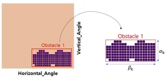
Figure 7.
Definition of and .
In (4), the coefficients and adjust the field asymmetry based on the hyperbolic tangent function. The extent to which the center of a recognized obstacle deviates from the center of its bounding box is defined as the value of and . It can be expressed as follows:
where the term represents the -component of the center point of the k-th recognized obstacle, and represents the -component of the center point of the k-th recognized obstacle.
In the case of Obstacle 1, as illustrated in Figure 8, as the center point of Obstacle 1 () coincides with the center point of the bounding box for Obstacle 1 (), the asymmetry of the repulsive field is zero, implying that both and are equal to zero. Similarly, in the case of Obstacle 2, as the center point of Obstacle 2 () is located in the positive directions of and relative to the center point of the bounding box for Obstacle 2 (), both and will have positive values.
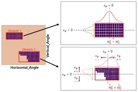
Figure 8.
Definition of and .
The repulsive field effectively repels the robot from obstacles based on both distance and angular deviation. The elliptical structure defined by and allows the repulsive field to dynamically adapt to obstacle shapes and orientations. Additionally, the inclusion of relative velocity in ensures that the field responds more strongly to fast-approaching obstacles, enhancing safety in dynamic environments. This formulation enables the AELPF method to provide a balanced and adaptive repulsive force, helping the robot navigate safely while maintaining responsiveness to its surroundings. And Figure 9 shows a graph of attractive and repulsive field of AELPF.
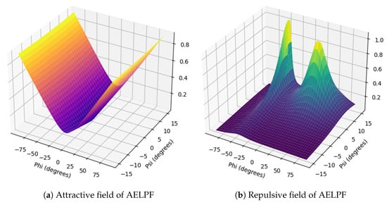
Figure 9.
Visualization of the attractive and repulsive field in AELPF.
2.2.3. Integration of Attractive Field and Repulsive Field
In the AELPF framework, the final potential field is derived by integrating the attractive field and the repulsive field. This integration allows the robot to navigate safely toward its target while avoiding obstacles dynamically detected in the environment. The combined potential field is computed as follows:
where is the attractive field guiding the robot toward the goal (see Section 2.2.1), and is the repulsive field pushing the robot away from obstacles (see Section 2.2.2).
The attractive field is designed to minimize the angular distance between the robot’s current direction and the goal direction, as defined in Equation (1). This field exerts a pulling effect, encouraging the robot to move efficiently toward its target. In contrast, the repulsive field defined in Equation (2) creates a pushing effect, ensuring that the robot maintains a safe distance from obstacles detected by the LiDAR sensor. The balance between these two fields is crucial for achieving smooth and safe motion. When the robot is far from any obstacle, the repulsive field has minimal influence, allowing the attractive field to dominate and guide the robot toward its goal. As the robot approaches an obstacle, the repulsive field increases significantly, counteracting the attractive field and diverting the robot’s path to avoid collisions.
To achieve real-time responsiveness, the potential fields are recalculated continuously as new LiDAR data are received. At each iteration, the robot determines the direction with the lowest total potential and adjusts its trajectory accordingly. This process ensures that the robot dynamically responds to changes in the environment, such as moving obstacles or newly detected objects.
The weighting parameters for the attractive field and for the repulsive field play a key role in this integration. If is too large, the robot may prioritize reaching the goal over avoiding obstacles, leading to potential collisions. Conversely, if is too large, the robot may become overly cautious and fail to make efficient progress toward the goal. Therefore, these parameters must be carefully tuned through simulations to achieve a balance that ensures both safety and efficiency.
In addition to parameter tuning, the asymmetry coefficients and further enhance the flexibility of the repulsive field. By adjusting the asymmetry based on the relative positions of obstacles, the robot can generate more sophisticated avoidance paths, particularly in environments where obstacles are not uniformly distributed.
Figure 10 provides an illustration of the integrated potential field in a dynamic environment. The figure shows how the attractive field pulls the robot toward the goal while the repulsive field pushes it away from nearby obstacles. The resulting path demonstrates the robot’s ability to navigate safely and efficiently through complex environments.
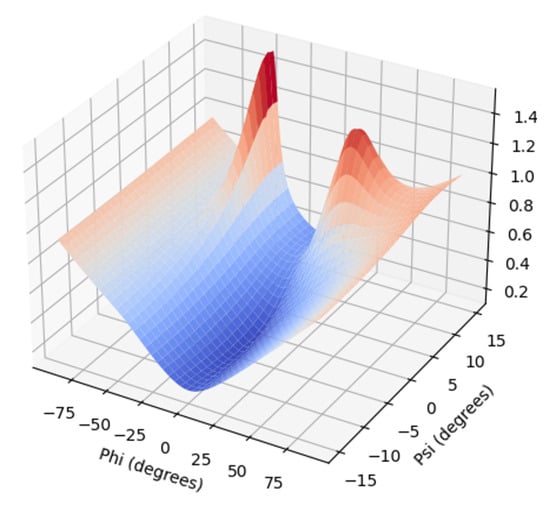
Figure 10.
Visualization of the total field of AELPF.
2.3. Calculation of (X,Y,Z) Point from AELPF
The direction corresponding to the lowest AELPF value in terms of horizontal and vertical angles, as determined in Section 2.2.3, is used to estimate the position the robot will occupy approximately 8 ms later, considering its current velocity. As a result, this position represents where the robot can avoid obstacles. This enables real-time path adjustments, ensuring a smooth and collision-free avoidance trajectory.
The integrated potential field approach in the AELPF provides a robust collision avoidance system that can adapt to real-time changes. By leveraging both the attractive and repulsive fields in the LiDAR coordinate system, the method ensures that the robot maintains a clear path toward its goal while dynamically avoiding obstacles. This approach offers a significant improvement over conventional methods, especially in environments where robots and human workers collaborate closely.
In addition, the AELPF employs an Asymmetric Elliptical Repulsive Field to avoid obstacles, which applies differential weighting in vertical and horizontal directions to adjust repulsive forces based on obstacle shape and relative position. This asymmetric field generation is particularly effective in providing alternative escape routes when obstacles significantly impact the robot’s movement direction, overcoming the limitations of traditional isotropic repulsive fields that are prone to local minima.
3. Experiments
3.1. Experimental Environments
In this experiment, the obstacle avoidance performance of the AELPF algorithm was compared with the VFH (Vector Field Histogram) algorithm [17] and the FGM (Follow the Gap Method) algorithm [18]. These two methods are widely used path planning algorithms in industrial environments and have been extensively applied in industrial and mobile robots, making them standard approaches for real-time obstacle avoidance.
Therefore, one of the primary objectives of this study is to verify the extent to which the AELPF improves performance compared to these industry-standard techniques. To achieve this, we designed two experimental scenarios to evaluate the algorithms under different obstacle conditions.
As shown in Figure 11a, Scenario 1 consists of a robot and two stationary obstacles of different sizes and heights, positioned in front of the robot along with predefined start and goal positions. In Scenario 2, shown in Figure 11b, one of the obstacles (100 cm in height) moves toward the Goal Point, introducing a dynamic element to the experiment. The LiDAR sensor, mounted on the EOAT of the robot, was used to acquire real-time obstacle position and direction information.
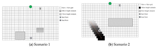
Figure 11.
Robot and obstacle positions for each scenario.
The data processing environment was configured on an external computer, and its specifications are listed in Table 1. This setup handled tasks such as LiDAR data collection, point cloud transformation into the world coordinate system, and the execution of obstacle avoidance algorithms (VFH, FGM, and AELPF).

Table 1.
External computer specifications.
The LiDAR used in the experiment was Velodyne’s VLP-16 model, which has specifications as listed in Table 2. The robot was the S6-1835 model from HYRobotics, featuring six degrees of freedom, with specifications presented in Figure 12 [19]. The robot control library provided by the controller manufacturer was utilized for real-time position updates of all robot axes (A1∼A6). This enabled effective joint error dynamics control. Control commands for each axis were calculated to ensure that the maximum allowable angular velocity, based on the manufacturer’s motor specifications, was not exceeded.
Table 2.
VLP-16 Specifications.
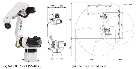
Figure 12.
Robots and specifications used in the experiments.
3.2. Experimental Results
3.2.1. Simulation
The algorithms compared in the experiment, VFH and FGM, are primarily designed to operate in a planar coordinate system, with limited capabilities for obstacle avoidance in the z-axis direction. The VFH algorithm generates an angle-based vector field to steer clear of nearby obstacles, while the FGM algorithm tracks gaps between obstacles along the path toward the target destination. However, both algorithms exhibit limited ability to avoid obstacles along the z-axis in a 3D environment. In contrast, the AELPF algorithm proposed in this study operates effectively in three-dimensional space. It is capable of generating paths that consider not only the horizontal plane but also the z-axis, thereby providing effective navigation even in complex 3D obstacle environments.
The results of simulation (see Figure 13) demonstrated that the AELPF algorithm outperformed the VFH and FGM algorithms, particularly in its ability to avoid obstacles precisely in three-dimensional environments. The VFH and FGM algorithms, which primarily operate in a planar space, were unable to generate effective paths when obstacles were located along the z-axis. Both algorithms tended to approach or even collide with obstacles in the z-direction. However, the AELPF algorithm addressed this issue, successfully avoiding obstacles located along the z-axis and generating paths toward the target destination.
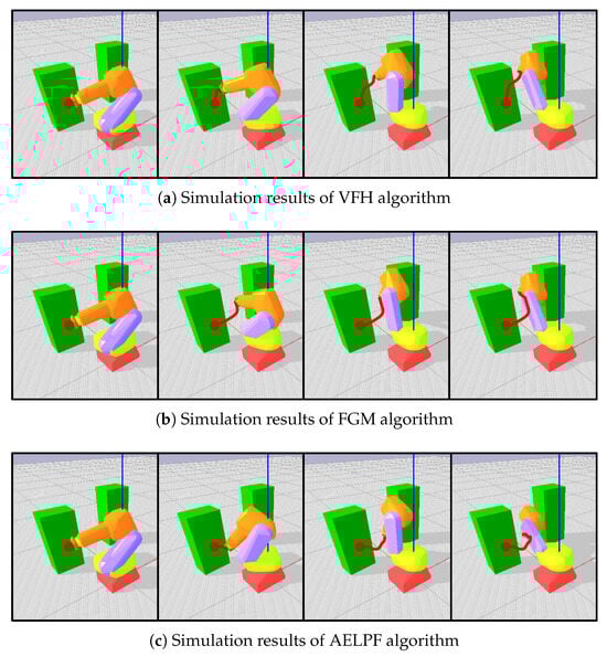
Figure 13.
Simulation results.
In particular, the AELPF algorithm showed a significant advantage in obstacle avoidance along the z-axis compared to the other two algorithms. While the VFH and FGM algorithms had limited obstacle avoidance capabilities in 3D space, often bringing the path too close to obstacles, the AELPF algorithm effectively incorporated real-time feedback from obstacle positions, allowing for efficient avoidance of obstacles in the z-direction and precise path corrections toward the target destination. As a result, the AELPF algorithm demonstrated superior performance in complex scenarios requiring obstacle avoidance in 3D environments.
3.2.2. Physical Experiments
The experimental environment consists of a Velodyne VLP-16, an external computer, and a robot controller, which has specifications as listed in Table 3. The Velodyne VLP-16 LiDAR consists of a LiDAR sensor that generates 3D point clouds and an interface box module that transmits data via an Ethernet port. The data are sent to a laptop through the Ethernet connection. The robot’s movement coordinates, calculated by the AELPF algorithm on the PC, are transmitted to the robot controller, CP505/A, via the Ethernet connection (see Figure 14). Upon receiving the movement coordinates, the robot moves to the specified position under the control of the KEBA robot control system and updates the EOAT position in real time.
Table 3.
Specifications of experimental equipment.
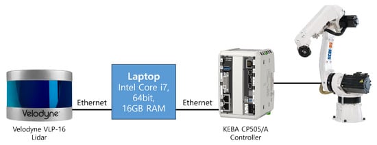
Figure 14.
Sensor and controller configuration.
In this section, a physical experiment was conducted to verify the performance of the AELPF algorithm in a real-world environment. The experimental setup was designed to be identical to the simulation environment, where an industrial robot was tasked with navigating toward a target while avoiding surrounding obstacles.
In Experimental Scenario 1, as shown in Figure 15, the experimental results demonstrated that the VFH and FGM algorithms exhibit poor obstacle avoidance performance in a 3D environment, similar to the simulation results. In particular, as observed in Figure 15c, the VFH algorithm frequently collided with obstacles in areas with abrupt environmental changes, such as edges and boundaries. This is because the VFH algorithm represents obstacle information using a histogram based on grid cells, which limits its ability to smoothly handle obstacle boundaries, ultimately leading to collisions.
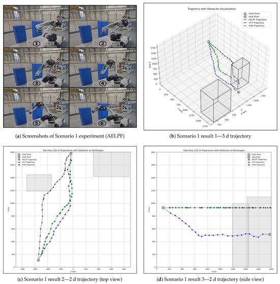
Figure 15.
Scenario 1 results of AELPF.
In Experimental Scenario 2, as shown in Figure 16c, the VFH algorithm tended to move away from the Goal Point while avoiding collisions with moving obstacles. However, once the obstacles stopped, the algorithm resumed moving toward the Goal Point, resulting in an overall longer path. Additionally, the FGM algorithm, when detecting moving obstacles, exhibited a tendency to deviate further from the Goal Point as the gap between obstacles widened.
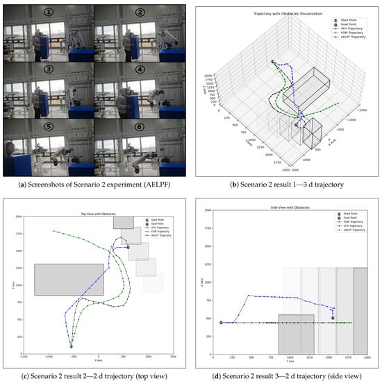
Figure 16.
Scenario 2 results of AELPF.
On the other hand, the AELPF algorithm effectively utilized real-time feedback from the LiDAR sensor to accurately recognize the position of obstacles and generate smooth avoidance paths even in the z-axis direction. As a result, it successfully maintained a stable avoidance path and reached the Goal Point without collisions.
As seen in the Table 4, the average computation speed of the AELPF algorithm was measured at 224 ms, whereas the VFH algorithm recorded 50 ms and the FGM algorithm 22 ms, demonstrating relatively faster processing times. The VFH and FGM algorithms utilize a single-channel LiDAR for obstacle avoidance in a 2D plane, resulting in lower computational complexity and faster speeds. In contrast, the AELPF algorithm employs a 16-channel LiDAR, enabling precise obstacle avoidance in a 3D environment, which distinguishes it from the other methods.
Table 4.
Comparison of experimental results by algorithm.
Considering the scenario where all algorithms use a 16-channel LiDAR, the computation speed of the FGM algorithm increases to 352 ms, and the VFH algorithm to 800 ms, whereas the AELPF algorithm remains at 224 ms. This indicates that the AELPF algorithm is approximately 3.57 times faster than the VFH algorithm and 1.57 times faster than the FGM algorithm. These results confirm that the AELPF is an efficient avoidance algorithm capable of handling high computational loads while maintaining real-time performance.
4. Conclusions
This paper proposes a new algorithm, the AELPF algorithm, for efficient and safe obstacle avoidance in industrial robots. The experimental results show that compared to existing obstacle avoidance algorithms, VFH and FGM, the AELPF algorithm significantly improves obstacle avoidance performance in a 3D environment, demonstrating the ability to avoid obstacles more precisely. In particular, there was a notable difference in obstacle avoidance ability along the z-axis.
The findings of this study confirm that the AELPF algorithm can generate more precise and effective obstacle avoidance paths in a 3D environment, showing potential for flexible adaptation to various obstacle avoidance scenarios. Furthermore, due to these characteristics, it is expected that the AELPF algorithm could be effectively applied in diverse fields such as autonomous robots and drones handling complex 3D obstacle environments.
Future research will focus on enhancing the algorithm’s performance by considering various speed variations between the EOAT and complex obstacle environments. Additionally, we plan to explore methods for incorporating not only the EOAT but also other dynamic elements of industrial robots (e.g., joints, body, etc.) into the avoidance algorithm. Furthermore, we will investigate the feasibility of applying the AELPF algorithm to humanoid robots, taking into account articulated structures and dynamic movements. By optimizing obstacle avoidance strategies for humanoid robots, our goal is to improve adaptability in human–robot collaboration environments.
Additionally, we plan to conduct research on a multi-agent approach aimed at developing techniques for dynamically generating optimal paths to enable efficient collaboration between multiple robots in industrial environments. Furthermore, we will optimize the hyperparameters of the AELPF algorithm through reinforcement learning or genetic algorithms to enhance the algorithm’s stability and achieve more precise and reliable avoidance performance. Moreover, in future research, we will explore how to apply a more structured real-time control framework [20,21] to the AELPF, aiming to improve its responsiveness and adaptability in practical settings.
Author Contributions
Conceptualization, E.-G.H., D.-M.S. and T.-K.K.; Data curation, E.-G.H. and D.-M.S.; Formal analysis, T.-K.K. and H.-J.Y.; Methodology, E.-G.H. and D.-M.S.; Software, E.-G.H., D.-M.S., J.-S.L. and H.-Y.K.; Validation, S.-Y.K. and H.-J.Y.; Writing—original draft, E.-G.H. and D.-M.S.; Writing—review and editing, T.-K.K. and H.-J.Y. All authors have read and agreed to the published version of the manuscript.
Funding
This research received no external funding.
Data Availability Statement
Data are contained within the article.
Conflicts of Interest
Authors Ean-Gyu Han, Dong-Min Seo, Shin-Yeob Kang and Ho-Joon Yang were employed by the company Hanyang Robotics. The remaining authors declare that the research was conducted in the absence of any commercial or financial relationships that could be construed as a potential conflict of interest.
References
- Islam, R.U.; Iqbal, J.; Manzoor, S.; Khalid, A.; Khan, S. An autonomous image-guided robotic system simulating industrial applications. In Proceedings of the 2012 7th International Conference on System of Systems Engineering (SoSE), Genova, Italy, 16–19 July 2012; pp. 344–349. [Google Scholar] [CrossRef]
- Acemoglu, D.; Restrepo, P. Industrial Robots, Workers’ Safety, and Health. Natl. Bur. Econ. Res. 2022, 78, 102205. [Google Scholar] [CrossRef]
- Płaczek, M.; Piszczek, Ł. The method for tests of emergency stopping of industrial robots. Model. Inżynierskie 2018, 38, 60–67. [Google Scholar]
- Fryman, J. Updating the industrial robot safety standard. In Proceedings of the ISR/Robotik 2014; 41st International Symposium on Robotics, Munich, Germany, 2–3 June 2014; VDE: Berlin, Germany, 2014; pp. 1–4. [Google Scholar]
- Bott, B.; Weingarten, R. Safety in Human-Robot Interaction: A Review. Hum.-Centric Comput. Inf. Sci. 2015, 5, 1–15. [Google Scholar]
- Franz, M.; Reinders, D. A Safety System for Collaborative Robots. Int. J. Adv. Robot. Syst. 2017, 14, 1–10. [Google Scholar]
- Park, J.; Lee, S. Real-time Collision Avoidance for Human-Robot Collaboration in Manufacturing. Robot. Comput.-Integr. Manuf. 2020, 61, 1–12. [Google Scholar]
- Alonso, F.; El Saddik, A. A Survey on Safety in Human-Robot Collaboration: Current Issues and Future Directions. J. Robot. 2018, 2018, 1–13. [Google Scholar]
- Robla-Gómez, S.; Becerra, V.M.; Llata, J.R.; Gonzalez-Sarabia, E.; Torre-Ferrero, C.; Perez-Oria, J. Working together: A review on safe human-robot collaboration in industrial environments. IEEE Access 2017, 5, 26754–26773. [Google Scholar] [CrossRef]
- Du, J.; Cai, C.; Zhang, P.; Tan, J. Path planning method of robot arm based on improved RRT* algorithm. In Proceedings of the 2022 5th International Conference on Robotics, Control and Automation Engineering (RCAE), Changchun, China, 28–30 October 2022; IEEE: Phoenix, AZ, USA, 2022; pp. 236–241. [Google Scholar]
- Kobayashi, M.; Motoi, N. Local path planning: Dynamic window approach with virtual manipulators considering dynamic obstacles. IEEE Access 2022, 10, 17018–17029. [Google Scholar] [CrossRef]
- Feng, S.; Sebastian, B.; Ben-Tzvi, P. A collision avoidance method based on deep reinforcement learning. Robotics 2021, 10, 73. [Google Scholar] [CrossRef]
- Hu, J.; Yang, X.; Wang, W.; Wei, P.; Ying, L.; Liu, Y. Obstacle avoidance for uas in continuous action space using deep reinforcement learning. IEEE Access 2022, 10, 90623–90634. [Google Scholar] [CrossRef]
- Cho, J.H.; Pae, D.S.; Lim, M.T.; Kang, T.K. A Real-Time Obstacle Avoidance Method for Autonomous Vehicles Using an Obstacle-Dependent Gaussian Potential Field. J. Adv. Transp. 2018, 2018, 5041401. [Google Scholar] [CrossRef]
- He, L.; Chao, Y.; Suzuki, K. A run-based two-scan labeling algorithm. IEEE Trans. Image Process. 2008, 17, 749–756. [Google Scholar] [PubMed]
- Khatib, O. Real-time obstacle avoidance for manipulators and mobile robots. Int. J. Robot. Res. 1986, 5, 90–98. [Google Scholar] [CrossRef]
- Borenstein, J.; Koren, Y. The vector field histogram-fast obstacle avoidance for mobile robots. IEEE Trans. Robot. Autom. 1991, 7, 278–288. [Google Scholar] [CrossRef]
- Sezer, V.; Gokasan, M. A novel obstacle avoidance algorithm: “Follow the Gap Method”. Robot. Auton. Syst. 2012, 60, 1123–1134. [Google Scholar] [CrossRef]
- HYrobotics Co., Ltd. HYrobotics Official Website. 2025. Available online: https://www.hyrobot.com (accessed on 10 February 2025).
- Zhao, J.; Wang, Z.; Lv, Y.; Na, J.; Liu, C.; Zhao, Z. Data-Driven Learning for H∞ Control of Adaptive Cruise Control Systems. IEEE Trans. Veh. Technol. 2024, 73, 18348–18362. [Google Scholar] [CrossRef]
- Jleilaty, S.; Ammounah, A.; Abdulmalek, G.; Nouveliere, L.; Su, H.; Alfayad, S. Distributed real-time control architecture for electrohydraulic humanoid robots. Robot. Intell. Autom. 2024, 44, 607–620. [Google Scholar] [CrossRef]
Disclaimer/Publisher’s Note: The statements, opinions and data contained in all publications are solely those of the individual author(s) and contributor(s) and not of MDPI and/or the editor(s). MDPI and/or the editor(s) disclaim responsibility for any injury to people or property resulting from any ideas, methods, instructions or products referred to in the content. |
© 2025 by the authors. Licensee MDPI, Basel, Switzerland. This article is an open access article distributed under the terms and conditions of the Creative Commons Attribution (CC BY) license (https://creativecommons.org/licenses/by/4.0/).