Optimal Control Model of Electromagnetic Interference and Filter Design in Motor Drive System

Abstract

Electromagnetic interference (EMI) is a key problem in the design of electric vehicle motor drive systems. Based on the system composition and conducted EMI mechanism, an equivalent circuit model including a motor, inverter, cable, and battery is established, and an optimized double closed-loop control strategy is proposed. Through the joint simulation platform of Simulink and Simplorer, the conduction EMI prediction model of a motor drive system is constructed. On this basis, a filter design method based on Π-type topology is proposed based on the 6 dB safety margin of reducing the interference limit. The simulation results show that the designed filter significantly suppresses the conducted EMI in the frequency band from 150 kHz to 30 MHz, and the interference peak is reduced by approximately 40 dBμV. The effectiveness of the model and filter is verified by experimental tests, and the electromagnetic compatibility (EMC) performance of the system is improved, which provides theoretical support and an engineering reference for the high-frequency interference suppression of the motor drive system.

1. Introduction

The core system that distinguishes electric vehicles from [1] traditional internal combustion engine vehicles is the motor drive system [2]. During vehicle operation, the motor drive system continuously exchanges energy using high-power devices in the drive system, such as insulated gate bipolar transistors (IGBTs), silicon carbide (SiC), and gallium nitride (GaN).

Components [3,4] frequently switch, leading to significant voltage (du/dt) and current (di/dt) rate changes. These changes are the primary sources of electromagnetic interference (EMI) during vehicle operation [5]. EMI can be classified into conducted interference and radiated interference [6]. Radiated interference is generated according to antenna principles, while conducted EMI forms closed loops within the circuit, radiating electromagnetic waves outward. Therefore, EMI research mainly focuses on conducted electromagnetic interference [7,8]. According to the GB/T 33012.1-2016 standard [9] “Electromagnetic Compatibility Terminology for Road Vehicles”, vehicle electromagnetic compatibility is defined as “the ability of the vehicle, electrical/electronic systems, or components to function normally within the vehicle’s electromagnetic environment without affecting the normal operation of other vehicles, systems, or components [10]”. Conducted EMI propagates to the ground and transmission lines through parasitic capacitances, affecting the vehicle’s operation and interfering with nearby components [11].

In 2013, Guo, YJ proposed a systematic method to analyze conducted electromagnetic interference (EMI) in electric vehicle (EV) drive systems. By establishing equivalent models from power devices to the entire system, the study examined the inverter, battery, and motor as the primary sources and propagation paths of interference, with simulation and experimental verification confirming the model’s accuracy [12]. In 2015, Yang, YM introduced a common-mode electromagnetic interference (CM EMI) prediction model, which used equivalent circuit modeling to represent various components in electric vehicles’ motor drive systems. The model’s effectiveness was verified experimentally in the frequency range of 150 kHz to 30 MHz [13]. In 2020, Duan, Z·L proposed a new analytical method for predicting conducted EMI in silicon carbide (SiC) motor drive systems. By considering the fast switching of SiC devices, parasitic parameters of power modules, and other circuit parameters, this method accurately predicted EMI in the frequency range of 150 kHz to 30 MHz for SiC drive systems in electric vehicles, improving the prediction accuracy of differential-mode (DM) EMI in the high-frequency range [14]. In 2020, Yang, M presented a motor drive system based on gallium nitride (GaN) power devices, addressing electrical resonance caused by the LC filter and stator inductance with a sine-wave filter and an undamped variable delay method. The system effectively reduced electromagnetic interference (EMI) using spread spectrum modulation techniques, and experimental results validated the effectiveness of the design [15].

Previous studies typically used equivalent circuit modeling and frequency domain analysis methods to predict EMI. However, this study improves accuracy through a co-simulation approach combining Simulink and Simplorer, a dual-loop control strategy, and a filter design method based on a 6 dB safety margin. To address the EMI issue, this paper establishes a system-level equivalent circuit model of the motor drive system in Simplorer based on the system’s composition and working principle [16,17,18,19,20]. The control model in the existing predictive model is optimized by adopting a speed and current dual-loop control strategy, ensuring more accurate simulation results and laying the foundation for subsequent EMI filter design. The motor electromagnetic interference is studied through a Simulink–Simplorer co-simulation. Based on the simulation results, a filter topology design method is proposed, and its feasibility is validated through experiments.

2. Motor Drive System Conducted EMI Prediction Mode

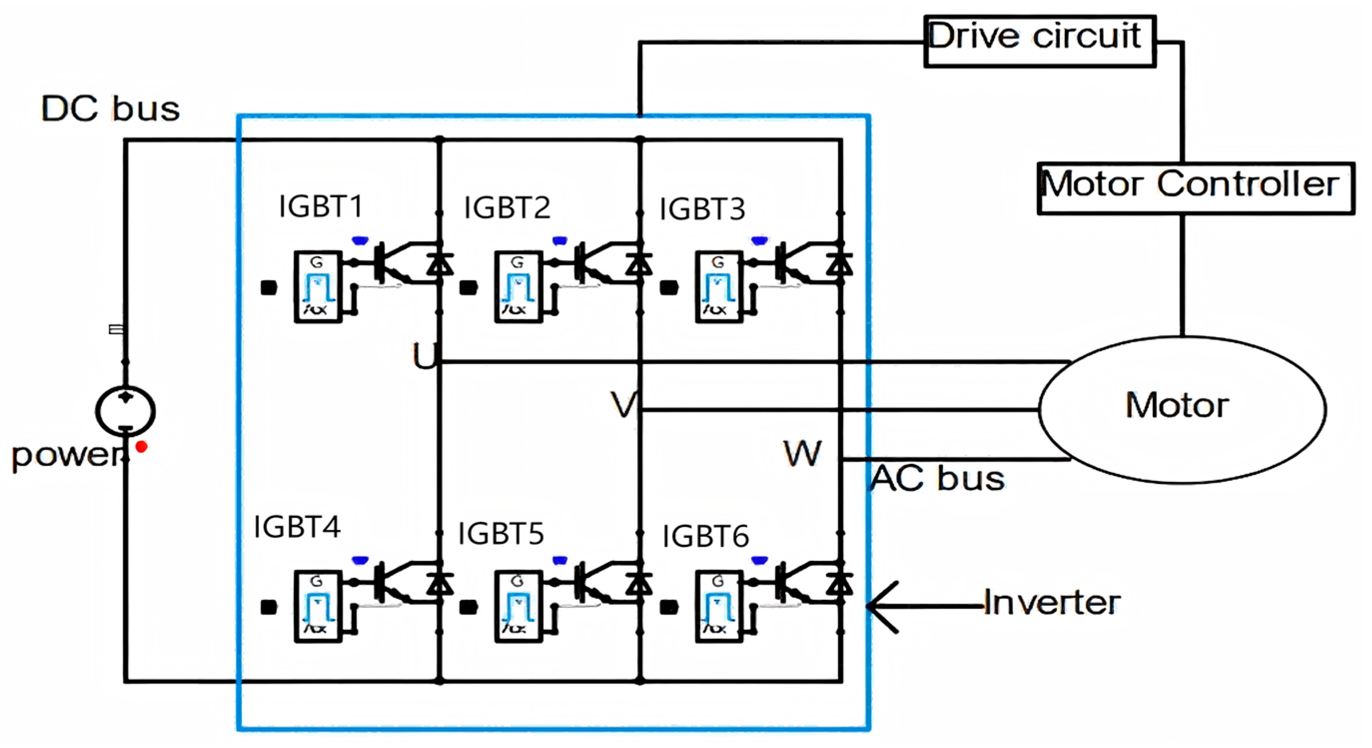
2.1. Composition and Working Principle of the Motor Drive System

When analyzing the electromagnetic interference of the electric drive system of electric vehicles, the motor drive system is usually regarded as a battery and a DC bus, an inverter, an AC bus, and a motor composed of five parts. The topology is shown in Figure 1, in which the battery management system, drive circuit, and motor controller are the control circuits of each unit of the system.

The output voltage of the battery is monitored and protected by the battery management system (BMS), and the power output of the vehicle is coordinated by the motor controller and the inverter. Dynamic control is achieved by adjusting the PWM duty cycle and current feedback. The battery’s power output fluctuates depending on the vehicle’s operating conditions. The inverter plays a crucial role in converting the battery’s direct current (DC) into alternating current (AC), which is necessary for the operation of the permanent magnet synchronous motor (PMSM). The inverter uses a three-phase two-level bridge circuit, and its switching devices are controlled by a drive circuit. This drive circuit receives feedback signals from the motor controller, which guide the switching of the devices to precisely control motor speed and torque.

The DC bus and AC bus act as connection bridges between different components of the drive system. To enhance the system’s electromagnetic compatibility (EMC), these buses are often shielded. The DC bus links the battery to the inverter, while the AC bus connects the inverter to the motor. The motor is the key component of the drive system, facilitating the conversion of electrical energy into mechanical energy for vehicle propulsion.

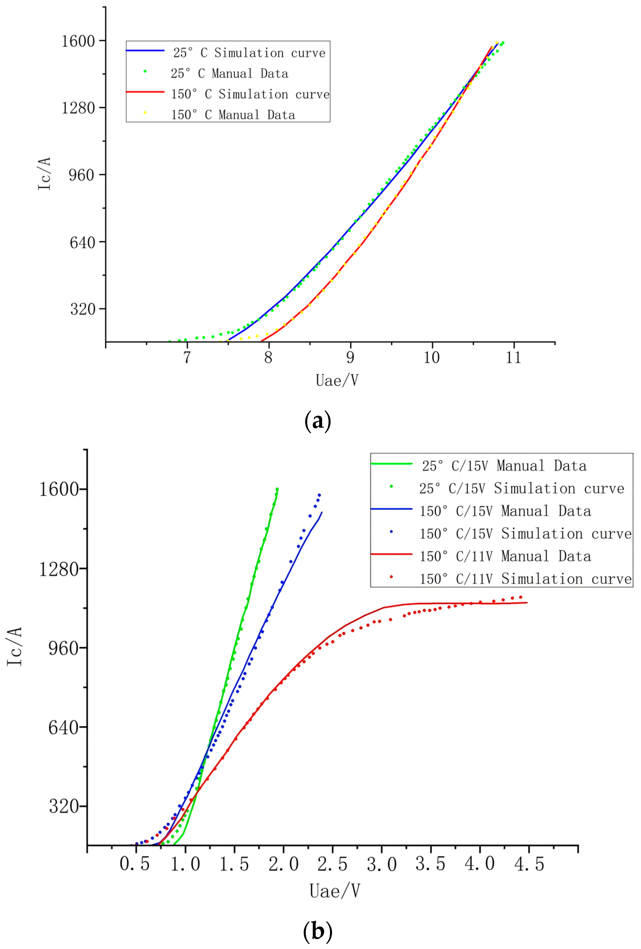
2.2. IGBT Model

In the electric drive system studied in this paper, the selected switching device is Infineon IGBT model FS820RO8A6P2B. The model is established by using the dynamic model window of the power equipment in the simplifier. According to the parameters and characteristic curves in the data file, the advanced dynamic model of IGBT is established according to the process of Figure 2. Infineon’s data manual has given the static characteristic curve of IGBT, as shown in Figure 3.

According to the data manual, the parameters are imported in turn, as shown in

Table 1. IGBT data parameters.

Category	Parameter	Value	Unit	Category	Parameter	Value	Unit
Basic Electrical	Collector–Emitter Voltage (${\mathrm{V}}_{\mathrm{C}\mathrm{E}}$)	400	V	Capacitance	Input Capacitance (${\mathrm{C}}_{\mathrm{i}\mathrm{e}\mathrm{s}}$)	80	nF
	Collector Current (${\mathrm{I}}_{\mathrm{C}}$)	450	A		Miller Capacitance (${\mathrm{C}}_{\mathrm{r}\mathrm{e}\mathrm{s}}$)	0.3	nF
	Reference Temperature	150	°C	Resistance	Gate Resistance (${\mathrm{R}}_{\mathrm{G}}$)	0.7	Ω
Gate Drive	Gate-On Voltage (${\mathrm{V}}_{\mathrm{G}\mathrm{E}}\left(\mathrm{o}\mathrm{n}\right)$)	15	V		Collector–Emitter Resistance (${\mathrm{R}}_{\mathrm{C}\mathrm{E}}$)	35	mΩ
	Gate-Off Voltage (${\mathrm{V}}_{\mathrm{G}\mathrm{E}}\left(\mathrm{o}\mathrm{f}\mathrm{f}\right)$)	8	V		External Gate-On Resistance (${\mathrm{R}}_{\mathrm{G}\left(\mathrm{o}\mathrm{n}\right)}$)	2.4	Ω
Breakdown Characteristics	Breakdown Voltage (${\mathrm{V}}_{\mathrm{B}\mathrm{R}}$)	750	V		External Gate-Off Resistance (${\mathrm{R}}_{\mathrm{G}\left(\mathrm{o}\mathrm{f}\mathrm{f}\right)}$)	5.1	Ω
	Breakdown Current (${\mathrm{I}}_{\mathrm{B}\mathrm{R}}$)	1650	A	Inductance	Collector–Emitter Stray Inductance (${\mathrm{L}}_{\mathrm{C}\mathrm{E}}$)	4	nH
	Breakdown Temperature	175	°C		Cascaded Modules’ Stray Inductance (${\mathrm{L}}_{\mathrm{c}\mathrm{a}\mathrm{s}\mathrm{c}\mathrm{a}\mathrm{d}\mathrm{e}}$)	20	nH

.

The IGBT static characteristic measurement circuit is shown in Figure 4. In the Simplorer simulation software (Ansys Electronics Desktop 2022), the collector–emitter voltage $V_{ce}$ is scanned parametrically by fixing the gate–emitter voltage $V_{ge}$ so as to obtain the output characteristic curve of IGBT, as shown in Figure 5a. Then, the collector–emitter voltage $V_{ce}$ is fixed, and the gate–emitter voltage $V_{ge}$ is parametrically scanned to obtain the IGBT transfer characteristic curve, as shown in Figure 5b. By comparing Figure 3 and Figure 5, it can be seen that the static characteristic curve of IGBT obtained by simulation is consistent with that in the data manual, which verifies that the established simulation model can accurately simulate the static characteristics of actual IGBT devices.

By using the curve fitting method provided by the software and inputting the data table parameters, the transfer characteristic curve and the output characteristic fitting curve of the gate opening voltage and the collector opening current can be obtained, as shown in Figure 5. Figure 5a is the fitting result of transfer characteristics. The blue solid line in the figure is the fitted transfer characteristic curve at 25 °C, and the red solid line is the fitted transfer characteristic curve at 150 °C. It can be seen from the migration characteristics that the data fitting accuracy is high. According to these curves, it can be seen that the current increases with the increase in voltage, which is consistent with the general volt-ampere characteristics of semiconductor devices. Figure 5b is the fitting result of the output characteristics. As shown in Figure 5, the green line is the fitting curve of 15 V–25 °C, the blue line is the fitting curve of 15 V–150 °C, and the red line is the fitting curve of 11 V–150 °C. It can be seen that the fitting accuracy of the data is high. According to these steps, the IGBT model can be generated for simulation.

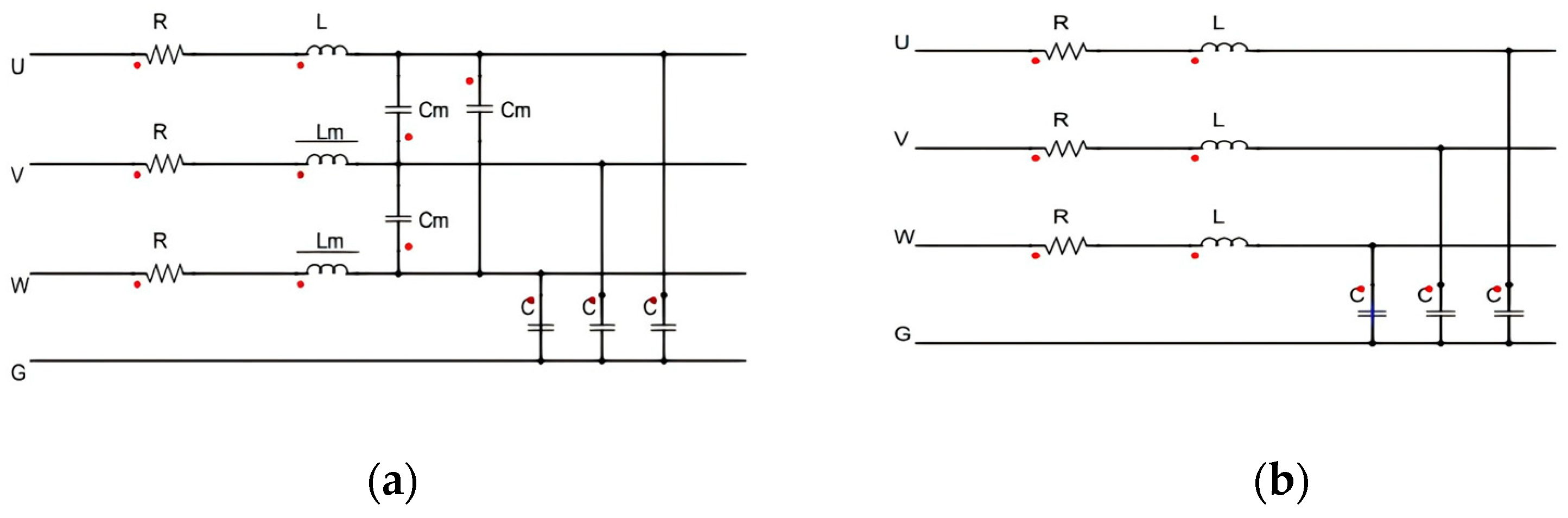
2.3. Motor Model

The high-frequency model of the motor is established by measuring the common-mode impedance $Z_{cm}$ and differential-mode impedance $Z_{dm}$ of the motor using an impedance analyzer. Numerical fitting methods are then employed to fit the amplitude characteristic curves of the motor’s port impedance, which allows for the calculation of the motor’s equivalent circuit model. Figure 6 shows the equivalent circuit model of the motor.

According to the circuit principles of the motor, it is necessary to obtain the single-phase common-mode impedance $Z_{cm}$ and the single-phase differential-mode impedance $Z_{dm}$ in order to derive the circuit model of the motor. Figure 7 shows the frequency response curves of the single-phase common-mode and differential-mode impedances. The $Z_{cm}$ curve shows a decreasing and then increasing trend. In the low-frequency band, $Z_{cm}$ decreases with increasing frequency and reaches a minimum at a certain frequency, after which it starts to rise again as the frequency is further increased. The $Z_{dm}$ curve shows a more complex fluctuating variation, especially in the low-frequency band, where the value of $Z_{dm}$ is more stable, and several distinct peaks of $Z_{dm}$ appear as the frequency is increased. According to the circuit principles of the motor, it is necessary to obtain the single-phase common-mode impedance $Z_{cm}$ and the single-phase differential-mode impedance $Z_{dm}$ in order to derive the circuit model of the motor.

When the RLC resonant unit is used to fit the impedance amplitude frequency characteristics, if the impedance amplitude frequency characteristics first appear as a trough, the RLC series parallel connection is used for fitting, as shown in Figure 7b. If the number of troughs is four groups, four groups of RLC series and parallel structures are used to fit the single-phase common-mode impedance. On the contrary, if the impedance amplitude frequency characteristic first appears, the RLC is connected in parallel and then connected in series, as shown in Figure 7a. If there are four groups of peaks, the four groups of RLC are fitted in parallel and then connected in series. In practical applications, in order to improve the fitting accuracy, two compensated RLC parallel circuits will be added to further fit the single-phase differential-mode impedance.

The impedance frequency response characteristics of the motor are obtained through RLC resonant element fitting, thereby establishing the equivalent circuit model of the motor. A series resonant circuit is used to establish the motor’s common-mode impedance circuit, while a parallel resonant circuit is employed for the motor’s differential-mode circuit. Ultimately, the motor’s equivalent circuit is established in Simplorer, as depicted in Figure 8.

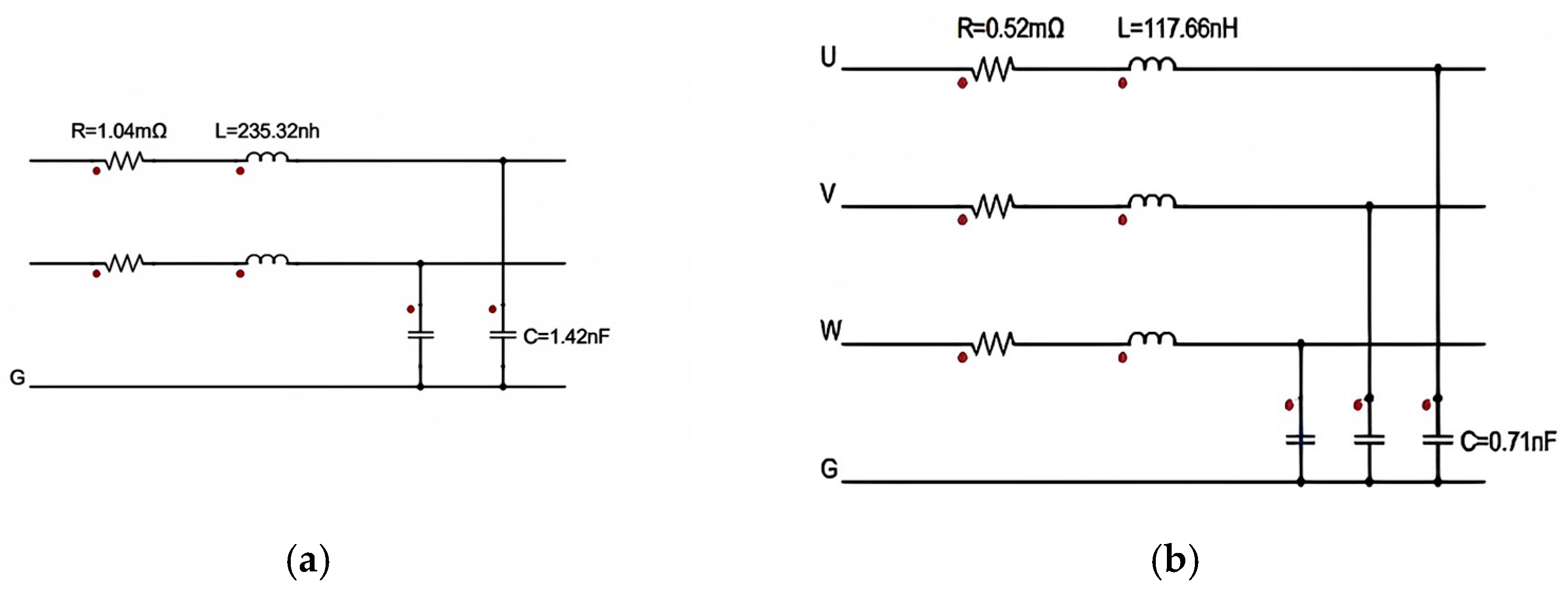
2.4. Cable Model

This paper adopts the theory of multi-conductor transmission lines to establish the cable model. Taking a three-phase AC busbar as an example, the diagram shows the multi-conductor transmission line model of the cable as illustrated. The diagram depicts the per unit length parameters of the transmission line, including the inductance per unit length, the resistance per unit length R, the parasitic capacitance C between conductors and shielding layers, the mutual inductance $L_m$ between transmission lines, and the mutual capacitance. In practical scenarios, the cables used typically include shielding layers; hence, the inter-phase mutual capacitance C can be considered negligible. Additionally, assuming that the spacing between cables of each phase is greater than 50 mm, the mutual inductance L between internal conductors is assumed to be 0. This results in a simplified multi-conductor transmission line model, as depicted in Figure 9.

This paper uses the theory of transmission lines to simulate polyethylene-insulated cables. According to the technical parameter guide manual, the cross-sectional structure is obtained, as shown in Figure 10.

According to the technical guide manual, dimensions r1, r2, r3, and r4 are, respectively, 5.75 mm, 4.75 mm, 4.35 mm, and 3.25 mm. Based on transmission line theory, the unit length parameters are calculated by a Maxwell 2D finite element simulation. Resistance R: skin effect leads to the increase in high-frequency resistance, R = 0.52 mΩ at 1 MHz. Inductance L: shielding layer reduces mutual inductance, L = 117.66 nH. Capacitance C: the capacitance between the shielding layer and the conductor C = 0.71 nF., as shown in

Table 2. Parameters of the simplified model.

Per Unit Length Resistance R	Capacitance C	Inductance L
0.52 mΩ	0.71 nF	117.66 nH

.

In practical situations, due to the longer distance from the battery to the inverter, the simulation model assumes a 2 m length for the DC busbar and a 1 m length for the AC busbar. Incorporating the above data yields the simplified models for the DC and AC busbars, as depicted in Figure 11.

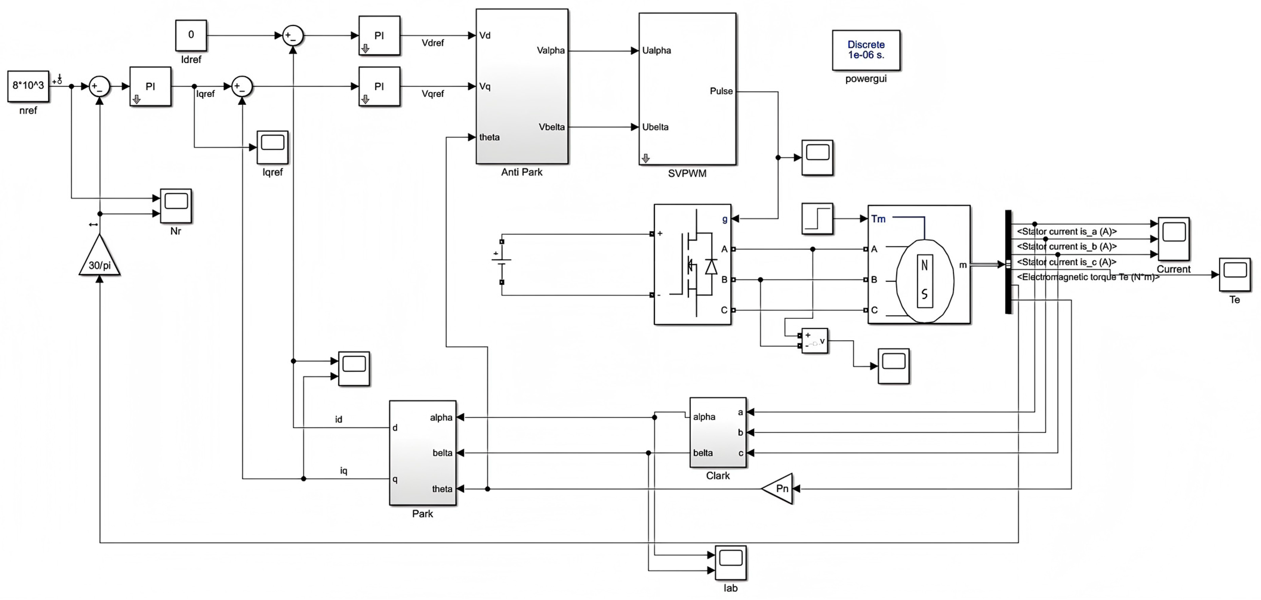
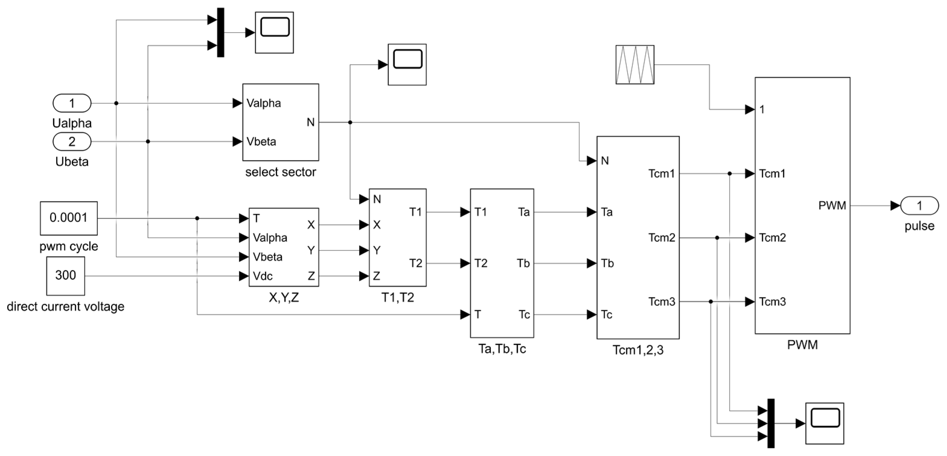
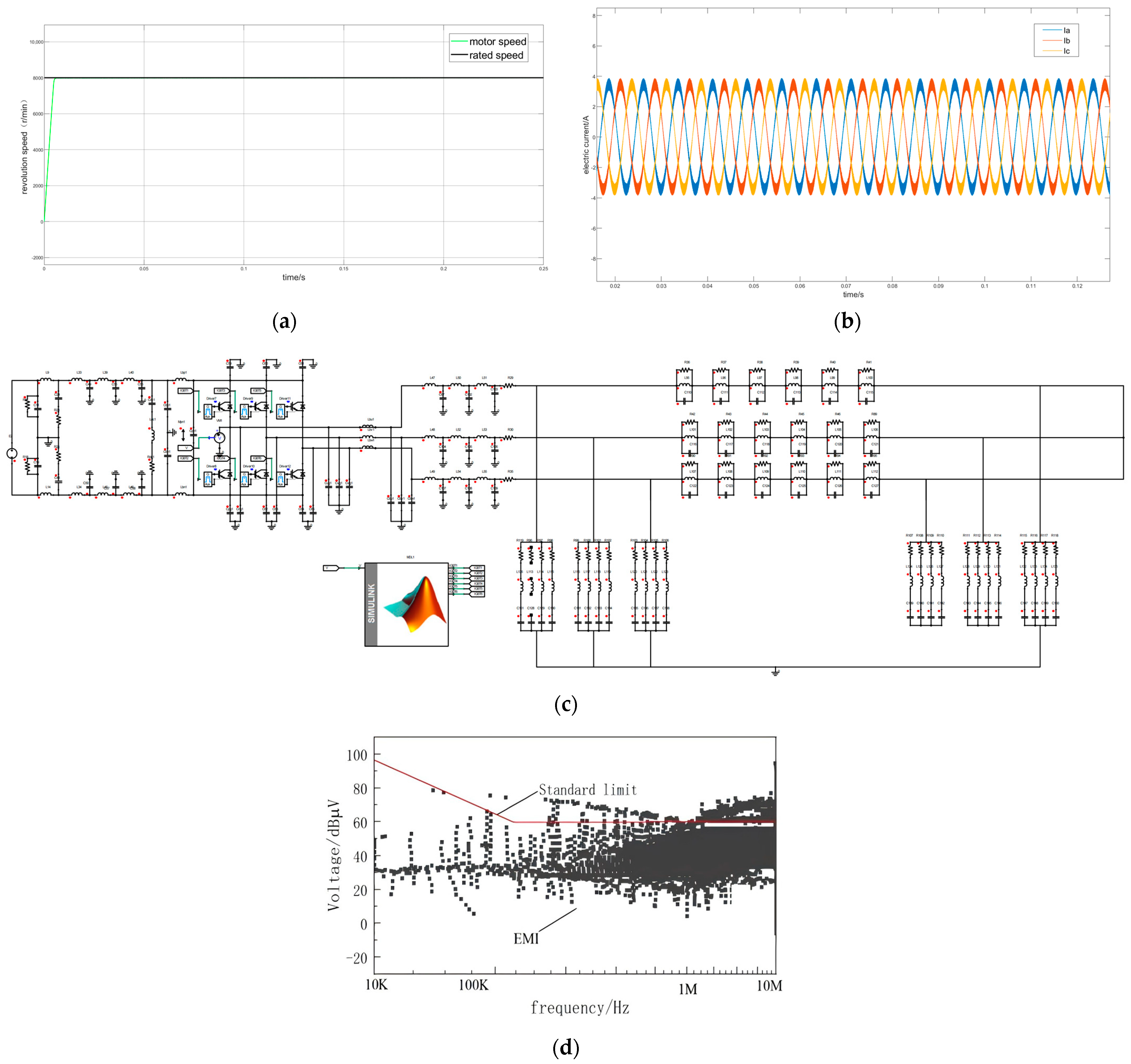
2.5. Control Model

Permanent magnet synchronous motors (PMSMs) have become a popular choice for electric vehicles due to their high efficiency, high power density, and fast response characteristics [21]. To achieve precise control of the motor and enhance its operational efficiency and performance, the control model used in this paper adopts a speed and current dual-loop control method and studies and analyzes it in MATLAB/Simulink 2021. The simulation model is shown in Figure 12.

It can be seen from Figure 12 that the whole system is a closed-loop control system based on negative feedback. After setting the initial speed, the system runs for a period of time. If the controller is effective, the actual output signal of the system will be fed back within a certain period of time, resulting in an error between the initial value and the set value and the input signal of the speed loop PID controller, that is, the speed error. Through the adjustment of the speed loop PID controller, the control quantity $i_q$ is adjusted so as to realize the accurate control of the motor speed. In the current loop, the three-phase current is converted into the d-q axis current component in the synchronous rotating coordinate system by current sampling and Clarke and Park transformation. The error between the q-axis current obtained by feedback and the $i_q$ output by the speed loop PID controller is used as the input signal of the q-axis current loop PID controller. At the same time, since the system runs in the (i_d = 0) mode, the error between the d-axis current and the zero value obtained by the feedback is also used as the input signal of the d-axis current loop PID controller. Under the action of the current loop PID controller, the d-q axis reference voltage in the synchronous rotating coordinate system is adjusted. The reference voltage in the two-phase stationary coordinate system is obtained by inverse Park transformation. The reference voltage is used as the input signal of the SVPWM module. After a series of processing steps, the reference voltage vector of the motor is finally obtained. At this time, the ideal trajectory of the voltage reference vector is circular, generating a circular magnetomotive force, thereby driving the motor rotor to achieve the adjustment of the speed of the permanent magnet synchronous motor.

In this paper, the speed–current double-loop control (Figure 9) is adopted, and its core improvements include the following:

SVPWM algorithm: Space vector pulse width modulation (SVPWM) significantly improves the utilization of DC bus voltage by optimizing the synthesis path of voltage vectors (the theoretical utilization rate can reach 100%, while the traditional sinusoidal PWM is only 86.6% [22]). In order to verify its harmonic suppression ability, the simulation comparison is carried out under the condition of rated current 450 A and switching frequency 10 kHz. The results show that the total harmonic distortion (THD) of SVPWM is 4.2%, while that of sinusoidal PWM is 7.8%. Compared with sinusoidal PWM, SVPWM can effectively reduce the harmonic distortion of the output voltage by selecting the optimal switching sequence. This low-harmonic characteristic is derived from the symmetrical distribution of space vectors by SVPWM, which reduces the current mutation during the switching process [23].

In addition, SVPWM significantly reduces high-frequency switching noise by suppressing high-frequency voltage spikes. Its core mechanisms include the following:

• Optimize the dead-time: by dynamically adjusting the dead-time compensation, the voltage overshoot during the switching of the switch tube is reduced [24].
• Vector smooth transition: Using a seven-stage or five-stage switching mode to avoid sharp jumps between adjacent vectors reduces electromagnetic interference (EMI) energy distribution [25]. The SVPWM model is established as shown in Figure 13.
• Current loop dynamic compensation: by adjusting the d-q axis current error in real time, the torque response time is shortened to 2 ms (the traditional model is 5 ms).
• Integrated EMI modeling: The conducted EMI sub-module is embedded in Simulink to monitor PWM harmonic distribution in real time.
• Dead-time optimization algorithm: an adaptive dead-time compensation strategy is used to reduce the overshoot voltage of the switch tube by 18%.

2.6. Co-Simulation

Based on the composition and operating principles of the motor drive system, the equivalent circuit models established above are interconnected in ANSYS/Simplorer, including the power supply, converter, and load sections. These circuit components include resistors, inductors, and capacitors, which together form a model of the system. Additionally, the motor control model is constructed in Simulink. Through the co-simulation of Simulink and Simplorer, a simulation predictive model for conducting EMI in the motor drive system is established, as shown in Figure 14c. The aim is to capture rapid changes in the system over a short period. The simulation is set with a duration of 0.25 s and a time step of $1\times {10}^8$ s. The simulation results, depicted in Figure 14, show the motor speed and current curves, as well as the predicted waveform of EMI.

From Figure 14, it can be observed that the frequency distribution of EMI exceeding the standard specified limits is above 100 kHz. The simulation indicates that the interference reaches a maximum of 87.05 dBμV at a frequency of 11 MHz. Based on these simulation results, comparison and analysis against standard limits yield an equivalent voltage source suitable for the quantitative design of EMI filters.

3. Filter Design

Filter design follows the following steps: differential and common-mode separation of EMI, determination of required insertion loss, selection of filter topology, and design of filter parameters [26].

3.1. Differential and Common-Mode Separation

Differential-mode interference is an interference signal that propagates in the opposite direction on two wires, which mainly affects power supply and signal integrity. The main sources are the switching noise of the inverter and the commutation process of the motor winding. Especially under the control of PWM (SVPWM), the switching frequency and harmonics will form strong differential mode interference. Through the DC bus, motor winding, drive circuit, etc., a closed loop propagation is formed.

Common-mode interference is an interference signal that propagates in the same direction on multiple conductors (usually between the phase line and the ground). It mainly affects the electromagnetic compatibility (EMC) of the system and is easy to radiate outward through cables, motor casings, and grounding circuits. The main sources are the transient change in the inverter switch, the parasitic capacitance of the IGBT module, the capacitance of the motor to the ground, and so on. It propagates through the motor shell, shielding layer, power line to the ground circuit, and other paths and may affect the external equipment through electromagnetic radiation.

Conducted EMI on power input lines can be represented by common-mode (CM) and differential-mode (DM) components, both of which can be independently suppressed in research. Differential- and common-mode waveforms obtained through co-simulation are shown in Figure 15.

Combining Figure 15 reveals the distribution pattern of conducted EMI. Below 500 kHz, differential-mode interference typically predominates. Between 500 kHz and 5 MHz, there is a mixture of both differential-mode and common-mode interference. Above 5 MHz, common-mode interference becomes predominant.

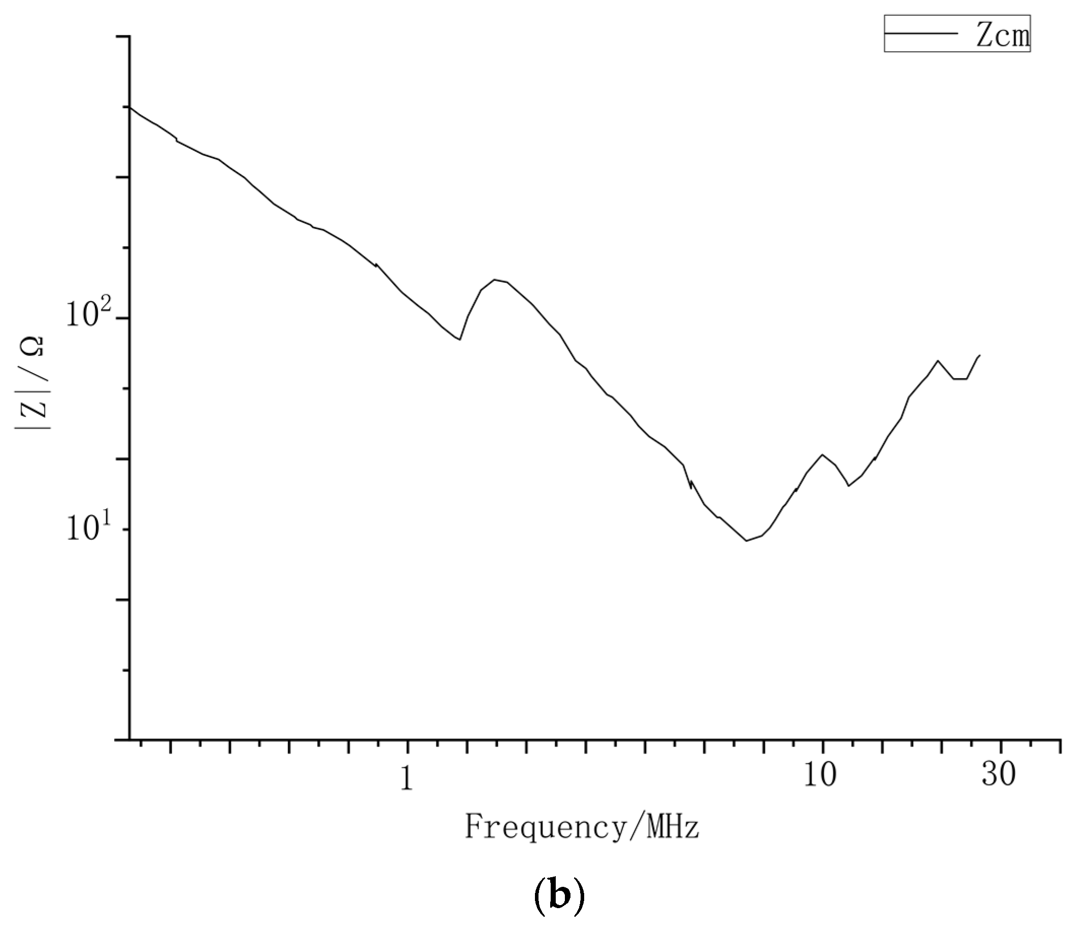
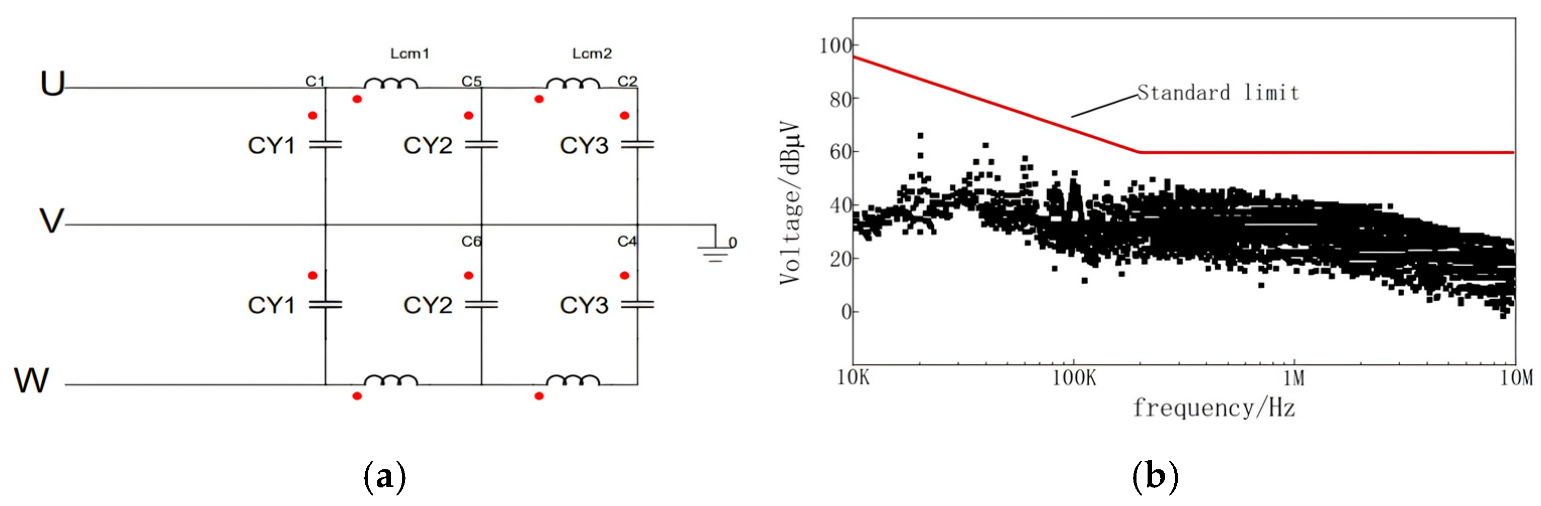
3.2. Common-Mode Filter Design

Common-mode interference is the sum of currents flowing from the phase and neutral points to the ground. This noise is typically generated by switching-induced pulses or the capacitive effects of filtering capacitors and MOSFET heatsinks. With the aid of the co-simulation model, the voltage and current of common-mode interference are obtained as follows:

$$V_{cm}={\displaystyle \frac{V_p+V_n}{2}}$$

(1)

$$I_{cm}=I_p+I_n$$

(2)

where $V_{cm}$ is the common-mode voltage, $V_{cm}$ is the phase voltage, $V_n$ is the neutral voltage, $I_{cm}$ is the common-mode current, $I_p$ is the phase current, $I_n$ is the neutral current, $V_p$ is the phase voltage, and $V_n$ is the neutral voltage.

To ensure high-frequency EMC performance, the same cutoff frequency is set for single-stage L-type and Π-type filters for circuit simulation. The results, as shown in Figure 16, indicate that the L-type filter has a slope of 40 dB/decade, but due to parasitic parameter effects, insertion loss deteriorates in the high-frequency range and may even fail. The Π-type filter exhibits a slope of 60 dB/decade up to 2 MHz and 100 dB/decade from 2 MHz to 30 MHz. Considering overall performance, the Π-type filter outperforms the L-type filter across the frequency range of 150 kHz to 30 MHz.

Although the simulation results show that the Π-type filter is superior to the L-type filter in terms of EMI suppression in practical applications, in addition to considering performance, factors such as design difficulty, cost, volume, and durability need to be weighed. The Π-type filter has high design complexity and difficulty in implementation. It requires multiple precise inductors and capacitors, high cost, and large volume, which may pose challenges in space-constrained applications. However, its superior high-frequency noise suppression ability makes it perform well in occasions with high requirements for EMI suppression. In contrast, the L-shaped filter is simple in design, low in cost, small in size, and strong in durability. It is suitable for low-frequency or medium-frequency interference suppression, and the difficulty of implementation is low. It is suitable for environments with limited budget and compact space. Nevertheless, from the perspective of overall performance and high-frequency interference suppression requirements, the application of Π-type filters in electric vehicle motor drive systems is still a better choice.

Based on the simulated results of common-mode interference, considering the use of a second-order Π-type filter, the filter circuit is incorporated as shown in Figure 14. The cutoff frequency calculation is as follows:

$$V_a=V_e+6\mathrm{d}\mathrm{B}$$

(3)

$$f_{CM}={\displaystyle \frac{1}{2\pi \sqrt{\left(L_{CM}+\frac{L_{DM}}{2}\right)·2C_Y}}}$$

(4)

where $f_{CM}$ is the common-mode cutoff frequency, $V_a$ is the attenuation voltage, $V_e$ is the excess voltage, 6 dB is the safety margin, $L_{CM}$ is the common-mode inductance, and $C_X$ and $C_Y$ are differential- and common-mode capacitors, respectively.

Combining Equations (1) and (4) with the suppression requirements, filter parameters can be determined through calculation and simulation. The final parameters are shown in

Table 3. Final parameters for common mode filter design.

${\mathit{C}}_{\mathit{Y}1}$	${\mathit{C}}_{\mathit{Y}2}$	${\mathit{C}}_{\mathit{Y}3}$	${\mathit{L}}_{\mathit{C}\mathit{M}}$
1 nF	0.3 nF	0.5 nF	6 mH

. In the co-simulation model, a second-order Π-type common-mode filter is integrated, and the test results are shown in Figure 17. It can be observed that after integrating the common-mode filter, especially in the high-frequency range of 150 kHz to 30 MHz, the system’s common-mode interference is below the conducted interference standard limits.

3.3. Differential-Mode Filter Design

Differential-mode interference is the current generated by the difference in phase voltage and neutral voltage. It arises from interactions between circuit components. Using a combined simulation model, the voltage and current of differential-mode interference are obtained as follows:

$$V_{dm}=V_p+V_n$$

(5)

$$I_{dm}={\displaystyle \frac{I_p-I_n}{2}}$$

(6)

where $V_{dm}$ is the differential-mode voltage and $I_{dm}$ is the differential-mode current. Based on the insertion loss comparison between L-type and Π-type filters from Figure 13 and considering the simulated results of differential-mode interference, a first-order Π-type filter is considered. The filter circuit is integrated as shown in Figure 15. The cutoff frequency calculation is as follows:

$$V_a=V_e+6\mathrm{dB}$$

(7)

$$f_{DM}={\displaystyle \frac{1}{2\pi \sqrt{2L_{DM}\times \left(C_X+\frac{C_Y}{2}\right)}}}$$

(8)

where $f_{DM}$ is the differential-mode cutoff frequency and $L_{CM}$ is the differential-mode inductance. Combining Equations (5) and (8) with the suppression requirements, filter parameters are determined through calculation and simulation. Adjusting the filter to a balanced configuration to assist in common-mode suppression, the final parameters are shown in

Table 4. Final parameters for differential mode filter design.

${\mathit{C}}_{\mathit{X}1}$	${\mathit{C}}_{\mathit{X}2}$	${\mathit{L}}_{\mathit{D}\mathit{M}}$
3.5 µF	3 µF	5.8 µH

.

In the co-simulation model, a Π-type differential-mode filter is integrated, and the test results are shown in Figure 18. It can be observed that after integrating the differential-mode filter, differential-mode interference across the frequency range of 150 kHz to 30 MHz is below the conducted interference standard limits.

4. Experimental Validation

The designed filter is simulated and analyzed by a Matlab–Simplorer co-simulation platform. In addition to the above common-mode sum difference simulation of the filter, Figure 19 shows the filter’s electromagnetic interference suppression results for the full frequency band. The interference voltage spectrum diagram after adding the filter is compared with the voltage spectrum diagram in the second chapter. It can be seen that before adding the filter, the maximum peak value of the interference voltage of the motor drive system is 87.05 dBμV. After adding the filter, the maximum peak value in the range of 11 Mhz is reduced, which is reduced by about 40 dBμV. The suppression effect of the filter on the conducted electromagnetic interference of the motor drive system is further proved.

5. Conclusions

Aiming at the electromagnetic interference (EMI) problem of electric vehicle motor drive systems, this study constructs a joint simulation model of the coupling characteristics of each device and quantitatively analyzes the mechanism of differential-mode and common-mode interference. The optimized motor control model adopts a double closed-loop control of speed and current, which improves the dynamic response and stability of the system and enhances the matching degree of the simulation results to the actual operation and EMI characteristics of the motor. The simulation model provides a reliable theoretical basis for electromagnetic compatibility (EMC) design and helps to improve the EMC performance of the system.

In addition, the simulation model is used to quantitatively design the filter, which realizes the independent optimization of differential-mode and common-mode interference, avoids redundant design, and improves the accuracy of filter parameter selection. Based on the simulation results, the filter order and parameters are reasonably adjusted, which not only improves the EMI suppression effect but also reduces the design complexity and cost.

References

- Shuo, Z.; Xuerong, L.; Xing, C.; Yang, W.; Chengning, Z. Parameter disturbance suppression method of PMSM. Trans. Beijing Inst. Technol. 2022, 42, 184–191. (In Chinese) [Google Scholar]
- Jiang, X. A Brief Analysis of the Differences and Connections between Electromagnetic Interference in Pure Electric Vehicles and Fuel Vehicles. Automot. Electr. Appl. 2018, 8, 11–12. [Google Scholar]
- Xu, X.; Chen, W.; Liu, C.; Chen, N.; Wang, F.; Wang, Y.; Zhang, K.; Ma, Y.; Zhang, S.; Zhou, Q.; et al. A Novel IGBT with Self-Regulated Potential for Extreme Low EMI Noise. IEEE Electron Device Lett. 2018, 40, 71–74. [Google Scholar] [CrossRef]
- Sun, R.; Deng, X.; Li, X.; Li, X.; Wu, H.; Wen, Y.; Zhang, B. A Novel SiC Trench MOSFET Embedding Auto-Adjust Source-Potential Region with Switching Oscillation Suppression. IEEE Electron Device Lett. 2023, 40, 1817–1820. [Google Scholar] [CrossRef]
- Fan, G. A brief discussion on the generation mechanism of electromagnetic interference in the motor drive of new energy vehicles. Times Automob. 2023, 112–114. [Google Scholar]
- Li, H.; Tang, S.; Wang, J. Electromagnetic compatibility design of in-cabin fan for space station. Micro Spec. Mot. 2024, 52, 22–25. [Google Scholar]
- Alamsyah, M.S.; Vieira, F.L.; Garbe, H.; Koj, S. The Effect of Stray Capacitance to the Common Mode Current on Three-Phase System. In Proceedings of the 2021 IEEE International Joint EMC/SI/PI and EMC Europe Symposium, Raleigh, NC, USA, 26 July–13 August 2021; pp. 430–433. [Google Scholar]
- Middelstaedt, L.; Wang, J.; Stark, B.H.; Lindemann, A. Direct Approach of Simultaneously Eliminating EMI-Critical Oscillations and Decreasing Switching Losses for Wide Bandgap Power Semiconductors. IEEE Trans. Power Electron. 2019, 34, 10376–10380. [Google Scholar] [CrossRef]
- GB/T 33012.1-2016; Road Vehicles—Electromagnetic Compatibility of Vehicles—Part 1: Terminology and Definitions. China Standard Press: Beijing, China, 2016.
- Li, X.; Wang, L.; He, J. Research of the electromagnetic compatibility design technology of battery management system on electric vehicle. Int. J. Electr. Hybrid Veh. 2013, 5, 69–78. [Google Scholar] [CrossRef]
- Wang, Y.; Zheng, S.; Kang, X. Conducted electromagnetic interference modeling method for booster circuit of electronic safety system. J. Detect. Control 2024, 46, 63–69. [Google Scholar]
- Guo, Y.; Wang, L.; Liao, C. Systematic Analysis of Conducted Electromagnetic Interferences for the Electric Drive System in Electric Vehicles. Prog. Electromagn. Res. 2013, 134, 359–378. [Google Scholar] [CrossRef]
- Yang, Y.M.; Peng, H.M.; Wang, Q.D. Common Model EMI Prediction in Motor Drive System for Electric Vehicle Application. J. Electr. Eng. Technol. 2015, 10, 205–215. [Google Scholar] [CrossRef]
- Duan, Z.; Wen, X. A new analytical conducted EMI prediction method for SiC motor drive systems. eTransportation 2020, 3, 100047. [Google Scholar] [CrossRef]
- Yang, M.; Lyu, Z.; Xu, D.; Long, J.; Shang, S.; Wang, P.; Xu, D. Resonance Suppression and EMI Reduction of GaN-Based Motor Drive with Sine Wave Filter. IEEE Trans. Ind. Appl. 2020, 56, 2741–2751. [Google Scholar] [CrossRef]
- Li, Z.; Shuangjie, Y.; Guixing, H.; Shuliang, W. Modeling of Conducted Electromagnetic Interference in Electric Vehicle Motor Drive System. J. Beijing Inst. Technol. 2022, 42, 824–833. [Google Scholar]
- Kim, H.; Fan, J.; Lee, S.; Hong, S.; Sim, B.; Kim, J. Analytical Expressions of Differential-mode Harmonics in Loosely-coupled Series-resonant Wireless Power Transfer System. In Proceedings of the 2019 IEEE International Symposium on Electromagnetic Compatibility, Signal & Power Integrity (EMC+SIPI), New Orleans, LA, USA, 22–26 July 2019; 2019; pp. 648–653. [Google Scholar]
- Zhuo, Y.; Donghai, L.; Liu, Y.; Rongxun, J.; Wei, S. Research on EMC simulation technology of electric vehicle drive system based on ANSYS. China Automot. 2020, 9, 53–57. [Google Scholar]
- Chen, P.; Chen, W.; Li, B. EMI model of permanent magnet synchronous motor based on vector fitting method. J. Power Supply 2021, 19, 126–133. [Google Scholar]
- Kumar, S.M.; Rani, J.A. Reduction of conductedelectromagnetic interference by using filters. Comput. Electr. Eng. 2018, 72, 169–178. [Google Scholar] [CrossRef]
- Li, W.; He, Y. Parameterization and Performance of Permanent Magnet Synchronous Motor for Vehicle Based on Motor-CAD and OptiSLang. Wirel. Commun. Mob. Comput. 2022, 2022, 8217386. [Google Scholar] [CrossRef]
- Holtz, J. Pulsewidth Modulation for Electronic Power Conversion. IEEE Trans. Ind. Electron. 1992, 39, 410–420. [Google Scholar] [CrossRef]
- Bose, B.K. Power Electronics and Motor Drives: Advances and Trends; Academic Press: Cambridge, MA, USA, 2006. [Google Scholar]
- Li, R.; Xu, D. Dead-Time Compensation for SVPWM-Based Motor Drives. IEEE Trans. Power Electron. 2015, 30, 3457–3465. [Google Scholar]
- Zhang, Y. EMI Reduction in SiC Motor Drives via Optimized SVPWM. IEEE Trans. Electromagn. Compat. 2020, 62, 812–820. [Google Scholar]
- Xu, H.; Luo, S.; Bi, C.; Sun, W.; Zhao, H.; Liu, J. Design of broadband hybrid EMI filter based on SiCMOSFET synchronous BuckDC-DC converter. Trans. China Electrotech. Soc. 2024, 39, 3060. [Google Scholar]