Lamb Wave Near-Field Source Localization Method for Corrosion Monitoring

Abstract

Corrosion is one of the main causes of aircraft structural damage. The deepening of the corrosion depth will greatly endanger the safety of the crew. The Lamb wave array signal processing method can be used to estimate the direction of arrival (DOA) of the signal source. As a form of the Lamb wave array signal processing method, multiple-signal classification (MUSIC) has been gradually applied to the corrosion monitoring of aluminum plates. However, when MUSIC is used for Lamb wave DOA estimation, it has a low resolution and poor anti-interference ability. To improve it, the Lamb wave near-field source location (LWNFL) method is proposed in this paper. The new method adopts a double-sensor array arrangement. Firstly, the compressed sensing (CS) theory is combined with the Lamb wave near-field array model to obtain a DOA estimation of the corrosion. Here, the corrosion angle can be obtained using a CS reconstruction algorithm, and the noise interference can be suppressed by limiting a minimization of the l₂ norm. Then, the corrosion distance is calculated according to the Lamb wave arrival time difference between different sensors. Finally, the average of the positioning results from multiple excitation sensors is used as the final location of the corrosion. The proposed LWNFL method is verified on an aluminum plate. The experimental results show that the new method can accurately obtain the location of corrosion and has good resolution and strong anti-interference ability.

1. Introduction

Corrosion is one of the main reasons for surface damage to aircraft structures, and it is a kind of damage that occurs gradually and deepens with the continuation of the working time [1]. For aircraft, especially aging aircraft, due to the influence of the flight environment, corrosion damage accompanying the service process is ubiquitous. Once an aircraft structure is corroded, the shape and strength of the structure will be seriously affected [2]. When the corrosion damage reaches a certain level, it may cause serious flight accidents and greatly endanger the safety of the crew.

Early corrosion damage to aircraft structures has the characteristics of a small area and easy concealment. Structural health monitoring (SHM) based on Lamb waves has the advantages of being sensitive to small damages and able to realize regional monitoring. It is more suitable for aircraft than traditional methods such as visual inspection and non-destructive testing. SHM based on Lamb waves uses piezoelectric (referred to as PZT) sensors arranged on the structure to excite Lamb waves, and then the Lamb wave response signals are received by other PZT sensors fixed to the structure. By analyzing the reference signals in the no-damage state and the monitoring signals after damage occurs, the characteristic parameters can be extracted, especially when the PZT sensor array is arranged, the online monitoring of the damage in a certain range of aircraft structures can be realized [3,4,5]. Therefore, in recent years, more and more researchers have used it for the corrosion monitoring of structures [6,7,8,9,10].

The principle of array signal processing is to arrange multiple sensors in a space into an array, receive and process spatial signals, obtain the required characteristic information, and suppress noise or disinteresting information interference [11]. As a classical algorithm in array signal processing, the multiple signal classification (MUSIC) algorithm divides the data received by the sensor array into signal subspaces and noise subspaces, then uses the orthogonality of signal subspace and noise subspace to search the spatial spectrum of the space to be monitored so as to realize the DOA estimation of the signal source. The MUSIC algorithm adopts dense sensor array layouts, which are easily deployed on complex aviation structures and can realize directional scanning on structures with a large monitoring range. At present, the MUSIC algorithm and its derivatives have been applied in the field of SHM based on Lamb waves.

Engholm M et al. [12] used the MUSIC algorithm to estimate the direction of an excitation source in a uniform circular array. Yang H et al. [13] adopted the MUSIC algorithm to realize the impact location on the metal aluminum plate and calculated the distance from the impact source to the reference element by using the geometric relationship between the impact source and the sensor array. Since most impacts on aircraft structures occur near the array, Yuan S F et al. [14,15,16] proposed a near-field 2D-MUSIC impact positioning method, which simultaneously realized the location of the impact source angle and distance by establishing a near-field signal model. The impact positioning experiment was verified on the anisotropic composite plate. Subsequently, Zhong Y T et al. [17] applied the near-field 2D-MUSIC method to the damage location and conducted experimental verification on the structure of the carbon fiber composite plate and aviation composite fuel tank. Bao Q et al. [6] proposed a MUSIC corrosion damage location method based on excitation beam formation, which increased the amplitude of the excitation signal via superposition of multiple excitation signals and enhanced the anti-interference performance of the method. This method was used to monitor the position of the corrosion of an aluminum plate.

The MUSIC algorithm based on Lamb waves can be used to locate damage to a structure. However, when the MUSIC algorithm is used for DOA estimation, it is sensitive to noise and has poor anti-interference ability, which requires a high signal-to-noise ratio of the received signal and the number of signal sources to be known in advance. These shortcomings limit the application of the MUSIC algorithm in corrosion damage monitoring of aircraft structures.

The improved DOA estimation algorithms mainly include the variable step size least mean square (VSS-LMS) algorithm [18], the error censoring-based recursive least square (EC-RLS) algorithm [19], the root-MUSIC algorithm [20], the maximum likelihood (ML) DOA estimation algorithm [21,22], the deep learning (DL) DOA estimation algorithm [23,24], and the CS-based DOA estimation algorithm. These algorithms improve the deficiency of the MUSIC algorithm in DOA estimation, among which the VSS-LMS algorithm and the EC-RLS DOA algorithm simplify the computational complexity. The root-MUSIC algorithm, the ML DOA estimation algorithm, the DL DOA estimation algorithm, and the CS-based DOA estimation algorithm have a better resolution than the MUSIC algorithm.

However, for DOA estimation based on Lamb waves, only a set of Lamb wave signals needs to be excited when conducting structural damage monitoring. The sensor array receives this set of data and processes it. Generally, this set of signals is 5000–10,000 points. Therefore, in the field of Lamb wave-based SHM, the computational complexity of the MUSIC algorithm is low, and the VSS-LMS algorithm and the EC-RLS DOA algorithm have no advantage.

In addition, the resolution improvement effect of the R-MUSIC is not obvious. ML DOA estimation algorithm requires a multi-dimensional search, which increases the complexity of the algorithm. The DL DOA estimation algorithm needs to receive multiple sets of data for training to accurately locate the DOA of the signal source. Therefore, these algorithms are not suitable for DOA estimation based on Lamb waves.

Compressed sensing (CS) theory was proposed by Donoho D L, Candes E J, and Tao T in 2006 [25,26,27]. Now, CS has become a well-understood fundamental theory within the industry. By solving an underdetermined equation, CS can obtain the original high-dimensional sparse signal from a small number of acquired signals. It can suppress the noise using mathematical methods and provides a new idea for direction of arrival (DOA) estimation. Therefore, researchers have combined CS with DOA estimation in recent years. Using CS modeling, the space containing signal sources can be discretized and under-sampled into the array receiving signals. Then, the space angles where signal sources are located are estimated from a small number of signals received by the sensor array using the CS reconstruction algorithm. DOA estimation based on CS obtains angles of signal sources by calculating the minimum of the l₁ norm. It can suppress the noise by restricting the minimization of the l₂ norm. With a mathematical calculation, it can improve the anti-interference ability. Due to this advantage, CS has opened a new method for DOA estimation and has broad application prospects. Malioutov D M et al. [28] introduced CS into DOA estimation. Since then, the CS theory has been used in the DOA estimation of array signals [29,30,31,32,33,34].

Although the DOA estimation based on CS has many advantages and has been widely used at present, there are few research studies and applications in the field of SHM based on Lamb waves, especially in the monitoring of corrosion damage, and further research studies are needed. In order to improve the shortcomings of the MUISC in DOA estimation and achieve an accurate location of the corrosion angle in the structure, this article proposes Lamb wave near-field source localization (LWNFL). The new method adopts a dual-array sensor arrangement that consists of an excitation source array and a sensor array. Firstly, the new method estimates the corrosion angle using the Lamb wave near-field DOA estimation based on CS, which estimates the angle of corrosion by solving an optimization equation. Then, the distance of corrosion is calculated by the propagation speed of the Lamb wave in the aluminum plate and the time difference of receiving the Lamb wave using different sensors in the array. In addition, in order to increase the accuracy of corrosion location, the new method uses the average value of positions obtained by multiple excitation sensors as the final corrosion location. The verification experiment is carried out in an aluminum plate with artificial corrosion, and the results prove the superiority of the proposed method.

In Section 2, Lamb wave near-field DOA estimation based on CS is studied. In Section 3, Lamb wave near-field distance estimation is introduced. In Section 4, according to the angle estimation and distance estimation of near-field source, the LWNFL is proposed. In Section 5, experimental validation is carried out, and the performance of the new method and the MUSIC algorithm are compared. Finally, Section 6 provides the Discussion.

2. Lamb Wave Near-Field DOA Estimation Based on CS

2.1. Theory of CS

CS theory states that when the signal is sparse or sparse in a transform domain, the original sparse high-dimensional signal can be “under-sampled” into a low-dimensional signal by using a measurement matrix. Then, by solving the underdetermined equations, the original high-dimensional signal can be reconstructed accurately with high probability from the low-dimensional signal.

Assuming an n-dimensional real signal X ($X\in R^N$), it can be expanded into the following form under the orthonormal basis Ψ of the N × N dimension:

$$\mathit{X}=\mathbf{\Psi }\mathit{\alpha }$$

(1)

where a is an N-dimensional vector. K is the number of non-zero values in a. If K satisfies K << N, a is said to be K-sparse, then X is a compressible signal. Then, we can construct another M × N dimension (M < N) measurement matrix Φ unrelated to Ψ and perform an ‘under-sample’ on the N dimension (high-dimension) signal X to obtain M dimension (low-dimension) signal y. The under-sample process is as follows:

$${\mathit{y}}_{\mathit{M}\times 1}={\mathbf{\Phi }}_{\mathit{M}\times \mathit{N}}{\mathit{X}}_{\mathit{N}\times 1}={\mathbf{\Phi }}_{\mathit{M}\times \mathit{N}}{\mathbf{\Psi }}_{\mathit{N}\times \mathit{N}}{\mathit{\alpha }}_{\mathit{N}\times 1}={\mathbf{\Theta }}_{\mathit{M}\times \mathit{N}}{\mathit{\alpha }}_{\mathit{N}\times 1}$$

(2)

where a is a sparse vector, and Θ is the observation matrix. The observation matrix Θ is a bridge connecting the original sparse signal a and the measured signal y. In order to ensure that the received signal can maintain the original information after under-sampling, Baraniuk R G, ref. [35] proposed that the column vectors in the observation matrix Θ should be independent of each other.

For the equations formed by Equation (2), y is the measured M-dimensional signal, and the number of equations M is less than the dimension N of unknown vector a. Therefore, the equations have numerous groups of solutions. CS theory points out that as long as a is a sparse vector, the sparsest a obtained under the constraint condition $\mathit{y}=\mathrm{\Theta }\mathit{\alpha }$ is the required solution [18]. Its mathematical expression is as follows:

$${\mathbf{min}}_{\alpha }{‖\mathit{\alpha }‖}_0\hspace{1em}s.t.\hspace{1em}y=\mathrm{\Theta }\alpha$$

(3)

Here, we need find the minimum value of ${‖a‖}_0$. This optimization solution is an NP-hard non-convex problem with high computational difficulty. In order to avoid dealing with such complex problems directly, Tasig Y & Donoho D L [36] proved that the l₁ norm is equivalent to the l₀ norm when the columns of the observation matrix are irrelevant. That is, Equations (4) and (3) have the same solution.

$${\mathbf{min}}_{\mathit{\alpha }}{‖\mathbf{\alpha }‖}_1\hspace{1em}\mathit{s}.\mathit{t}.\hspace{1em}\mathit{y}=\mathbf{\Theta }\mathit{\alpha }$$

(4)

The solution of Equation (4) can be easily obtained by solving the linear programming problem. However, in practice, the measured signal y often contains noise signals, which is not considered in Equation (4). We suppose the measured signal y with noise is shown as Equation (5).

$$\mathit{y}=\mathit{\Theta }\mathit{\alpha }+\mathit{e}$$

(5)

where e is the noise vector. Equation (5) can also be expressed by the follow convex optimization problem with constraints [36].

$$\mathbf{min}{‖\mathit{y}-\mathbf{\Theta }\mathit{\alpha }‖}_2+\lambda {\left|\right|\mathit{\alpha }\left|\right|}_1$$

(6)

where λ is a sparse parameter, and its value is determined according to the noise intensity. For Equation (6), there is already a relatively mature solution method, and the sparse vector a can be easily solved by using the convex optimization toolbox cvx in matlab (version number: v9.9.0.1467703).

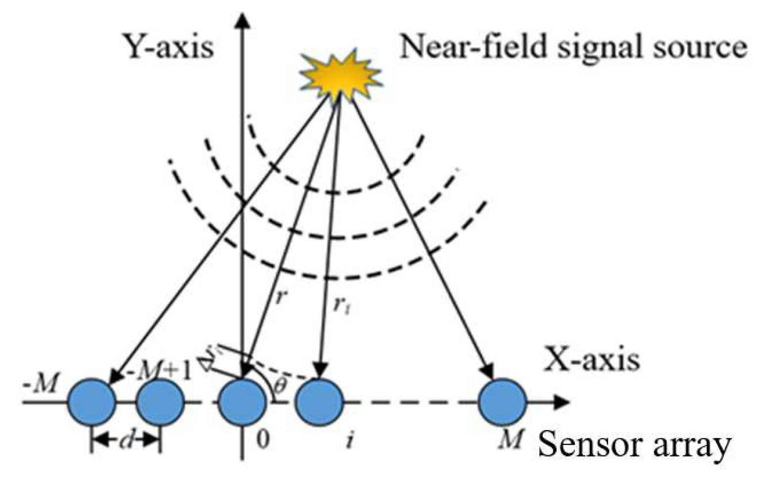
2.2. Lamb Wave Near-Field Array Model

The objective of this paper is to realize the location of corrosion on the aircraft structure, and the monitoring object is the corrosion in a narrow area of the aircraft structure. Therefore, the Lamb wave near-field model is used in this paper. Suppose there is a one-dimensional uniform linear PZT sensor array receiving a Lamb wave signal; the array element number is 2M + 1, and the array spacing is d. When the signal source is close to the sensor array, the response signals received by the array are a spherical wave. The signal propagation model of the Lamb wave array is shown in Figure 1, where the reference element is PZT 0, and the polar coordinate of the signal source is assumed to be (r, θ)—that is, r is the distance between the signal source and the reference element, and $\theta$ is the angle of the signal source relative to the reference element.

The received signal of the reference element PZT0 in the array can be written as

$$x_0\left(t\right)=u\left(t\right)e^{j\left({\omega }_{0}t-kr\right)}$$

(7)

where u(t) is the amplitude of the signal source. k = ω₀/c is the Lamb wave number, ω₀ is the center frequency of Lamb wave signal, and c is the propagation velocity of Lamb wave. The received signal of each array element is related to the distance from the signal source to it. Therefore, according to the distance relationship between other array element PZTi and reference array PZT0, received signal of array element PZTi can be represented by the received signal of the reference array element and the distance difference between them; its expression is shown in Equation (8):

$$x_i\left(t\right)=u\left(t\right)e^{j\left({\omega }_{0}t-k\left(r+\Delta r_i\right)\right)}=u\left(t\right)e^{j\left({\omega }_{0}t-kr\right)}{e}^{-j{\omega }_0\left(\Delta r_i/c\right)}=x_0(t)e^{-j{\omega }_0\left(\Delta r_i/c\right)}$$

(8)

where Δr_i is the distance difference for the signal source to PZTi relative to the signal source to PZT0. The Lamb wave time delay difference τ_i between signal source propagation to PZTi and signal source propagation to PZT0 can be expressed as Equation (9):

$${\tau }_i={\displaystyle \frac{\Delta r_i}{c}}={\displaystyle \frac{r-r_i}{c}}$$

(9)

Therefore, the received signal of the sensor array can be represented by the received signal of the reference array and the exponential function of time delay τ_i:

$$x_i\left(t\right)=x_0(t)e^{-j{\omega }_0{\tau }_i}$$

(10)

The path from the signal source to PZT0 and PZTi and the connecting lines of PZT0 and PZTi can form a triangle. Therefore, the distance r_i propagated by the signal source to each element of the sensor array can be expressed as

$$r_i=\sqrt{r^2+i^2\cdot d^2-2r\cdot i\cdot d\cdot \cos \theta },i=-M,-M+1,\dots ,M$$

(11)

where i refers to the serial number of sensor. By substituting Equation (11) into Equation (9), the expression of time delay in the near-field case can be written as

$${\tau }_i={\displaystyle \frac{r-\sqrt{r^2+i^2\cdot d^2-2r\cdot i\cdot d\cdot \cos \theta }}{c}},i=-M,-M+1,\dots ,M$$

(12)

We can define the vector a_i(r,θ) in the near-field as

$$a_i\left(r,\theta \right)=e^{-j{\omega }_0{\tau }_i}$$

(13)

Therefore, in the case of Lamb wave near-field array, signals received by the sensor array can be written as

$$\left[\begin{array}{c}{x}_{-M}\left(t\right)\\ x_{-M+1}\left(t\right)\\ ⋮\\ x_M\left(t\right)\end{array}\right]=\left[\begin{array}{c}{a}_{-M}\left(r,\theta \right)\\ a_{-M+1}\left(r,\theta \right)\\ ⋮\\ a_M\left(r,\theta \right)\end{array}\right]x_0\left(t\right)$$

(14)

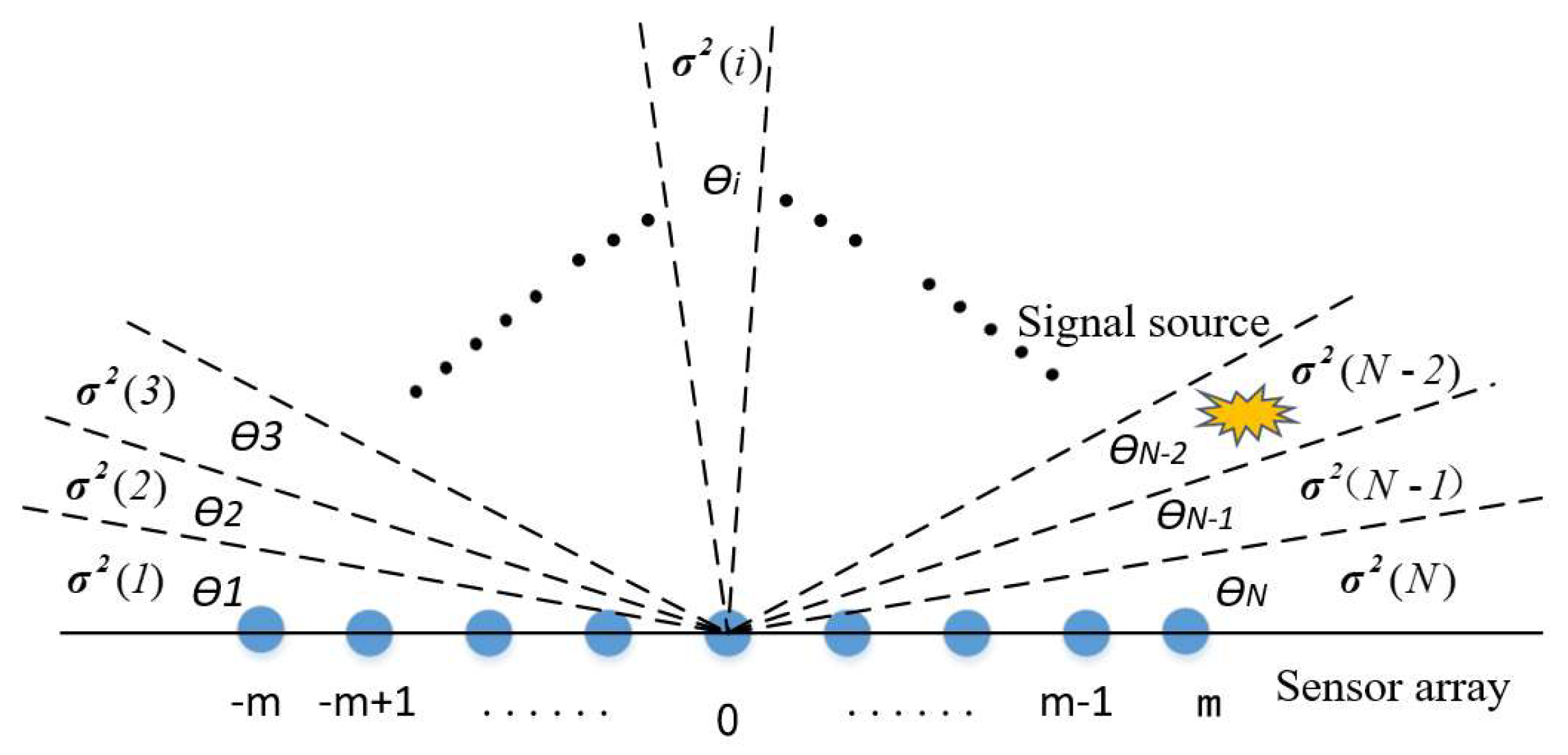
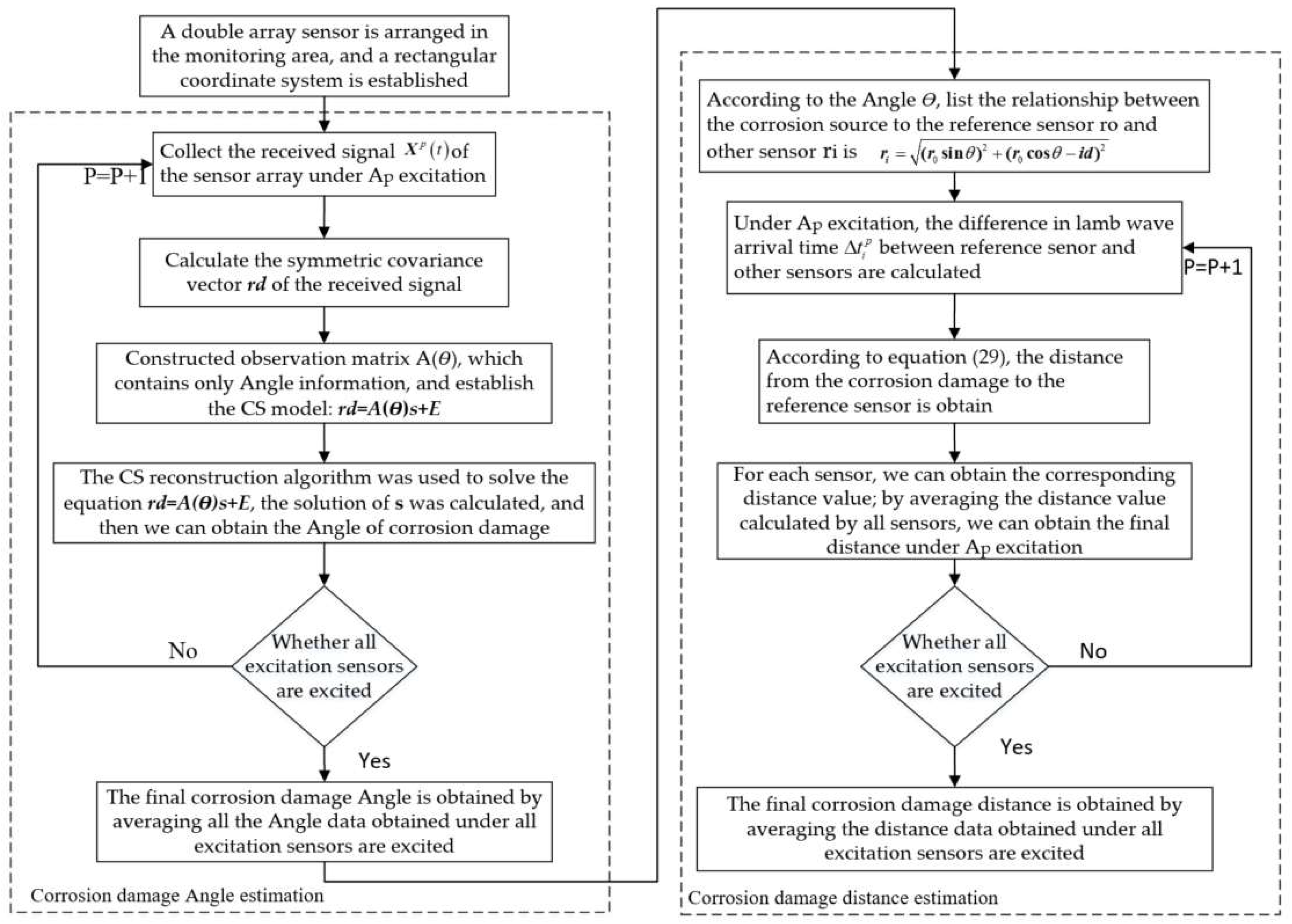
2.3. DOA Estimation Based on CS

If the CS model is established according to Equation (14), we need to divide the space into grids by the vertical axis (angle) and horizontal axis (distance). This will cause the observation matrix to have a large amount of data, which increases the complexity of the CS equation. In addition, x₀(t) in Equation (14) is the received signal of the reference sensor, which is difficult to be converted into a high-dimensionality sparse signal. So, the CS modeling can only be carried out after it is processed.

Equation (12) is expanded into the form of polynomial addition by second-order Taylor series, and the time delay τ_i is regarded as a function of variable i. The function is expanded at the point i = 0, and the first three terms of Taylor formula expansion are taken to obtain the following equation:

$${\tau }_i=\tau (0)+{\displaystyle \frac{{{\tau }^{\prime }(i)|}_{i=0}}{1!}}\cdot i+{\displaystyle \frac{{{\tau }^{\prime }(i)|}_{i=0}}{2!}}\cdot i^2+O(i^2)\approx {\displaystyle \frac{-id\cos \theta }{c}}+{\displaystyle \frac{-{(id)}^2}{cr}}{\sin }^2\theta$$

(15)

Let $p={\displaystyle \frac{-d\cos \theta }{c}}$, $q={\displaystyle \frac{-d^2{sin}^2\left(\theta \right)}{cr}}$. Equation (15) can be written as

$${\tau }_i=ip+i^{2}q$$

(16)

Thus, the vector exp(−jω₀τ_i) can be written as

$$\exp (-j{\omega }_0{\tau }_i)=\exp (-j{\omega }_0(ip+i^{2}q))$$

(17)

where parameter p is only related to angle θ, and parameter q is related to both angle θ and distance r. The expression of the received array signals can be written as

$$x_i\left(t\right)=x_0(t)e^{-j{\omega }_0\left(ip+i^{2}q\right)},i=-M,-M+1,\dots ,M$$

(18)

For those received signals, the covariance between the received signals of the m-th and n-th sensor element can be expressed as

$$r(m,n)=E\{x_m(t)x_n^H(t)\}={\sigma }^2\exp (-j{\omega }_0(m-n)p-j{\omega }_0(m^2-n^2)q)+{\sigma }_n^2\delta (m,n)$$

(19)

where σ² is the variance of the signal source, and ${\sigma }_n^2$ is the variance of noise. When n = −m, Equation (19) can be written as

$$r(m,-m)={\sigma }^2\exp (-j{\omega }_0(2m)p)+{\sigma }_n^2\delta (m,-m)$$

(20)

Here, symmetric covariance $r(m,-m)$ can be expressed as the sum of the exponential function with only the angle variable p and the noise function. Thus, we can construct a symmetric covariance vector r_d containing only angle information. In addition, there is no reference sensor receiving signal x₀(t) in the expression any more, and its expression is written as follows:

$${\mathit{r}}_{\mathit{d}}=\left[\begin{array}{c}\mathit{r}(-\mathit{m},\mathit{m})\\ .\\ .\\ \mathit{r}(0,0)\\ .\\ .\\ \mathit{r}(\mathit{m},-\mathit{m})\end{array}\right]={\sigma }^2\left[\begin{array}{c}{\mathit{e}}^{-\mathit{j}{\omega }_0(-2\mathit{m})\mathit{p}}\\ .\\ .\\ {\mathit{e}}^{-\mathit{j}{\omega }_0(0)\mathit{p}}\\ .\\ .\\ {\mathit{e}}^{-\mathit{j}{\omega }_0(2\mathit{m})\mathit{p}}\end{array}\right]+\mathit{E}$$

(21)

where m is the serial number of the sensor array and E is the noise vector. Substituting p = −dcosθ/c into (21), we can obtain the following:

$${\mathit{r}}_{\mathit{d}}=\left[\begin{array}{c}\mathit{r}(-\mathit{m},\mathit{m})\\ .\\ .\\ \mathit{r}(0,0)\\ .\\ .\\ \mathit{r}(\mathit{m},-\mathit{m})\end{array}\right]={\sigma }^2\left[\begin{array}{c}{\mathit{e}}^{\mathit{j}{\omega }_0(-2\mathit{m})\mathit{d}\cos \theta /\mathit{c}}\\ .\\ .\\ {\mathit{e}}^{\mathit{j}{\omega }_0(0)\mathit{d}\cos \theta /\mathit{c}}\\ .\\ .\\ {\mathit{e}}^{\mathit{j}{\omega }_0(2\mathit{m})\mathit{d}\cos \theta /\mathit{c}}\end{array}\right]+\mathit{E}$$

(22)

Let $\mathit{A}(\theta )={\left[e^{j{\omega }_0(-2m)d\cos \theta /c}..e^{j{\omega }_0(0)d\cos \theta /c}..e^{j{\omega }_0(2m)d\cos \theta /c}\right]}^T$, and we can write the expression of the covariance vector as follows:

$${\mathit{r}}_d={\sigma }^2\mathit{A}(\theta )+\mathit{E}$$

(23)

According to Equation (23), we can build the CS model. First, the space to be monitored is evenly divided into N parts according to the angle direction. And the unit of spatial angle is 360°/N. For example, if N is 360, then each grid is 1°. So, the signal source variance coefficient σ²(i) corresponds to the space angle θ_i. This means that when the signal source is located on the space angle θ_i, the value of σ²(i) is not zero. Conversely, when the signal source is not located on the space angle θ_i, the value of σ²(i) is zero. So, the vector $\mathit{s}=[{\sigma }^2(1),\dots ,{\sigma }^2(i),\dots ,{\sigma }^2(N)]$, which represents the signal source location as a high-dimensionality sparse vector. Assuming that there are 2M + 1 sensors in the array, the near-field model based on CS is shown in Figure 2.

Since space is divided according to the angular direction, the observation matrix becomes A(θ)_2m+1,N, which has N columns, one for each spatial angle, and 2m + 1 rows, each of which corresponds to an element of symmetric covariance.

The symmetric covariance vector r_d is regarded as a compressed low-dimensionality signal. The length of r_d is 2m + 1, and the number of its element is equal to the number of sensor. It is calculated by receiving signals from sensor array. The CS model is as follows:

$$\left[\begin{array}{c}r(-m,m)\\ .\\ .\\ r(0,0)\\ .\\ .\\ r(m,-m)\end{array}\right]=\left[\begin{array}{ccccc}{e}^{j{\omega }_0(-2m)d\cos {\theta }_1/c}& \dots \dots & e^{j{\omega }_0(-2m)d\cos {\theta }_i/c}& \dots \dots & e^{j{\omega }_0(-2m)d\cos {\theta }_N/c}\\ .& \dots \dots & .& \dots \dots & .\\ .& \dots \dots & .& \dots \dots & .\\ e^{j{\omega }_0(0)d\cos {\theta }_1/c}& \dots \dots & e^{j{\omega }_0(0)d\cos {\theta }_i/c}& \dots \dots & e^{j{\omega }_0(0)d\cos {\theta }_N/c}\\ \hspace{1em}& \dots \dots & .& \dots \dots & .\\ \hspace{1em}& \dots \dots & .& \dots \dots & .\\ e^{j{\omega }_0(2m)d\cos {\theta }_1/c}& \dots \dots & e^{j{\omega }_0(2m)d\cos {\theta }_i/c}& \dots \dots & e^{j{\omega }_0(2m)d\cos {\theta }_N/c}\end{array}\right]\cdot \left[\begin{array}{c}{\sigma }^2(1)\\ .\\ .\\ .\\ {\sigma }^2(i)\\ .\\ .\\ .\\ {\sigma }^2(N)\end{array}\right]+\mathit{E}$$

(24)

Its matrix form is

$${\mathit{r}}_{\mathit{d}}=\mathit{A}(\theta )\mathit{s}+\mathit{E}$$

(25)

Here, the symmetric covariance r_d is a low-dimensionality known vector. Observation matrix A(θ)_2m+1,N is also known. The high-dimensionality sparse vector s is unknown. So, according to the CS reconstruction algorithm introduced above, we can substitute the corresponding value into Equation (6) to obtain

$$\mathbf{min}{‖{\mathit{r}}_{\mathit{d}}-\mathit{A}(\theta )\mathit{s}‖}_2+\lambda {‖\mathit{s}‖}_1$$

(26)

The unknown vector s in Equation (26) is solved using the CS reconstruction algorithm, and the angle θ_n corresponding to the non-zero element σ²(n) in vector s is the angle direction where the signal source is located.

3. Lamb Wave Near-Field Distance Estimation

Suppose the position of the signal source and sensor array are shown in Figure 3. The rectangular coordinate system is drawn, and the angle between the signal source and X-axis is set as θ, (0° < θ < 90°). Assume that the distance between the signal source and the reference sensor s₀ is r₀, and the distance between the signal source and sensor s_i is r_i. So, we can write the relationship between r₀ and r_i.

$$r_i=\sqrt{{(r_0\sin \theta )}^2+{(r_0\cos \theta -id)}^2}$$

(27)

The distance difference between r_i and r₀ can be expressed by the time difference Δt_i of the Lamb wave arriving at sensors s_i and s₀ and the Lamb wave velocity c. The relationship is as follows:

$${\displaystyle \frac{r_i-r_0}{c}}=\Delta t_i$$

(28)

Therefore, after obtaining the signal source’s angle θ, the Lamb wave velocity c and the time difference Δt_i, the distance r₀ from the signal source to the reference sensor can be calculated through Equations (27) and (28). Its expression is shown in Equation (29).

$$r_0={\displaystyle \frac{{(id)}^2-\Delta t_i^2{c}^2}{2id\cos \theta +2\Delta t_{i}c}}i=-M,-M+1,\dots M-1,M$$

(29)

The distance r_0-i calculated by different sensors in the array is averaged, and the obtained result is used as the distance between the signal source and the reference point. The expression is as follows:

$$r={\displaystyle \frac{1}{2M+1}}{{\displaystyle {\sum }_{i=-M}^{M}r}}_{0-i}$$

(30)

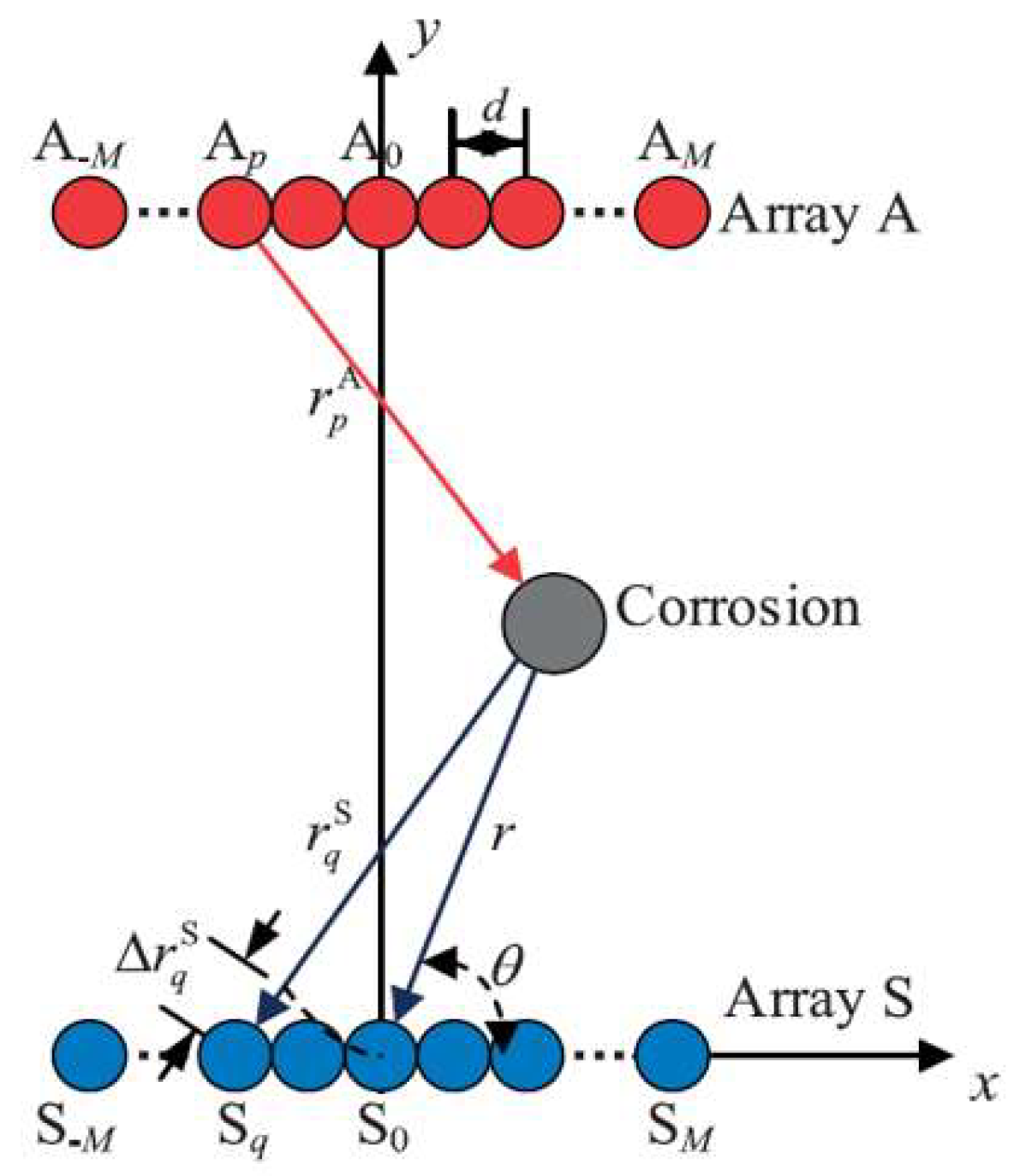
4. Lamb Wave Near-Field Source Location

In the corrosion monitoring of aircraft structures, corrosion damage only accounts for a small part of the whole structure to be monitored, and the rest of the structure is in a non-damage state. Therefore, the whole spatial grid divided by the angle direction can be regarded as a sparse signal. Meanwhile, the states between each angle space of the structure are independent of each other—that is, each column of the observation matrix is irrelevant. Therefore, we can estimate the corrosion angle of aircraft structure by using Lamb wave near-field DOA based on CS. In addition, according to the propagation characteristics of the Lamb wave in an aluminum plate, we use the Lamb wave near-field distance estimation proposed in Chapter 3 to locate the corrosion distance so as to realize the corrosion location in the structure.

The LWNFL method arranges two rows of PZT sensors in the area to be monitored; one row is used to generate excitation signals, and the other is used to receive the sensing signals. Firstly, the excitation sensors generate Lamb waves in turn, which propagate to the corrosion damage and generate scattering. Here, the corrosion damage is regarded as a secondary signal source. The array sensors receive the scattered signals of the corrosion damage, and then Lamb wave near-field DOA estimation based on CS is used to locate the corrosion angle. The Lamb wave near-field distance estimation is used to locate the corrosion distance. Finally, the angle and distance of corrosion estimated by all excitation sensors are arithmetically averaged, and the final location of corrosion damage is obtained. Figure 4 shows the block diagram of the LWNFL.

The sensor arrangement is shown in Figure 5; it consists of two groups of one-dimensional linear arrays, named array A and array S, where array A is the excitation array and array S is the sensor array. The number of sensors in each group is 2M + 1, and each sensor in the array is named from left to right. The excitation sources are A_-M to A_M, and the sensors are S_-M to S_M. The sensor spacing d is taken to be half of the Lamb wave length λ. With the center of the sensor array as the origin and the line of the sensor array as the x-axis, a coordinate system is established, and the polar coordinate of the corrosion damage position is assumed to be (r, θ).

The specific implementation method is as follows: firstly, an excitation sensor in the excitation source array (we use A_P here) generates a narrow band signal $u\left(t\right)e^{j{\omega }_{0}t}$ with center frequency ω₀ and amplitude u(t). According to the Lamb wave near-field model, the received signal X(t) of the sensor array under A_P excitation can be obtained, and X(t) is represented as [x_-M(t), x_-M+1(t),…x_M(t)]^T. According to the received signal x_i(t) (i = −M,…, M) of each sensor, the symmetric covariance vector r_d is constructed. Then, according to Section 2.3, we construct an observation matrix A(θ) containing only angle information and establish the CS model. By solving the CS equation, we can obtain the solution of sparse vector s. The angle corresponding to non-zero elements in sparse vector s is the angle of corrosion (the angle obtained under the excitation of A_p). In order to increase the accuracy, the observation matrix A(θ) divides the space into 900 parts, each of which is 0.2°, so that the angle estimation can be accurate to 0.2°.

After the excitation element A_p is excited, the next excitation element A_p+1 is used for excitation. In the same way, the angle θ^p+1 of corrosion under this excitation source is calculated. This process is repeated until all excitation sensors are excited. Then, the angle data θⁱ obtained under each excitation source are arithmetically averaged to obtain the final corrosion angle θ. The calculation formula is shown in Equation (31):

$$\theta ={\displaystyle \frac{1}{2M+1}}{\displaystyle {\sum }_{i=-M}^M{\theta }^i}$$

(31)

In the next step, after gaining the Lamb wave propagation velocity c and the Lamb wave travel time difference Δt_i, we can calculate the distance r^p (under A_p excitation) according to Equation (29). Similarly, the distance rⁱ (under other excitation source) is calculated in turn, and then the obtained distance data are arithmetic averaged to obtain the final corrosion distance. The calculation formula is as follows:

$$r={\displaystyle \frac{1}{2M+1}}{\displaystyle {\sum }_{i=-M}^M{r}^i}$$

(32)

The angle θ and distance r obtained according to equations (31) and (32) indicate the location of corrosion damage.

5. Experimental Verification

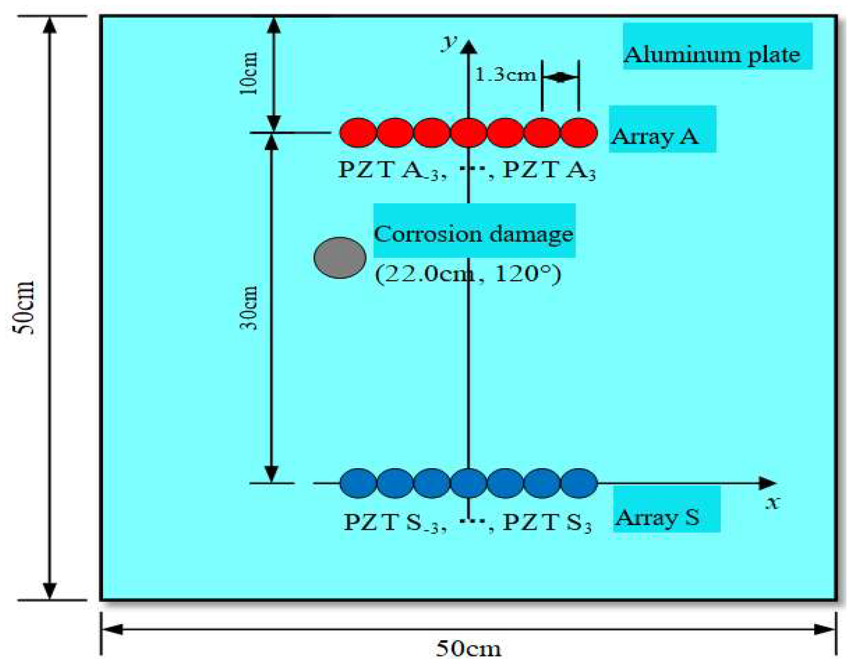
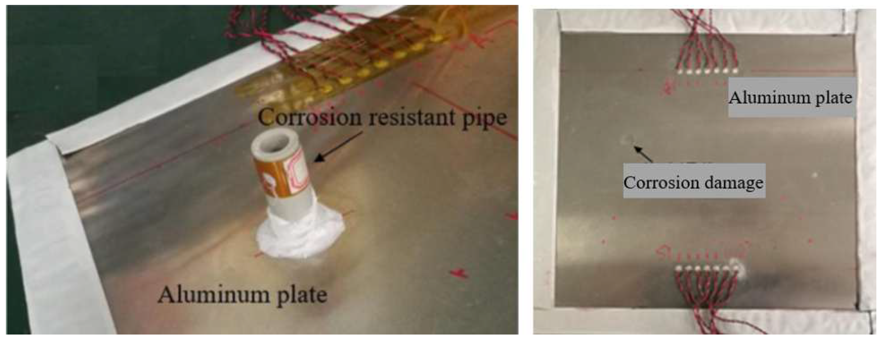
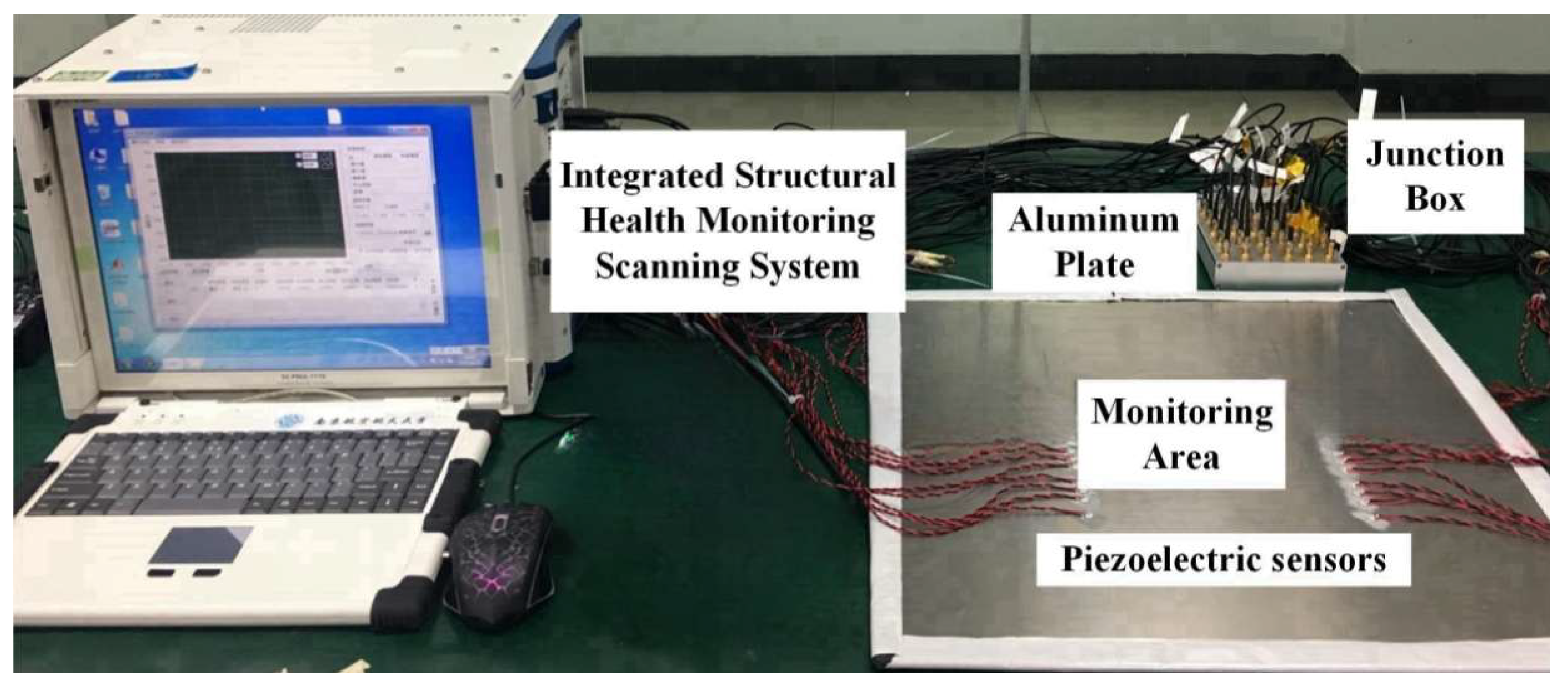
5.1. Experimental Setup

Experiment is carried out on an aviation aluminum plate with a size of 50 cm × 50 cm × 0.3 cm. The PZT sensors are arranged on both sides of the center of the aluminum plate to form two arrays. One array is used to generate excitation signals, named Array A, and the other is used to receive signals, named Array S. Each array has 7 PZT sensors, respectively, and the spacing between adjacent sensors is 1.3 cm. The spacing between the excitation array and sensor array is 30 cm. The excitation array is 10 cm away from the upper side of the aluminum plate, and the sensor array is also 10 cm away from the lower side of the aluminum plate. A coordinate system is established with PZT S₀ as the origin, and corrosion damage is created at the polar coordinate position of (22 cm, 120°) in the monitoring area. The layout diagram of the experiment is shown in Figure 6.

Corrosion in aluminum plates is created by the chemical reaction of dilute hydrochloric acid and aluminum. Before corrosion, the corrosion-resistant tube is fixed at the position to be corroded (22 cm, 120°) with glass glue, and then 20% hydrochloric acid is added to the tube. The corrosion-resistant tube is removed after the chemical reaction is complete, then the waste liquid and residual glass glue on the aluminum plate are cleaned up. Figure 7 shows the devices used for corrosion and the aluminum plate after corrosion.

The scattered signals of corrosion damage can be extracted according to the aluminum plate before and after corrosion. The LWNFL method is used to locate corrosion damage. The flow chart of the experimental method is shown in Figure 8.

In this experiment, the integrated SHM scanning system developed by the authors’ group is used to realize Lamb wave signal excitation and data acquisition. The excitation signals generated by the scanning system are connected to the excitation sensors through the junction box, and the signals received by the sensor array are transmitted to the scanning system through the junction box. Figure 9 shows the scanning equipment, junction box, and aluminum plate used for the experiment. The excitation signal adopts a five-cycle-modified sine wave, and its amplitude is ±70 V. In order to excite the pure A0 mode, the excitation signal frequency in the experiment is set as 70 KHz. The sampling rate is set as 10 MHz, and the signal sampling length is 10,000.

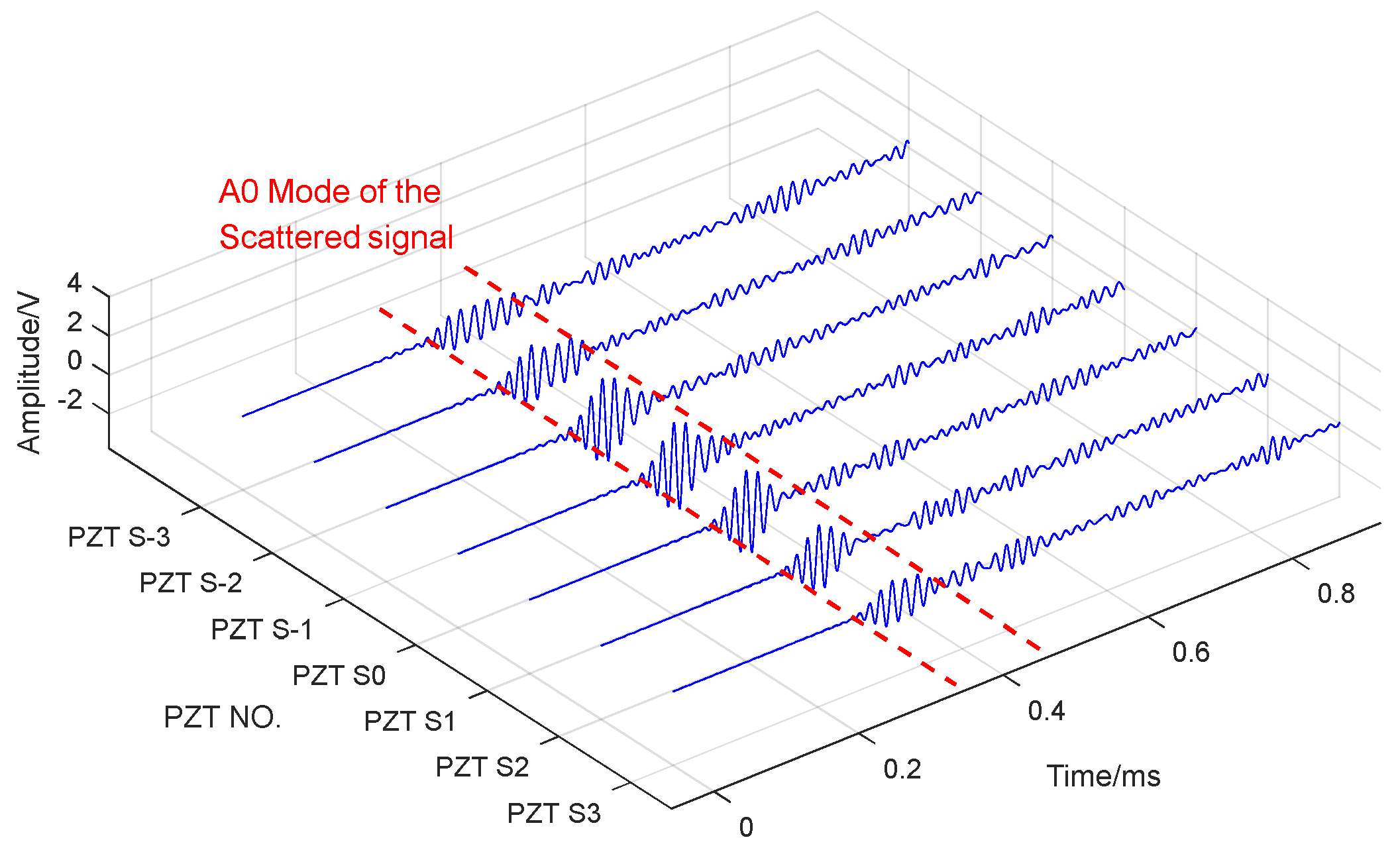
5.2. Experimental Results

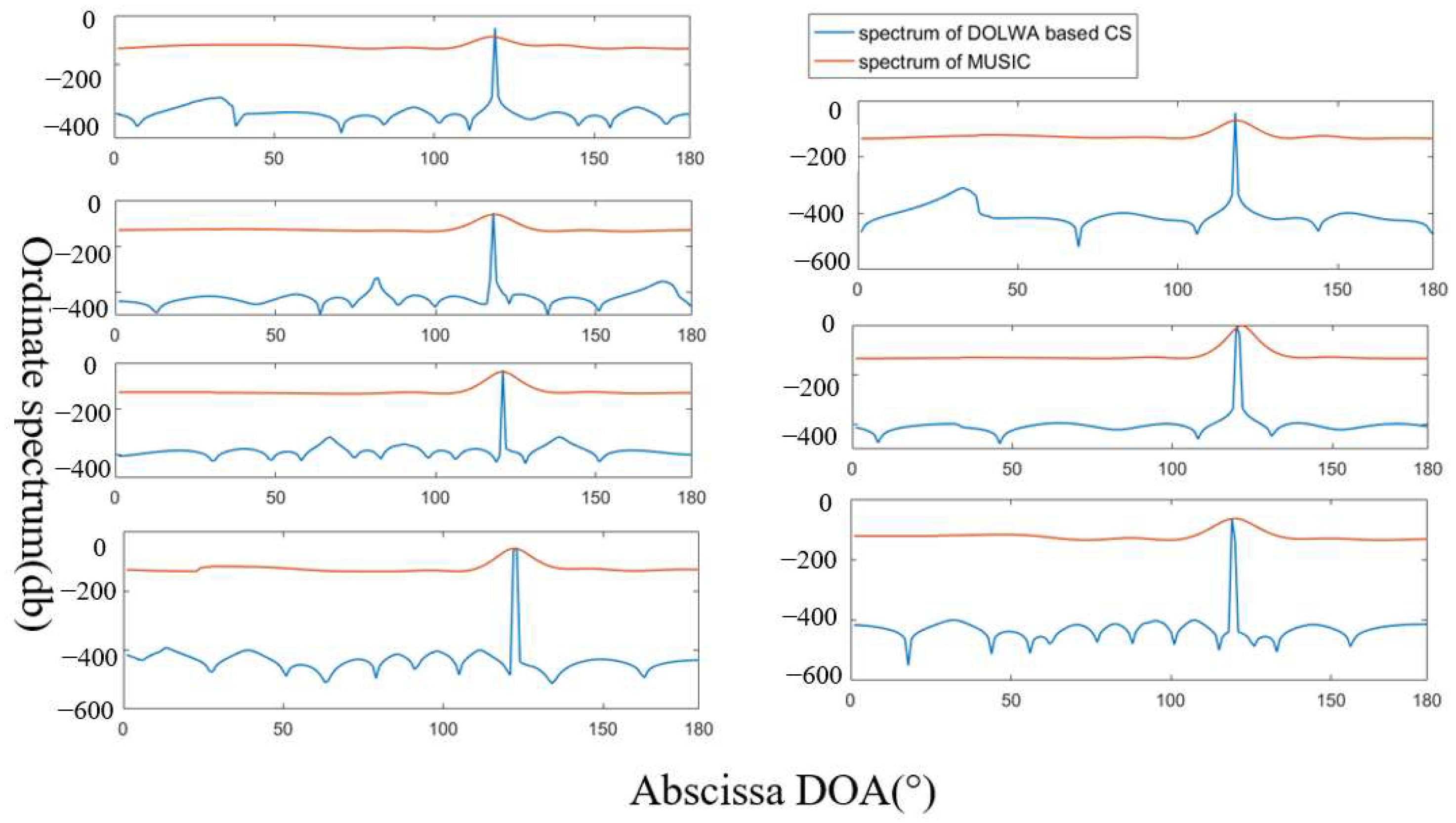
5.2.1. Corrosion Angle Location

The A0 mode of Lamb wave should be extracted from the array’s received signals of corrosion scattering. Here, we use a five-cycle-modified sine wave with a center frequency of 70 kHz as the excitation signal. In this case, the S0 mode is weak in the aluminum plate, and the A0 mode is mainly in the plate. So, the scattering signals are dominated by the A0 mode. Figure 10 shows the received signals of the sensor array under the excitation of PZT A0. As can be seen in the figure, the received signals between 0.24 ms and 0.36 ms belong to the A0 mode of the scattered signals, and the latter part are interference signals. Therefore, we intercept this part of signal data to estimate the angle of corrosion.

The Lamb wave near-field DOA estimation based on CS and MUSIC algorithms is used to estimate the angle direction of corrosion from the intercepted signals. The Lamb wave near-field DOA estimation based on CS sets the space grid unit to 0.2°, and the positioning accuracy is 0.2°. For MUSIC, the search angle step is also set to 0.2°, and the localization accuracy is 0.2°. Seven excitation sensors are separately excited in turn. Figure 11 shows the DOA spectrum obtained by the two methods under different excitation sensors. The angle location results are shown in

Table 1. The corrosion damage angles obtained by the two algorithms under different excitation sources.

Excitation Sensor	Actual Angle	MUSIC Algorithm		Lamb Wave Near-Field DOA Estimation Based on CS
		Localization	Error	Localization	Error
PZT A-3	120°	117.0°	3°	116.6°	3.4°
PZT A-2	120°	122.2°	2.2°	118.2°	1.8°
PZT A-1	120°	123.2°	3.2°	116.8°	3.2°
PZT A0	120°	118.0°	2°	117.6°	2.4°
PZT A1	120°	117.4°	2.6°	118.2°	1.8°
PZT A2	120°	122.2°	2.2°	122.0°	2.0°
PZT A3	120°	122.8°	2.8°	122.2°	2.2°

.

The experimental results show that using the MUSIC algorithm, the maximum angle estimation error is 3.2°, and the minimum angle estimation error is 2°; when using Lamb wave near-field DOA estimation based on CS, the maximum angle estimation error is 3.4° and the minimum angle estimation error is 1.8°. There is little difference in the positioning error between the two methods.

From the perspective of the power spectrum, the height difference between the spectrum peak at 120° (corrosion angle) and the spectrum peak at other angles obtained by the new method is significantly greater than that obtained by MUSIC, and at the angle of 120°, the power spectrum of the new method increases much more steeply than that of MUSIC algorithm. Meanwhile, the spectral width of the new method at 120° is significantly narrower than that of the MUSIC algorithm. This means that the corrosion angle obtained by the new method has a higher resolution and stronger anti-interference ability.

5.2.2. Corrosion Distance Location

Now, we have obtained the angle θ between the corrosion damage and the reference X-axis. According to the characteristics of the aviation aluminum plate, the dispersion curve of Lamb wave on the aluminum plate can be obtained, as shown in Figure 12. Accordingly, it can be shown that the propagation velocity of Lamb wave A0 mode with a center frequency of 70 KHz in the aluminum plate is 2381 m/s. $\Delta t_i$ can be obtained by the difference between the arrival time of the Lamb wave to the reference sensor PZT S0 and the arrival time of the Lamb wave to other sensors PZT Si (i = −3, −2,−1, 1, 2, 3).

Figure 13 shows the schematic diagram of the arrival time of the received signals from PZT S0 and PZT S3 under PZT A0 excitation. A point in the rise stage of the secondary wave peak of the received signal is taken as the arrival sampling point. Here, 0.7 times the peak value of the secondary wave peak is taken. In this case, the Lamb wave arrival times t3 and t0 can be obtained. The Lamb wave arrival time difference Δt₃ can be obtained by t3–t0, and the distance r_0–3 from the corrosion to the reference sensor can be calculated using Equation (29). According to the same method, the Lamb wave arrival time difference Δt_i between the other sensor and the reference sensor can be calculated, and the distance r_0–i from the corrosion damage to the reference sensor can be calculated. The six distance values obtained are averaged as the final corrosion damage distance under the single excitation sensor.

The distance from corrosion damage to the coordinate origin under 7 excitation sensors was calculated, and the results were compared with the results using the MUSIC algorithm.

Table 2. The corrosion damage distances obtained using the two methods under different excitation sources.

Excitation Sensor	Actual Distance	MUSIC		Lamb Wave Near-Field Distance Estimation
		Localization Result	Error	Localization Result	Error
PZT A-3	220 mm	196 mm	24 mm	246 mm	26 mm
PZT A-2	220 mm	240 mm	20 mm	207 mm	13 mm
PZT A-1	220 mm	236 mm	16 mm	239 mm	19 mm
PZT A0	220 mm	201 mm	19 mm	208 mm	12 mm
PZT A1	220 mm	205 mm	15 mm	206 mm	14 mm
PZT A2	220 mm	244 mm	24 mm	200 mm	20 mm
PZT A3	220 mm	191 mm	29 mm	194mm	26 mm

shows the distance positioning results of the two methods.

According to the experimental results, the maximum error and minimum error are 26 mm and 12 mm by using Lamb wave near-field distance estimation. Using the MUSIC algorithm, the maximum error is 29 mm, and the minimum error is 14 mm.

5.2.3. Location Result Analysis

The LWNFL method proposed in this paper uses the average values of angles and distances obtained under multiple excitation sources as the final locating results. The corrosion angles and distances obtained under 7 excitation sensors are numerically averaged, and the location of corrosion damage obtained by the new method is (214.3 mm, 118.8°). It is relatively close to the actual corrosion position (220 mm, 120°), which can realize the accurate positioning of the corrosion.

Table 3. Comparison of corrosion location results.

	Location Results		Error		DOA Power Spectrum
	Angle	Distance	Angle	Distance
MUISC	117.4°	205 mm	2.6°	15 mm	Increases slowly, wider spectrum range, small peak difference at corrosion angle
LWNFL	118.8°	214.3 mm	1.2°	5.7 mm	Increases steeply, narrower spectrum range, small peak difference at corrosion angle

compares the corrosion location results of the LWNFL method and the traditional MUSIC algorithm. Figure 14 shows the actual corrosion location and the corrosion localization results using the two methods.

The experimental results show that the LWNFL method is superior to the traditional MUSIC method in locating corrosion damage of aluminum plate structures in both accuracy and DOA spectrum. This is because the LWNFL method proposed in this paper is used to average the location results under 7 excitations, respectively, so that the locating error of the method is small and the corrosion location can be accurately located. Meanwhile, the noise interference is suppressed by the mathematical method, which makes the LWNFL method more capable of shielding interference and has a higher resolution.

6. Discussion

In order to improve the shortcomings of MUSIC in Lamb wave DOA estimation and realize corrosion monitoring, this study introduces the compressed sensing theory into the Lamb wave near-field array signal model and proposes the LWNFL method. The new proposed method adopts a dual-array sensor arrangement, and it reduces the localization error by averaging the positioning results obtained by multiple excitations. The corrosion location experimental results show that the angle error and the distance error are 1.2° and 5.7 mm, respectively, using the new method. Meanwhile, the DOA spectrum obtained by the new method has a narrow and high lobe at the corrosion angle, which means the new method has a high resolution and good anti-interference. Furthermore, the LWNFL method can monitor multiple sources. In the next step, the authors will carry out research on monitoring multi-damage on a complex structure using this method.

References

1. Alexopoulos, N.D.; Dalakouras, C.J.; Skarvelis, P.; Kourkoulis, S.K. Accelerated corrosion exposure in ultra thin sheets of 2024 aircraft aluminium alloy for GLARE applications. Corros. Sci. 2012, 55, 289–300. [Google Scholar] [CrossRef]
2. Braga, D.F.; Tavares, S.M.O.; Silva, L.F.; Moreira, P.M.G.P.; Castro, P.M. Advanced design for lightweight structures: Review and prospects. Prog. Aerosp. Sci. 2014, 69, 29–39. [Google Scholar] [CrossRef]
3. Ren, Y.Q.; Qiu, L.; Yuan, S.F.; Fang, F. Multi–damage imaging of composite structures under environmental and operational conditions using guided wave and Gaussian mixture model. Smart Mater. Struct. 2019, 28, 115017–115031. [Google Scholar] [CrossRef]
4. Qing, X.L.; Li, W.Z.; Wang, Y.S.; Sun, H. Piezoelectric transducer–based structural health monitoring for aircraft applications. Sensors 2019, 19, 545. [Google Scholar] [CrossRef] [PubMed]
5. Yuan, S.F.; Ren, Y.Q.; Qiu, L.; Mei, H. A multi-response-based wireless impact monitoring network for aircraft composite structures. IEEE Trans. Ind. Electron. 2016, 63, 7712–7722. [Google Scholar] [CrossRef]
6. Bao, Q.; Yuan, S.F.; Guo, F.Y.; Qiu, L. Transmitter beamforming and weighted image fusion-based multiple signal classification algorithm for corrosion monitoring. Struct. Health Monit. 2019, 18, 621–634. [Google Scholar] [CrossRef]
7. Ding, X.; Xu, C.; Deng, M.; Zhao, Y.; Bi, X.; Hu, N. Experimental investigation of the surface corrosion damage in plates based on nonlinear Lamb wave methods. NDT E Int. 2021, 121, 102466. [Google Scholar] [CrossRef]
8. Shang, L.; Zhang, Z.; Tang, F.; Cao, Q.; Pan, H.; Lin, Z. CNN-LSTM hybrid model to promote signal processing of ultrasonic guided lamb waves for damage detection in metallic pipelines. Sensors 2023, 23, 7059. [Google Scholar] [CrossRef] [PubMed]
9. Huang, L.; Luo, Z.; Zeng, L.; Lin, J. Detection and localization of corrosion using the combination information of multiple Lamb wave modes. Ultrasonics 2024, 138, 107246. [Google Scholar] [CrossRef]
10. Pozo, F.; Tibaduiza, D.A.; Vidal, Y. Sensors for structural health monitoring and condition monitoring. Sensors 2021, 21, 1558. [Google Scholar] [CrossRef] [PubMed]
11. O’Leary, D.P. The Direction-of-Arrival Problem: Coming at You. Comput. Sci. Eng. 2003, 5, 60–63. [Google Scholar] [CrossRef]
12. Engholm, M.; Stepinski, T. Direction of arrival estimation of Lamb waves using circular arrays. Struct. Health Monit. 2011, 10, 467–480. [Google Scholar] [CrossRef]
13. Yang, H.; Lee, Y.J.; Lee, S.K. Impact source localization in plate utilizing multiple signal classification. Proc. Inst. Mech. Eng. Part C J. Mech. Eng. Sci. 2013, 227, 703–713. [Google Scholar] [CrossRef]
14. Yuan, S.; Zhong, Y.; Qiu, L.; Wang, Z. Two-dimensional near-field multiple signal classification algorithm-based impact localization. J. Intell. Mater. Syst. Struct. 2015, 26, 703–704. [Google Scholar] [CrossRef]
15. Zhong, Y.; Yuan, S.; Qiu, L. Multi-impact source localisation on aircraft composite structure using uniform linear PZT sensors array. Struct. Infrastruct. Eng. 2015, 11, 310–320. [Google Scholar] [CrossRef]
16. Zhong, Y.; Yuan, S.; Qiu, L. An improved two-dimensional multiple signal classification approach for impact localization on a composite structure. Struct. Health Monit. 2015, 14, 385–401. [Google Scholar] [CrossRef]
17. Zhong, Y.; Yuan, S.; Qiu, L. Multiple damage detection on aircraft composite structures using near-field MUSIC algorithm. Sens. Actuators A Phys. 2014, 214, 234–244. [Google Scholar] [CrossRef]
18. Jalal, B.; Yang, X.; Wu, X.; Long, T.; Sarkar, T.K. Efficient direction-of-arrival estimation method based on variable-step-size LMS algorithm. IEEE Antennas Wirel. Propag. Lett. 2019, 18, 1576–1580. [Google Scholar] [CrossRef]
19. Tang, Y.; Chien, Y.R.; Qian, G. Low complexity error-censoring RLS algorithm for DOA estimation. IEEE Sens. J. 2023, 23, 17237–17244. [Google Scholar] [CrossRef]
20. Zhang, D.; Zhang, Y.; Zheng, G.; Feng, C.; Tang, J. Improved DOA estimation algorithm for co-prime linear arrays using root- MUSIC algorithm. Electron. Lett. 2017, 53, 1277–1279. [Google Scholar] [CrossRef]
21. Tang, B.; Tang, J.; Zhang, Y.; Zheng, Z. Maximum likelihood estimation of DOD and DOA for bistatic MIMO radar. Signal Process. 2013, 93, 1349–1357. [Google Scholar] [CrossRef]
22. Lubeigt, C.; Vincent, F.; Ortega, L.; Vila-Valls, J.; Chaumette, E. Approximate maximum likelihood time-delay estimation for two closely spaced sources. Signal Process. 2023, 210, 109056. [Google Scholar] [CrossRef]
23. Chakrabarty, S.; Habets, E.A. Multi-speaker DOA estimation using deep convolutional networks trained with noise signals. IEEE J. Sel. Top. Signal Process. 2019, 13, 8–21. [Google Scholar] [CrossRef]
24. Xiang, H.; Chen, B.; Yang, T.; Liu, D. Improved de-multipath neural network models with self-paced feature-to-feature learning for DOA estimation in multipath environment. IEEE Trans. Veh. Technol. 2020, 69, 5068–5078. [Google Scholar] [CrossRef]
25. Donoho, D.L. Compressed sensing. IEEE Trans. Inf. Theory 2006, 52, 1289–1306. [Google Scholar] [CrossRef]
26. Candes, E.J.; Tao, T. Decoding by linear programming. IEEE Trans. Theory 2005, 59, 4203–4215. [Google Scholar] [CrossRef]
27. Candes, E.J.; Romberg, J.; Tao, T. Robust uncertainty principles: Exact signal recognition from highly incomplete frequency information. IEEE Trans. Inf. Theory 2006, 52, 489–509. [Google Scholar] [CrossRef]
28. Malioutov, D.M.; Cetin, M.; Willsky, A.S. A sparse signal reconstruct on perspective for source localization with sensor arrays. IEEE Trans. Signal Process. 2005, 53, 3010–3022. [Google Scholar] [CrossRef]
29. Mirza, H.A.; Raja, M.A.Z.; Chaudhary, N.I.; Qureshi, I.M.; Malik, A.N. A robust multi sample compressive sensing technique for DOA estimation using sparse antenna array. IEEE Access 2020, 8, 140848–140861. [Google Scholar] [CrossRef]
30. Srinivas, K.; Ganguly, S.; Kishore, K.P. Performance comparison of reconstruction algorithms in compressive sensing based single snapshot doa estimation. IETE J. Res. 2022, 68, 2876–2884. [Google Scholar] [CrossRef]
31. Hu, B.; Shen, X.; Jiang, M.; Zhao, K. Off-Grid DOA Estimation Based on Compressed Sensing on Multipath Environment. Int. J. Antennas Propag. 2023, 2023, 9315869. [Google Scholar] [CrossRef]
32. Wu, M.; Hao, C. Super-resolution TOA and AOA estimation for OFDM radar systems based on compressed sensing. IEEE Trans. Aerosp. Electron. Syst. 2022, 58, 5730–5740. [Google Scholar] [CrossRef]
33. Liu, L.; Zhang, X.; Chen, P. Compressed sensing-based DOA estimation with antenna phase errors. Electronics 2019, 8, 294. [Google Scholar] [CrossRef]
34. Yan, H.; Chen, T.; Wang, P.; Zhang, L.; Cheng, R.; Bai, Y. A direction-of-arrival estimation algorithm based on compressed sensing and density-based spatial clustering and its application in signal processing of MEMS vector hydrophone. Sensors 2021, 21, 2191. [Google Scholar] [CrossRef]
35. Baraniuk, R.G. A lecture on compressive sensing. IEEE Signal Process. Mag. 2007, 24, 1–9. [Google Scholar] [CrossRef]
36. Tsaig, Y.; Donoho, D.L. Extensions of compressed sensing. Signal Process. 2006, 86, 549–571. [Google Scholar] [CrossRef]
Figure 1. Schematic diagram of near-field Lamb wave signal propagation.
Electronics 14 00907 g001
Figure 2. Lamb wave near-field model based on CS.
Electronics 14 00907 g002
Figure 3. Schematic diagram of the signal source and sensor array distribution.
Electronics 14 00907 g003
Figure 4. Schematic diagram of LWNFL.
Electronics 14 00907 g004
Figure 5. Sensor array layout of LWNFL.
Electronics 14 00907 g005
Figure 6. Schematic diagram of sensor and corrosion position in the experiment.
Electronics 14 00907 g006
Figure 7. Aluminum plate during and after corrosion.
Electronics 14 00907 g007
Figure 8. Flow chart of corrosion location experiment.
Electronics 14 00907 g008
Figure 9. PZT scanning system, junction box, and aluminum plate specimen.
Electronics 14 00907 g009
Figure 10. Lamb wave received by sensor array under PZT A0 excitation.
Electronics 14 00907 g010
Figure 11. DOA spectrum estimated by the two methods under 7 excitation sensors.
Electronics 14 00907 g011
Figure 12. Dispersion curve of the Lamb wave in aluminum plate.
Electronics 14 00907 g012
Figure 13. Schematic of Lamb wave arrival time of PZT S0 and PZT S3 under PZT A0 excitation.
Electronics 14 00907 g013
Figure 14. The actual corrosion localization and the locating results of the two methods.
Electronics 14 00907 g014