Bounded-Error LiDAR Compression for Bandwidth-Efficient Cloud-Edge In-Vehicle Data Transmission

Abstract

Recent advances in autonomous driving have led to an increased use of LiDAR (Light Detection and Ranging) sensors for high-frequency 3D perceptions, resulting in massive data volumes that challenge in-vehicle networks, storage systems, and cloud-edge communications. To address this issue, we propose a bounded-error LiDAR compression framework that enforces a user-defined maximum coordinate deviation (e.g., 2 cm) in the real-world space. Our method combines multiple compression strategies in both axis-wise metric Axis or Euclidean metric L2 (namely, Error-Bounded Huffman Coding (EB-HC), Error-Bounded 3D Compression (EB-3D), and the extended Error-Bounded Huffman Coding with 3D Integration (EB-HC-3D)) with a lossless Huffman coding baseline. By quantizing and grouping point coordinates based on a strict threshold (either axis-wise or Euclidean), our method significantly reduces data size while preserving the geometric fidelity. Experiments on the KITTI dataset demonstrate that, under a 2 cm bounded-error, our single-bin compression reduces the data to 25–35% of their original size, while multi-bin processing can further compress the data to 15–25% of their original volume. An analysis of compression ratios, error metrics, and encoding/decoding speeds shows that our method achieves a substantial data reduction while keeping reconstruction errors within the specified limit. Moreover, runtime profiling indicates that our method is well-suited for deployment on in-vehicle edge devices, thereby enabling scalable cloud-edge cooperation.

1. Introduction

Recent years have witnessed a rapid increase in the use of LiDAR (Light Detection and Ranging) sensors for autonomous driving and advanced driver-assistance systems (ADASs) [1,2]. By emitting laser pulses and measuring their reflections, LiDAR generates high-frequency 3D point clouds with potentially hundreds of thousands or even millions of points per scan. Such dense data streams exert heavy demands on the in-vehicle network, onboard storage resources, and any cloud-edge communication channels [3]. Although modern automotive hardware (e.g., ECUs or embedded GPUs) has progressed to handle certain local computations, naively storing or transmitting voluminous LiDAR data can easily overwhelm bandwidth limits, especially when multiple sensors or vehicles are involved [4,5]. Consequently, it becomes critical to devise an effective compression strategy that both significantly reduces the data size and preserves the essential geometric structure of LiDAR measurements.

Traditionally, many in-vehicle data compression methods have relied on lossless techniques such as Huffman coding [6,7]. While these early solutions can benefit in-vehicle networks, they do not address the specific spatial nature of LiDAR point clouds. As a result, conventional lossless approaches often yield only limited compression for high-frequency point clouds [8]. In recent years, several LiDAR-specific strategies employing octree-based partitioning have demonstrated better efficiency by exploiting the sensor’s physical-space distribution, confirming that designing octree methods around LiDAR’s data traits can enhance compression. Nonetheless, when these methods are treated as purely lossy via bit-depth quantization, they often lack a precise real-world error bound $\le T$. Without controlling $T$, deviations may exceed the LiDAR sensor’s inherent precision, defeating the purpose of high-grade 3D scanning [9]. Conversely, if $T$ is set too conservatively, one may gain negligible compression benefits [10]. To address such constraints, this paper adopts a bounded-error compression scheme that explicitly sets a maximum coordinate deviation $T$ to maintain geometric fidelity while substantially reducing data volume.

Under this bounded-error approach, one could refine the scheme further by assigning finer quantization to high-precision regions (e.g., object edges) and coarser approximations elsewhere, although we do not currently subdivide point clouds in this manner. Even in a uniform configuration, however, guaranteeing no deviation beyond $T$ ensures sufficient accuracy for autonomous-driving tasks without inflating storage or network costs. Based on this concept, we introduce a bounded-error LiDAR compression framework supporting multiple methods, including Huffman coding (as a lossless baseline), Error-Bounded Huffman Coding (EB-HC) (available in both axis-wise (Axis) and Euclidean (L2) variants), Error-Bounded Huffman Coding with 3D Integration (EB-HC-3D) (Axis/L2), and Error-Bounded 3D Compression (EB-3D) (Axis/L2). In practice, each raw point $p=\left(x,y,z\right)$ is approximated by a representative $p_{rep}=\left(x_{\mathrm{rep}},y_{\mathrm{rep}},z_{\mathrm{rep}}\right)$. By quantizing and grouping point coordinates with a strict threshold (either $\max \left(\left|x-x_{\mathrm{rep}}\right|,\left|y-y_{\mathrm{rep}}\right|,\left|z-z_{\mathrm{rep}}\right|\right)$ or Euclidean norm $|p-p_{\mathrm{r}\mathrm{e}\mathrm{p}}{|}_2$), our framework achieves high compression ratios while keeping reconstructed points within $T$ of the originals. Empirical results on the KITTI dataset demonstrate that these methods can often shrink LiDAR data by 70% to 90% (or more), with minimal impact on downstream applications.

Our study aims to (1) propose a controllable-error compression platform tailored for LiDAR data, (2) verify its effectiveness on single-bin and multi-bin scenarios under different threshold settings, and (3) analyze its feasibility in cloud-edge cooperative environments, where large-scale data offloading must remain bandwidth-efficient. Furthermore, we consolidate various bounded-error techniques (encompassing differential coding, Huffman-based entropy, and octree-inspired spatial partitioning) and adapt them to real-time edge hardware constraints. Experimental results confirm that these approaches, particularly EB-HC-3D and EB-3D, achieve a superior trade-off among compression ratio, error bounds, and runtime overhead. Ultimately, by ensuring that point-wise errors remain below LiDAR’s inherent sensing precision, the framework preserves the crucial 3D geometry for autonomous driving tasks and unlocks more scalable cloud-edge cooperation.

The rest of this paper is organized as follows. Section 2 reviews related work on LiDAR compression and cloud-edge integration. Section 3 details our bounded-error methods along with Axis and L2 error measures. Next, we describe our experimental setup, specifying the datasets, error thresholds, and hardware. We then present and discuss the results, including compression ratio, error analysis, and runtime performance, in Section 4. Finally, Section 5 concludes by summarizing our contributions and outlining opportunities for further refinements of bounded-error LiDAR compression in autonomous driving.

2. Related Works

LiDAR sensors have proven vital in autonomous driving and ADAS for their ability to capture high-density 3D scans of surrounding environments in real time [11,12]. Although standard data packaging formats (such as bin, pcap, and ROS bag) are convenient for logging and transferring raw sensor outputs, they can rapidly saturate on-vehicle network and storage resources [13]. A common approach is to perform preliminary compression or processing at the edge, thereby reducing the volume of data that must be uploaded for tasks such as high-definition map creation or large-scale model training [14]. Nevertheless, LiDAR streams can reach tens or even hundreds of megabytes per second, meaning that designing a robust compression method (one that preserves essential geometric detail) remains a persistent challenge [15]. A variety of LiDAR compression techniques have consequently emerged. Some code-based (signal-processing-based) methods rely on bit-level transformations or learned entropy coding [16,17], including predictive + arithmetic coding that can reduce bin size to roughly 12% of the original, or hierarchical grid modeling for large-scale streaming [18]. Meanwhile, neural or range-image strategies transform LiDAR data into 2D depth (range) images and employ RNNs (recurrent neural networks) or delta-based transforms to lower bitrates by 30% to 35%, thus easing bandwidth demands before cloud fusion [19,20].

Other techniques exploit LiDAR’s 3D geometry by octree partitioning. Compression results with octree-based methods [21] to neural-entropy-driven approaches like OctSqueeze [22] and multi-sweep expansions save 15% to 35% overall [23]. Some works adapt MPEG G-PCC for automotive LiDAR, improving geometry coding for spinning scans [24] or incorporating rate-distortion optimization [25]. Finally, Google’s Draco, originally for 3D meshes, can encode LiDAR via geometry transforms or spherical projection [26], while semantic segmentation further discards non-critical points for real-time compression [27]. Although each approach balances trade-offs in complexity, error control, and ratio gains, all share the goal of delivering an efficient edge-cloud pipeline capable of handling LiDAR’s data-intensive demands in autonomous driving.

Bounded-error compression has proven effective in IoT and industrial sensing, where small deviations can generate major reductions in network overhead and power consumption. In one study, a 1% error tolerance reduced sensor transmission by over 55% and halved energy usage [28]. Another effort demonstrated that even with 0.5–2% allowed error, sensors could save up to 70% of their communication energy [29]. Moreover, edge-based filtering can slash communication costs by as much as 88%, making real-time operations viable in resource-limited scenarios [30]. Despite these achievements in 1D or 2D sensor data, 3D LiDAR demands stricter precision, hence the need for more robust bounded-error approaches in autonomous driving. A recent study enforces an error bound across dense and sparse LiDAR regions [9]. In parallel, our approach extends this concept by supporting either axis-wise or L2 distance constraints, ensuring greater flexibility for various LiDAR applications.

Despite these advances, several gaps remain. First, the automotive scenario specifically demands a balance between high LiDAR accuracy and bandwidth constraints on in-vehicle or V2X links. Second, while certain works mention bounding errors in 3D, there is no widely adopted framework that lets users rigorously set and enforce a real-world maximum error limit across an entire LiDAR dataset. Third, few comparative studies exist that evaluate multiple bounded-error point cloud algorithms side by side under realistic driving conditions. Motivated by these gaps, this paper proposes a unified bounded-error LiDAR compression architecture that enables a user-defined coordinate deviation limit, aligning sensor precision with network-efficiency goals in autonomous vehicles.

3. Proposed Bounded-Error Compression Methods

This section introduces a unified LiDAR compression framework that enforces a user-specified geometric error bound, $T$, in real-world coordinates (either via an axis-wise metric or a Euclidean L2 metric). The framework comprises seven different methods, of which the first is a lossless Huffman baseline, and the remaining six apply bounded-error constraints in distinct ways. Specifically, we incorporate Huffman (as a baseline), EB-HC (Axis/L2), EB-3D (Axis/L2), and EB-HC-3D (Axis/L2). All but Huffman allow the user to preset a strict maximum coordinate deviation $T$ (for example, 2 cm) that cannot be exceeded when reconstructing the compressed point cloud. We divide this section into five parts. Section 3.1 explains the concept of bounded-error quantization and the two distance metrics used; Section 3.2 describes Huffman coding as the lossless reference; Section 3.3 discusses EB-HC; Section 3.4 focuses on EB-3D; and Section 3.5 introduces EB-HC-3D.

3.1. Bounded-Error Quantization and Error Metrics

Unlike conventional LiDAR compression that might rely solely on bit-depth quantization or purely lossless entropy coding, a bounded-error approach allows the user to specify an absolute geometric threshold $T$. In practice, each raw point $p=\left(x,y,z\right)$ is approximated by a representative $p_{rep}=\left(x_{\mathrm{rep}},y_{\mathrm{rep}},z_{\mathrm{rep}}\right)$ that satisfies one of the following two constraints:

$$\max \left(\left|x-x_{\mathrm{rep}}\right|,\left|y-y_{\mathrm{rep}}\right|,\left|z-z_{\mathrm{rep}}\right|\right)\le T$$

(1)

$${‖p-p_{rep}‖}_2=\sqrt{{\left(x-x_{\mathrm{rep}}\right)}^2+{\left(y-y_{\mathrm{rep}}\right)}^2+{\left(z-z_{\mathrm{rep}}\right)}^2}\le T$$

(2)

Equation (1) indicates the axis-wise bound, while Equation (2) enforces the Euclidean L2 bound. This threshold T is chosen to be near or above the sensor’s inherent precision, ensuring that no application-critical geometry is lost despite a potentially aggressive reduction in data volume. The overall process typically begins by quantizing the raw floating-point coordinates with a chosen scale factor α. Once the points are quantized, subsequent steps cluster or partition them so that each cluster’s representative remains within the specified bound, whether along each axis or with respect to the 3D Euclidean metric.

3.2. Huffman Coding (Lossless Baseline)

Huffman coding serves as a baseline method with zero geometric loss relative to the quantized coordinates. After the point coordinates have been converted into integers, the three dimensions for each point are serialized into a sequence of bytes and then processed by a standard Huffman encoder. This encoder calculates the frequency of each byte value, constructs a Huffman tree, and replaces frequent symbols with shorter codes, thus compressing the data without introducing any further error. For example, if the byte “120” appears most frequently in the stream, Huffman might encode it with just “0”, while a rarer byte requires a longer pattern such as “1011”. Decoding reverses the process, reconstructing the original bytes from Huffman codes and finally converting integers back to (x, y, z). While it preserves full fidelity at the quantized resolution, Huffman coding alone generally produces only limited compression for large, high-frequency LiDAR datasets. Nevertheless, it serves as a valuable reference for measuring how much additional reduction can be gained by allowing a small bounded-error in other methods.

3.3. EB-HC (Axis/L2)

EB-HC merges or clusters nearby quantized coordinates so that no merged group’s representative deviates from any point in that group by more than $T$. The method operates separately for the axis-based bound and for the Euclidean (L2) bound. Under the axis-based approach, the algorithm sorts integer coordinates along each dimension and merges values whose differences do not exceed a threshold $\delta$. As shown in Equation (3),

$${\delta }_{axis}=⌊{\displaystyle \frac{\mathrm{T}\times \mathsf{\alpha }}{\mathrm{u}\mathrm{n}\mathrm{i}\mathrm{t}\text{\_}\mathrm{s}\mathrm{c}\mathrm{a}\mathrm{l}\mathrm{e}}}⌋$$

(3)

where $T$ is the user-specified error bound (e.g., in centimeters), α is the quantization scale factor, and unit_scale covers any additional unit conversion. Each merged cluster then adopts a single “common representative”.

Meanwhile, the L2-based variant must ensure that the 3D Euclidean distance between any point and its representative is at most T. One practical way is to adjust the same δ by $\sqrt{3}$ to cover the worst-case diagonal offset. For instance, one might set

$${\delta }_{L2}={\displaystyle \frac{T\times \mathsf{\alpha }}{unit\text{\_}scale\sqrt{3}}}$$

(4)

so that the final approximations respect the L2-norm bound in Equation (2). In some implementations, this can also be enforced by a direct Euclidean check on each cluster or subtree.

Regardless of whether ${\delta }_{axis}$ or ${\delta }_{L2}$ is used, EB-HC merges nearby integer coordinates into fewer unique values, then compresses those representative values (and mapping information) via Huffman coding. Because EB-HC relies on dimension-wise or cluster-based merging (rather than a full 3D subdivision), it typically runs in O(N log N) time, dominated by the sorting phase.

Algorithm 1 EB-HC illustrates the EB-HC pipeline in detail. Step 1 handles optional preprocessing or coordinate normalization. Step 2 shows how the algorithm partitions the input points using either an axis-wise or a Euclidean threshold $\delta$. Each partitioned group then selects a single representative, as shown in Step 3, replacing all points in that group with one symbol. Finally, Step 4 applies Huffman coding to these representatives, and Step 5 combines them into the compressed bitstream $C_{\mathrm{EB}\text{-}\mathrm{HC}}$. In either axis-based or Euclidean mode, this procedure guarantees that no point in a cluster differs from its representative by more than $\delta$. Consequently, the axis branch enforces Equation (5), while the Euclidean branch uses Equation (6), both of which align with the bounded-error discussion in this subsection. Note that, after Huffman decoding the EB-HC stream, the recovered data include both the cluster representatives and the mapping that associates each original point with its corresponding representative. The extra processing step involves using this mapping to reassign each point to its cluster value, thereby reconstructing the point cloud while ensuring that the reconstruction error remains within the specified bound T.

$$\mathrm{m}\mathrm{a}\mathrm{x}\left(\left|x_i-x_j\right|,\left|y_i-y_j\right|,\left|z_i-z_j\right|\right)\le {\delta }_{axis}$$

(5)

$$\sqrt{{\left(x_i-x_j\right)}^2+{\left(y_i-y_j\right)}^2+{\left(z_i-z_j\right)}^2}\le {\delta }_{L2}$$

(6)

Algorithm 1. EB-HC

Require:  A set of LiDAR points $\mathrm{P}=\{\left(x_i,y_i,z_i\right)$$\}{\displaystyle \genfrac{}{}{0pt}{}{N}{i=1}}$, user-specified threshold δ > 0, and mode ∈ {Axis, L2}

Ensure:   A compressed bitstream $C_{EB-HC}$

1: Step 1: Preprocessing (optional). 2: Optionally quantize or normalize point coordinates if floating precision is excessive. 3: Step 2: Clustering 4: if mode = Axis then 5:  Partition P into clusters such that $max(\left|x_i-x_j\right|,\left|y_i-y_j\right|,\left|z_i-z_j\right|) \le \delta$. 6: else if mode = L2 7:  Partition P into clusters such that $\sqrt{\left({\left(x_i-x_j\right)}^2+{\left(y_i-y_j\right)}^2+{\left(z_i-z_j\right)}^2\right)}\le \delta$. 8: end if 9: Step 3: Representative Selection. 10: For each cluster ${\mathcal{G}}_{\mathcal{k}}$ do 11:  Choose a single representative $r_k$  12:  Replace all points in ${\mathcal{G}}_{\mathcal{k}}$ with the single symbol $r_k$. 13: end for 14: Step 4: Huffman Encoding. 15: Build a frequency table for all representatives $\{r_k$}. 16: Construct a Huffman tree from these frequencies. 17: Encode each $r_k$ to a variable-length bitstring via the Huffman code. 18: Step 5: Output. 19: Combine the Huffman-encoded symbols and minimal metadata into $C_{EB-HC}$. 20: return $C_{EB-HC}$

3.4. EB-3D (Axis/L2)

EB-3D applies a hierarchical subdivision of the 3D domain, halving along each axis in a recursive manner. Starting with the entire point set, the algorithm computes a center, checks whether all points lie within $T$ (as either in Equation (1) or Equation (2)), and encodes the set as a single leaf node if the error bound is satisfied; otherwise, it subdivides the space into eight octants. Each subdivision repeats until each group of points can be approximated by one center with coordinate deviations ≤ $T$. This process generates a tree of nodes, each storing a small occupancy mask (indicating which of the eight children are nonempty) and a representative center for each leaf. Because many LiDAR scenes contain expansive regions of relatively uniform or empty space, EB-3D can yield high compression ratios by assigning a single representative to large subvolumes. Reconstructing points then involves traversing the encoded tree, identifying leaf nodes, and retrieving their stored centers. Although creating and encoding an octree can be more computationally involved than EB-HC, it excels when the point cloud is large and exhibits significant spatial regularities.

Algorithm 2 EB-3D shows the detailed pseudo-code for EB-3D. In a traditional octree, one typically specifies a fixed maximum depth or resolution beforehand, causing uniform subdivision regardless of local data variation. By contrast, EB-3D halts subdivision in any node whose bounding error ϵ does not exceed $\delta$. Note that in practice, $\delta$ and the user-specified $T$ serve the same role of bounding coordinate deviations, but $\delta$ may be scaled or otherwise adjusted to match implementation details (e.g., quantization). For instance, Equation (3) or Equation (4) illustrates how $\delta$ can be derived from $T$ in a quantized setting. Once the local error is low enough to meet $\delta$, no further splitting is required, so each leaf node merely stores a single representative coordinate rather than all the points it contains. This strategy naturally respects the specified bounded-error criterion while avoiding excessive subdivisions in regions of relative uniformity.

Algorithm 2. EB-3D

Require: A set of LiDAR points $P=\{\left(x_i,y_i,z_i\right){\}}_{i=1}^N$; threshold $\delta >0$; mode $\in \{\mathrm{Axis}, \mathrm{L}2\}; \mathrm{maximum} \mathrm{depth} d_{max}$

Ensure: An octree-based compressed representation $C_{EB-3D}$

1: Step 1: Global Bounding Box. 2: Compute bounding box $\left(x_{min},x_{max}\right),\left(y_{min},y_{max}\right),\left(z_{min},z_{max}\right)$ for P. 3: Let root be the octree’s root node covering this bounding box. 4: Step 2: BuildOctree(root, P, 0). 5:  Store all point indices in root. 6:  Recursively process: 7:  function BuildOctree$\left(N_{node},S_{pts},depth\right)$: 8:  (a) Compute representative r (e.g., centroid of $S_{pts}$). 9:  (b) Evaluate error ε (axis-wise or L2). 10: if  $\mathsf{\epsilon } \le \mathsf{\delta } \mathrm{or} \mathrm{depth} \ge d_{max}$ then 11:  Mark $N_{node}$ as LEAF, store r as leaf coordinate. 12:  return 13: end if  14:  (c) Subdivide bounding box into 8 octants; create child nodes $C_i$. 15:  (d) For each point p in $S_{pts }$, assign p to the corresponding $C_i$. 16:  (e) For each nonempty child $C_i$, call BuildOctree. 17: Step 3: Octree Serialization. 18: Record representatives at leaf nodes + minimal structural info for internal splits. 19: Step 4: Output.  20: Final octree data is $C_{EB-3D}$. 21: return  $C_{EB-3D}$

3.5. EB-HC-3D (Axis/L2)

EB-HC-3D integrates hierarchical subdivision and clustering into a single pipeline, enforcing the chosen bounded-error criterion at each step while additionally applying Huffman coding. It begins by building an EB-3D octree (as discussed in Section 3.4), then encodes each leaf’s representative data in a Huffman-friendly symbol stream rather than storing a single center coordinate. This design can often provide further compression gains, particularly in nonuniform LiDAR distributions, because it simultaneously exploits local redundancy and hierarchical spatial structure.

Algorithm 3 EB-HC-3D illustrates the EB-HC-3D procedure. In Step 1, the algorithm constructs a complete EB-3D octree, halting subdivision in any node whose bounding error ϵ does not exceed $\delta$. Here, $\delta$ corresponds to the user-specified $T$ (see Equation (3) or Equation (4) for a possible conversion). Next, Step 2 gathers all leaf nodes, each storing a representative $r_{{\mathcal{l}}_i}$. Step 3 then applies Huffman coding to these leaf representatives, building a frequency table and generating variable-length bit patterns. Finally, Step 4 packages both the octree structure (indicating which nodes are leaves versus internal splits) and the Huffman-encoded symbols into a compressed bitstream $C_{\mathrm{EB}\text{-}\mathrm{HC}\text{-}3\mathrm{D}}$.

As with EB-3D, the user may enforce either Equation (1) or Equation (2) at each subdivision step, ensuring the maximum coordinate discrepancy remains bounded per-axis (Axis mode) or in Euclidean norm (L2 mode). By additionally compressing leaf descriptors, child masks, and representative offsets via Huffman, EB-HC-3D can reduce data volume more aggressively than a pure octree. Meanwhile, the decoder’s reconstruction process respects the same threshold $T$ throughout, guaranteeing that every recovered point lies within the specified error bound. In terms of runtime, building and traversing the octree typically requires O(N × depth) operations, where N is the number of points and depth depends on how often the space must be subdivided to meet $\delta$. In practice, EB-HC-3D shares the octree’s complexity of O(N × depth), plus additional overhead for generating and applying Huffman codes, which typically remains manageable unless the octree is extremely deep or the data volume is massive.

Algorithm 3. EB-HC-3D

Require: A set of LiDAR points P; threshold $\delta$; mode ∈ {Axis, L2}; maximum depth $d_{max}$  Ensure: A final compressed bitstream $C_{EB-HC-3D}$ 1: Step 1: Build the Octree (EB-3D). 2: Compute bounding box, create root, and run BuildEB3D to form a complete octree with leaves satisfying the error threshold. 3: Step 2: Leaf Representatives as Symbols.  4: Gather leaf nodes $\{l_1,l_2,\dots$} each storing representative $r_{l_i}$. 5: Build a frequency table for $\{r_{l_i}$}. 6: Step 3: Huffman Coding of Representatives.  7: Construct a Huffman tree based on frequencies of $r_{l_i}$. 8: Encode each leaf representative into a bit pattern. 9: Step 4: Final Packaging. 10: Combine: 11:  (a) The octree structure (which nodes are leaves/splits) 12:  (b) Huffman-encoded leaf representatives 13: Form $C_{EB-HC-3D}$. 14: return  $C_{EB-HC-3D}$

3.6. Summary of Proposed Methods

We have introduced seven distinct methods under our bounded-error compression framework, ranging from the purely lossless Huffman baseline to advanced combinations of clustering, octree partitioning, and Huffman encoding.

Table 1. Comparison of proposed methods.

Method	Key Idea	Time Complexity
Huffman	Frequency-based byte encoding (baseline)	$\mathrm{O}\left(N\right)$
EB-HC (Axis)	Merge integer coords along x, y, z + Huffman	$\mathrm{O}\left(N\log N\right)$
EB-HC (L2)	Merge integer coords in 3D distance + Huffman	$\mathrm{O}\left(N\log N\right)$
EB-3D (Axis)	Octree subdivision (per dimension)	$\mathrm{O}\left(N\times \mathrm{depth}\right)$
EB-3D (L2)	Octree subdivision (radial check)	$O\left(N\times \mathrm{depth}\right)$
EB-HC-3D (Axis)	Combine octree + Huffman (axis-based)	$O\left(N\times \mathrm{depth}\right)$
EB-HC-3D (L2)	Combine octree + Huffman (L2-based)	$O\left(N\times \mathrm{depth}\right)$

compares these methods side by side, focusing on each approach’s core idea and typical computational cost. By varying the metric used for bounding errors (Axis versus L2), the partitioning scheme, and whether leaf data are directly stored or Huffman-encoded, these methods accommodate a wide spectrum of trade-offs in compression ratio, error fidelity, and runtime overhead.

4. Evaluation

In this chapter, we present a comprehensive evaluation of our bounded-error LiDAR compression framework. Our experimental analysis is organized into several sections. First, we introduce the KITTI dataset and describe its key characteristics, which make it an ideal testbed for evaluating LiDAR compression in real-world driving scenarios. Next, we detail our evaluation metrics and error settings, where the reconstruction error threshold T varies from 0.25 cm to 10 cm in increments of 0.25 cm. The performance is assessed in terms of compression ratio, encoding/decoding runtime, and reconstruction error measured by both mean and maximum axis-wise and Euclidean (L2) errors.

We then compare the performance of the different compression methods in Section 4.3, including the overall compression performance (such as runtime data) across various methods and error thresholds, as well as the impact of using axis-wise versus L2 error metrics. Section 4.4 discusses the implications of our findings for cloud-edge data transmission, particularly evaluating the real-time feasibility of the methods on typical in-vehicle hardware.

4.1. Dataset Introduction

In this study, we evaluate our bounded-error LiDAR compression framework using data from the KITTI dataset (a widely recognized benchmark in autonomous driving research) [31]. KITTI provides a rich collection of sensor data recorded under real-world driving conditions, including 3D LiDAR point clouds, stereo images, and GPS/IMU measurements. For our evaluation, we exclusively employ the raw LiDAR point clouds provided in binary (bin) format.

Each bin file contains a single LiDAR scan acquired by a 64-beam Velodyne sensor (Velodyne, San Jose, CA, USA), where each scan typically comprises approximately 100,000 points. Every point is represented by a set of four floating-point values corresponding to the x, y, and z coordinates and the reflectivity. Given that the LiDAR sensor operates at 10 Hz, each bin file represents approximately 0.1 s of data.

To ensure that our evaluation captures a broad range of real-world scenarios, we selected sequences from several distinct environments provided by KITTI. Specifically, our experiments include scenes categorized as City, Residential, Road, Campus, and Person. This diverse selection allows us to assess the performance and robustness of our compression framework under various operating conditions and scene complexities.

4.2. Evaluation Metrics and Error Settings

Our evaluation of the compression framework is based on five primary performance indicators that together offer a comprehensive view of its effectiveness. First, we assess the compression efficiency by defining the compression ratio (CR) as the ratio of the number of bits in the compressed bitstream ($c_{bits}$) to that of the raw quantized data ($raw\text{\_}bits$). This metric is expressed mathematically as

$$CR={\displaystyle \frac{c_{bits}}{ra\mathrm{w}\text{\_}\mathrm{b}\mathrm{i}\mathrm{t}\mathrm{s}}}$$

(7)

A lower value of CR indicates that the method achieves a higher degree of compression, which is crucial for reducing storage requirements and transmission bandwidth. In addition to compression efficiency, we measure the computational overhead by recording the encoding time ($t_{enc}$) and decoding time ($t_{dec}$), both reported in seconds. These timing metrics help determine whether the compression and decompression processes can be performed in real time on edge devices; a method that achieves excellent compression but requires excessive processing time may not be suitable for in-vehicle applications.

The fidelity of the reconstructed point cloud is quantified using two error metrics. For an original point $p=\left(x,y,z\right)$ and its reconstruction $\widehat{p}=\left(\widehat{x},\widehat{y},\widehat{z}\right)$, the first metric (the axis-wise error) is defined as the maximum absolute deviation along any coordinate:

$$e_{axis}\left(p,\widehat{p}\right)=\max \{\left|x-\widehat{x}\right|,\left|y-\widehat{y}\right|,\left|z-\widehat{z}\right|\}$$

(8)

Both the mean and maximum values of $e_{axis}$ are computed over the entire point cloud. The second metric, the Euclidean (L2) error, provides an overall measure of the pointwise deviation and is defined as

$$e_{L2}\left(p,\widehat{p}\right)=|p-\widehat{p}{|}_2$$

(9)

Again, both the mean and maximum $e_{L2}\left(p,\widehat{p}\right)$ errors are calculated across the dataset. The error threshold $T$ represents the maximum allowable deviation in real-world coordinates between the original and reconstructed points. In our experiments, $T$ is varied from 0.25 cm up to 10 cm in increments of 0.25 cm, thereby providing a detailed performance profile at 0.25 cm bins. Although the KITTI’s Velodyne sensor (Velodyne, San Jose, CA, USA) typically achieves an accuracy of approximately 2 cm, extending the threshold to 10 cm allows us to explore the trade-off between compression efficiency and reconstruction fidelity over a broader range. This extended range is particularly useful for applications where a slight degradation in geometric precision is acceptable in exchange for significantly reduced data volumes and lower bandwidth requirements for cloud-edge data transmission.

To further characterize reconstruction quality, we additionally incorporate the Chamfer Distance (CD) and the Occupancy Intersection-over-Union (IoU), which focus on local and global completeness, respectively. Chamfer Distance measures the average bidirectional nearest-neighbor distance between two point sets (e.g., original and reconstructed surfaces) and is formulated as follows. For a ground-truth set P and a reconstructed set Q,

$$\mathrm{CD}\left(P,Q\right)={\displaystyle \frac{1}{\left|P\right|}}{\displaystyle \sum _{p\in P}}\underset{q\in Q}{\min }{‖p-q‖}_2+{\displaystyle \frac{1}{\left|Q\right|}}{\displaystyle \sum _{q\in Q}}\underset{p\in P}{\min }{‖q-p‖}_2$$

(10)

A lower CD indicates that every local region of the reconstructed shape lies close to the ground-truth surface and vice versa, implying minimal small-scale discrepancies [32,33]. By contrast, if fine details are lost or distorted, the nearest-neighbor distances become larger, increasing Chamfer Distance.

While Chamfer Distance captures local surface fidelity, Occupancy IoU measures global shape completeness by comparing how much volume is shared between the ground-truth and reconstructed 3D shapes. Concretely, after voxelizing each shape, let V(P) and V(Q) represent the sets of occupied voxels. Occupancy IoU is then

$$\mathrm{IoU}\left(P,Q\right)={\displaystyle \frac{\left|V\left(P\right)\cap V\left(Q\right)\right|}{\left|V\left(P\right)\cup V\left(Q\right)\right|}}$$

(11)

An IoU of 1.0 implies the two volumes match perfectly, whereas 0 means no overlap [34,35]. We typically use a fixed-resolution grid to capture large-scale omissions or extraneous parts. Higher IoU thus indicates more complete volumetric coverage of the object’s structure, complementing the local perspective offered by Chamfer Distance.

The seven metrics discussed—CR, encoding/decoding times, axis-wise/L2 errors, Chamfer Distance, and Occupancy IoU—together offer a multidimensional view of how effectively each compression strategy preserves LiDAR point cloud geometry under practical bandwidth and latency constraints.

Table 2. Summary of evaluation metric symbols and definitions.

Symbol	Definition
CR	Compression ratio, defined as the ratio of the number of bits in the compressed bitstream to that of the raw quantized data.
$t_{enc}$	Encoding time, measured in seconds. This is the time required to compress a point cloud.
$t_{dec}$	Decoding time, measured in seconds. This is the time required to decompress the data.
$e_{axis}\left(p,\widehat{p}\right)$	Axis-wise error, defined as the maximum absolute deviation along any coordinate between an original point $p=\left(x,y,z\right)$ and its reconstruction $\widehat{p}=\left(\widehat{x},\widehat{y},\widehat{z}\right)$.
$e_{L2}\left(p,\widehat{p}\right)$	Euclidean (L2) error, defined as the Euclidean distance between the original point $p$ and its reconstruction $\widehat{ p}$.
CD	A local geometric completeness metric: $\mathrm{CD}\left(P,Q\right)={\displaystyle \frac{1}{\left|P\right|}}{\displaystyle \sum _{p\in P}}\underset{q\in Q}{\min }{‖p-q‖}_2+{\displaystyle \frac{1}{\left|Q\right|}}{\displaystyle \sum _{q\in Q}}\underset{p\in P}{\min }{‖q-p‖}_2.$ A lower CD indicates fewer small-scale errors.
Occupancy IoU	A global volumetric completeness metric: $\mathrm{IoU}\left(P,Q\right)={\displaystyle \frac{\left|V\left(P\right)\cap V\left(Q\right)\right|}{\left|V\left(P\right)\cup V\left(Q\right)\right|}}$. A higher IoU indicates better overall coverage

summarizes all these indicators.

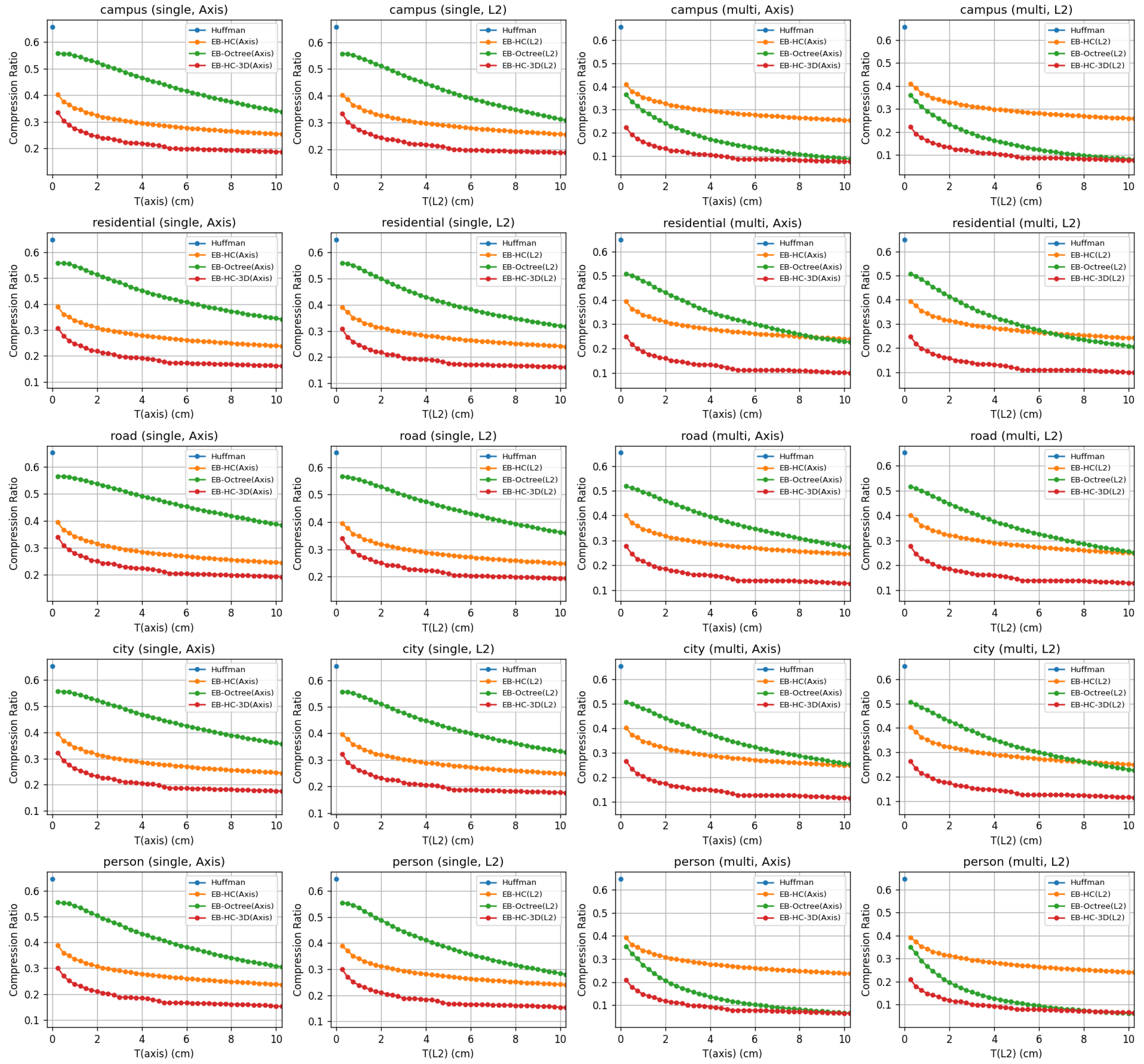
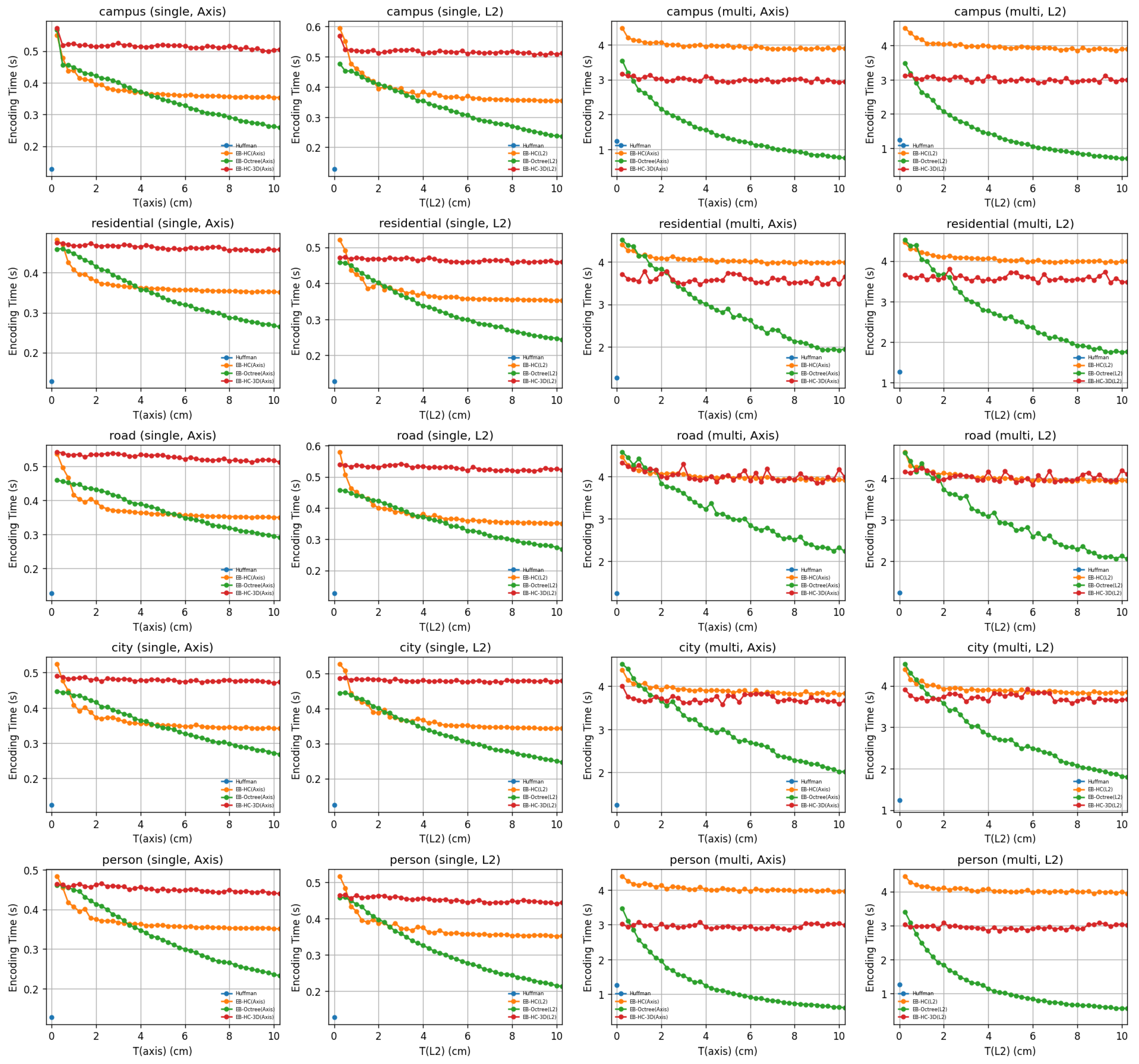
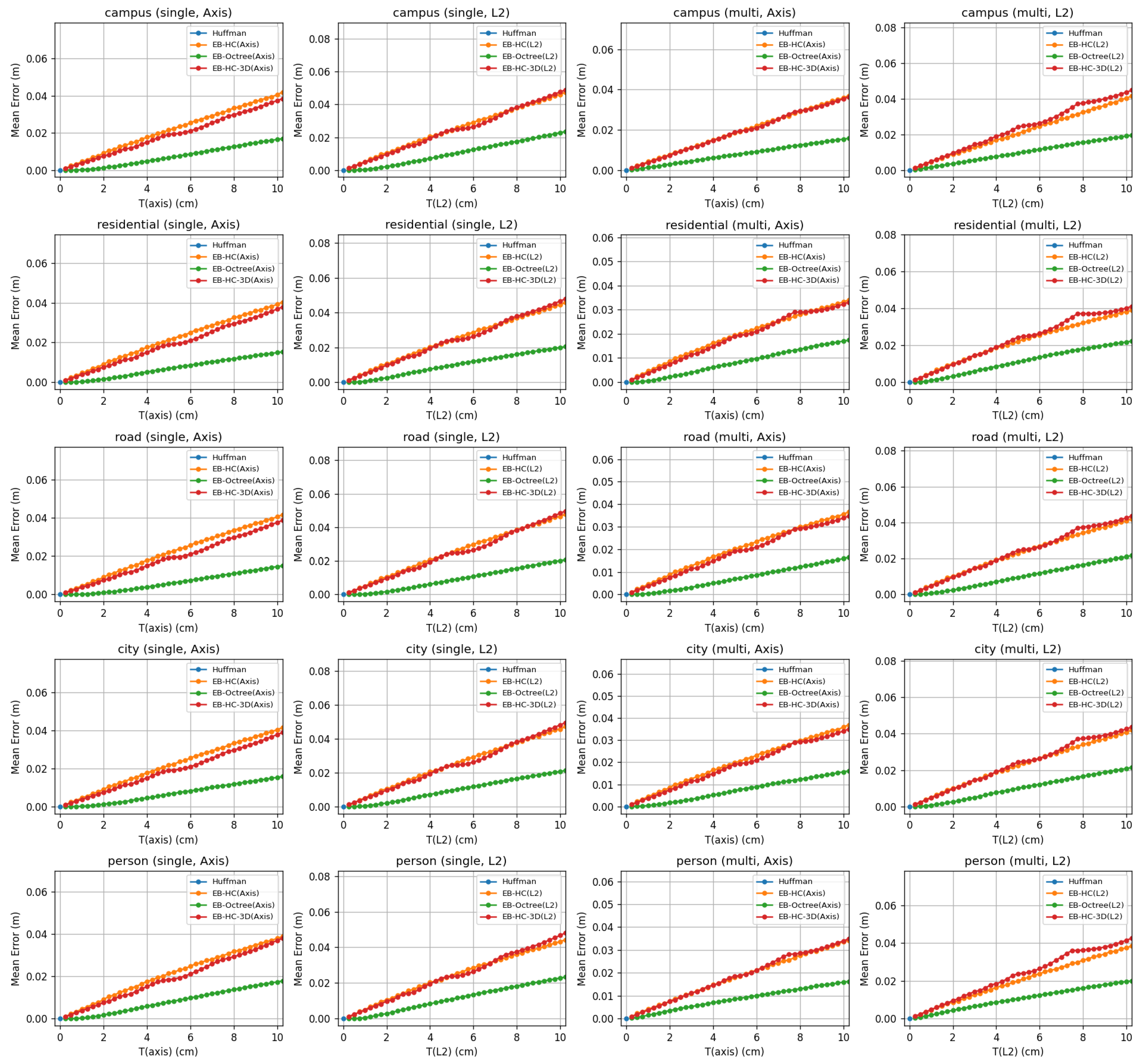
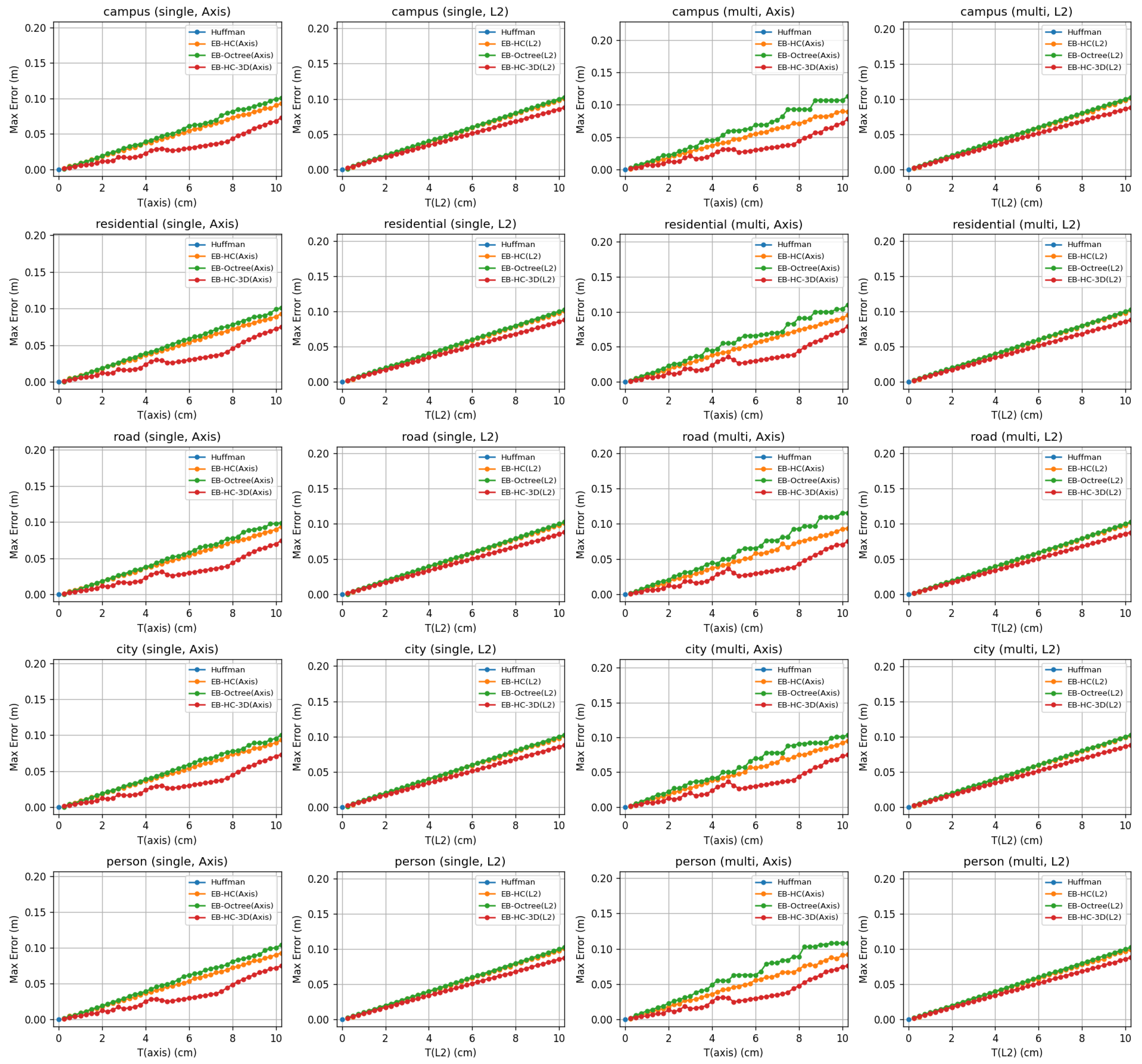
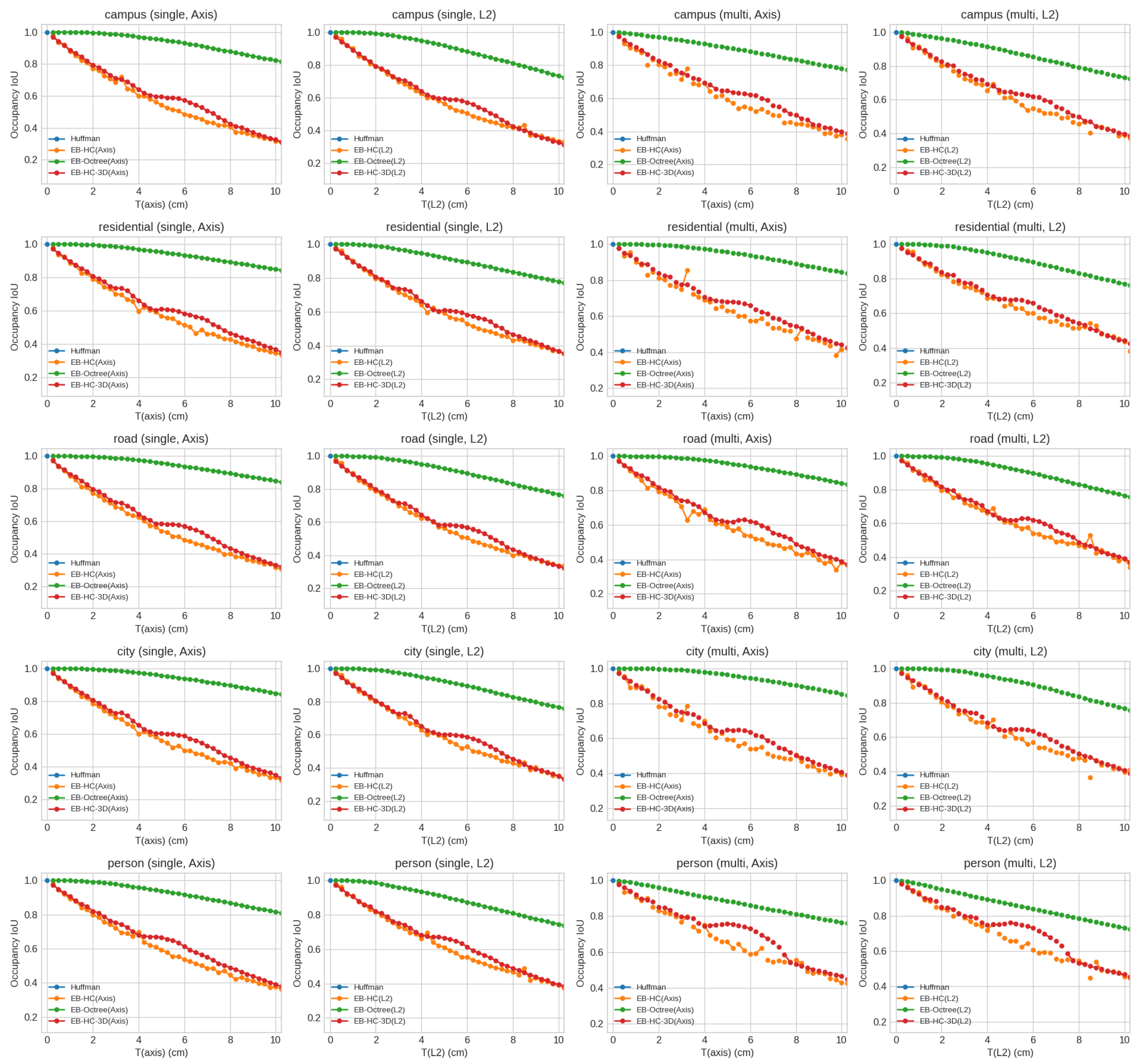
4.3. Comparison Among Compression Methods

In our experimental evaluation, we investigated the overall performance of our bounded-error compression framework by comparing the traditional lossless Huffman coding baseline with three families of bounded-error techniques (EB-HC, EB-3D, and the extended EB-HC-3D) implemented in two variants corresponding to either an axis-aligned (Axis) or an overall Euclidean (L2) error metric. The error threshold T varied from 0.25 cm to 10 cm. Because the LiDAR sensor’s inherent precision is approximately 2 cm, we report our results in two regimes: one with T ∈ [0.25, 2] cm that reflects the sensor’s accuracy, and another with T ∈ (2, 10] cm, where the allowed error exceeds the sensor precision.

Our experimental findings are further illustrated in Figure 1, Figure 2, Figure 3, Figure 4, Figure 5, Figure 6 and Figure 7. Figure 1 shows the combined compression ratio (CR) performance, demonstrating that the bounded-error methods can significantly reduce the data volume compared to the baseline, which consistently retains about 65% of the original data. Figure 2 presents the $t_{enc}$ performance, while Figure 3 compares the $t_{dec}$ across the different methods and error metrics. Figure 4 illustrates the mean reconstruction error across various scenes, demonstrating that the average error remains low. Figure 5 confirms that the maximum reconstruction error for all methods stays below the specified threshold T, thereby validating the fidelity constraints of our approach. Finally, Figure 6 and Figure 7 offer further insight into the geometric quality of the reconstructions by, respectively, analyzing the Chamfer Distance (CD) and the Occupancy Intersection over Union (IoU).

Under single-bin conditions, the baseline Huffman method consistently achieves a CR of roughly 0.65, meaning that about 65% of the original data volume is retained after compression, with extremely fast encoding and $t_{dec}$. In contrast, the bounded-error methods significantly reduce the data volume. When the error threshold is maintained within the [0.25, 2] cm range, the EB-HC variant (regardless of whether it uses an Axis or L2 metric) typically reduces the compressed data size to approximately 35% of the original. In these cases, encoding is completed in less than half a second and decoding takes only a fraction of a second. The extended EB-HC-3D method, which exploits three-dimensional correlations more aggressively, further reduces the CR to around 28%, although its decoding process is somewhat slower. Meanwhile, the EB-3D methods tend to retain a higher fraction of the original data (around 54–55%) in this low-threshold regime, as they prioritize lower computational complexity over maximum compression efficiency. Notably, while the mean reconstruction error for each method provides an indication of the average geometric deviation introduced during compression, all methods are designed so that their maximum error remains below the prescribed threshold T, thereby ensuring that the critical geometric fidelity is preserved.

As the permitted error increases beyond the sensor’s precision (with T ∈ [2, 10] cm), all bounded-error methods achieve even greater compression. In this higher-threshold regime, the EB-HC techniques typically achieve compression ratios near 28–29%, whereas the EB-HC-3D methods can compress the data to roughly 20%. The EB-3D variants, meanwhile, exhibit compression ratios in the low 40-percent range. Although processing times in this regime tend to be slightly reduced due to the relaxed error constraints, the overall trend is clear: higher allowed errors yield more aggressive compression.

When multiple bins are processed together, the performance trends observed in the single-bin tests are further enhanced by the exploitation of inter-bin correlations. In multi-bin experiments, the baseline Huffman method still delivers a CR of approximately 0.65; however, the bounded-error methods achieve even lower ratios. For instance, in a typical campus scenario with T ∈ [0.25, 2] cm, the EB-HC method compresses the data to about 35% of its original volume, with $t_{enc}$ on the order of 4 to 4.5 s and $t_{dec}$ approaching 1.7 s. Interestingly, in the multi-bin experiments for the Campus and Person scenes, the EB-3D methods (as implemented via the extended EB-HC-3D variant) yield better compression ratios than the corresponding EB-HC methods. This is likely because the point clouds in these scenes are relatively sparse and exhibit slow motion; as a result, consecutive bins show little change, making an octree-based subdivision approach particularly effective. In urban scenes, such as those found in the city dataset, the EB-3D method typically achieves compression ratios in the high 40-percent range with $t_{dec}$ of less than one second, while still maintaining competitive encoding performance.

For the low-error regime (T ∈ [0.25, 2] cm), which corresponds to the sensor’s inherent precision, the measured CD values are extremely low—often on the order of ${10}^{-6}$ or less. For instance, at (T = 0.25) cm the EB-HC methods achieve CD values of approximately $2.8\times {10}^{-6}$ in both Axis and L2 modes, while the EB-HC-3D variants report values of about $3.1\times {10}^{-6}$. This indicates that the reconstructed point clouds align extremely well with the ground-truth at the local scale. In this regime, the lossless baseline naturally yields an IoU of 1.0, and the bounded-error methods preserve nearly the entire volumetric occupancy.

At the borderline case of (T = 2) cm—the upper limit of the low-error regime—the performance of the different bounded-error methods begins to diverge. However, the local geometric fidelity, as measured by the Chamfer Distance, increases modestly to values on the order of $2.4\times {10}^{-4} \mathrm{t}\mathrm{o} 2.8\times {10}^{-4}$, reflecting the increased error allowance. In contrast, the EB-octree methods—which leverage octree subdivision to capture three-dimensional spatial correlations—exhibit CD values typically in the range of $1.5\times {10}^{-5} \mathrm{t}\mathrm{o} 3.3\times {10}^{-5}$ and maintain nearly perfect IoU values (close to 1.0 for the Axis variant and around 0.99 for the L2 variant). The extended EB-HC-3D methods fall between these two extremes, with CD values around $2.0\times {10}^{-4}$ and IoU values near 0.79. These differences at T = 2 cm underscore the trade-offs among the three methods in balancing local geometric detail against overall volumetric preservation.

In the high-error regime (T ∈ (2, 10] cm), the compression methods are allowed to be more aggressive. In this case, while the CD values increase modestly relative to the low-error regime—indicating that fine-scale geometric details are still largely maintained—the Occupancy IoU values vary considerably depending on the method. Methods that aim for maximum compression, such as the EB-HC variants, may experience a dramatic drop in IoU (to roughly 0.31–0.34), suggesting that a significant portion of the volumetric occupancy is lost or merged. In contrast, the extended EB-HC-3D variants tend to achieve intermediate IoU values (around 0.64), and the EB-octree methods—although slightly less aggressive in compression—excel at preserving volumetric fidelity, with IoU values ranging from about 0.77 up to nearly 1.0 at lower BE values, and around 0.84–0.87 at (T = 10) cm.

In summary, our results clearly demonstrate that by allowing a controlled error (quantified either as $e_{axis}\left(p,\widehat{p}\right)$ along individual axes or as $e_{L2}\left(p,\widehat{p}\right)$ in terms of the Euclidean norm), our bounded-error compression methods can dramatically reduce the storage requirements of LiDAR point clouds relative to the lossless Huffman baseline. Under single-bin conditions, when the error threshold is maintained within the sensor’s precision, our methods compress the data to roughly 25–35% of their original size. Multi-bin processing, which exploits temporal redundancies, enables some methods to achieve compression ratios as low as 15–25% of the original volume. Although multi-bin processing requires longer encoding (2.7 to 4.3 s) and $t_{dec}$ (0.6 to 3.5 s), the substantial reduction in data volume represents a significant benefit for applications such as autonomous driving, where both storage and transmission bandwidth are critical. Furthermore, the option to choose between Axis and L2 error metrics provides flexibility, with the L2 mode often yielding a modest gain in fidelity for isotropic point distributions. Importantly, across all methods and error settings, the maximum reconstruction error remains below the prescribed threshold T, ensuring that the geometric fidelity of the point clouds is consistently maintained.

This comprehensive analysis of CR, encoding/decoding times, reconstruction error, Chamfer Distance, and Occupancy IoU, evaluated across both low-error and high-error regimes, provides detailed guidance on the trade-offs inherent in each method. Such insights are essential for selecting an appropriate compression strategy based on the specific requirements for storage efficiency and geometric fidelity in practical applications.

4.4. Cloud-Edge Application Analysis

In a cloud-edge cooperative framework, the efficiency of onboard compression is vital not only for reducing storage and transmission bandwidth but also for meeting real-time processing demands. Our runtime evaluations were conducted on a 13th Gen Intel^® Core™ i7-13700K (Intel, Santa Clara, CA, USA) system using single-threaded execution (without GPU acceleration). Under these conditions, even the more sophisticated methods (such as the EB-HC-3D variants) exhibit performance that is encouraging for potential real-time applications.

We provide detailed profiling of compression and decompression runtime on a single-threaded Intel Core i7-13700K system. To illustrate, the lossless Huffman baseline compresses individual bin files in roughly 128 ms on average, while its decompression process takes around 353 ms. In comparison, the bounded-error methods require slightly longer processing times. For single-bin scenarios, the EB-HC method typically records an $t_{enc}$ of approximately 442 ms and a decoding time of about 187 ms, whereas the extended EB-HC-3D approach shows $t_{enc}$ near 525 ms and decoding times around 399 ms. These results illustrate how file size and error threshold affect runtime and demonstrate that parallelization or GPU acceleration can further reduce the computational overhead.

When we extend our experiments to multi-bin processing (where 10 consecutive bin files are handled together), the overall $t_{enc}$ is approximately 4.1 s for the EB-HC method and 3.1 s for the EB-HC-3D method. Although these aggregate times for 10 bins do not directly yield per-bin averages, they indicate that even under more demanding multi-bin scenarios, the processing durations remain within a range that suggests practical feasibility. It should be emphasized that these figures stem from our current, unoptimized, single-threaded implementation. There is significant potential for improvement through further algorithmic enhancements and code optimization, which could further diminish the computational overhead and better align the processing times with the strict real-time requirements of in-vehicle systems.

In conclusion, our current single-threaded implementation demonstrates that $t_{enc}$ for individual bin files varies from approximately 128 ms to 525 ms, while multi-bin experiments yield total $t_{enc}$ on the order of a few seconds. Although these processing times are not yet fully optimized for all real-time applications, the results are promising. With additional refinements and code optimizations, it is anticipated that the computational overhead can be further reduced, thereby meeting the real-time operational requirements essential for autonomous driving systems, where seamless coordination between onboard and cloud-based components is paramount.

5. Conclusions and Future Work

In this paper, we presented a bounded-error LiDAR compression framework that enforces a user-defined maximum coordinate deviation T, measured either in an axis-wise or Euclidean manner. By integrating clustering, hierarchical subdivision, and entropy coding, our approach reduces data volume to 25–35% for single-bin inputs and 15–25% for multi-bin configurations, all while rigorously constraining geometric errors. Notably, hierarchical subdivision enhances compression further, particularly in scenarios with sparse point distributions or overlapping bins. Evaluations on the KITTI dataset demonstrate that our method achieves an effective balance between data reduction and 3D fidelity, and runtime profiling indicates its potential for near real-time deployment in cloud-edge systems. Future work will investigate adaptive thresholding, parallel processing, and tighter integration with V2X communication to further optimize 3D perception pipelines for autonomous driving.

References

1. Chen, S.; Liu, B.; Feng, C.; Vallespi-Gonzalez, C.; Wellington, C. 3D point cloud processing and learning for autonomous driving: Impacting map creation, localization, and perception. IEEE Signal Process. Mag. 2020, 38, 68–86. [Google Scholar] [CrossRef]
2. Ayala, R.; Mohd, T.K. Sensors in autonomous vehicles: A survey. J. Auton. Veh. Syst. 2021, 1, 031003. [Google Scholar] [CrossRef]
3. Lo Bello, L.; Patti, G.; Leonardi, L. A perspective on ethernet in automotive communications—Current status and future trends. Appl. Sci. 2023, 13, 1278. [Google Scholar] [CrossRef]
4. Ahmed, M.; Mirza, M.A.; Raza, S.; Ahmad, H.; Xu, F.; Khan, W.U.; Lin, Q.; Han, Z. Vehicular communication network enabled CAV data offloading: A review. IEEE Trans. Intell. Transp. Syst. 2023, 24, 7869–7897. [Google Scholar] [CrossRef]
5. Arthurs, P.; Gillam, L.; Krause, P.; Wang, N.; Halder, K.; Mouzakitis, A. A taxonomy and survey of edge cloud computing for intelligent transportation systems and connected vehicles. IEEE Trans. Intell. Transp. Syst. 2021, 23, 6206–6221. [Google Scholar] [CrossRef]
6. Hasan, M.M.; Feng, H.; Hasan, M.T.; Gain, B.; Ullah, M.I.; Khan, S. Improved and Comparative End to End Delay Analysis in CBS and TAS using Data Compression for Time Sensitive Network. In Proceedings of the 2021 3rd International Conference on Applied Machine Learning (ICAML), Changsha, China, 23–25 July 2021; pp. 195–201. [Google Scholar]
7. Bandi, V.; Mahajan, N. Implementation of Compressed Point Cloud Streams in ROS; Technical Report, University of Texas at Austin: Austin, TX, USA. Available online: https://www.nalinmahajan.com/proj2/FRI_Final_Paper.pdf (accessed on 21 February 2025).
8. Abdelwahab, M.M.; El-Deeb, W.S.; Youssif, A.A. LiDAR data compression challenges and difficulties. In Proceedings of the 2019 5th International Conference on Frontiers of Signal Processing (ICFSP), Marseille, France, 18–20 September 2019; pp. 111–116. [Google Scholar]
9. Sun, X.; Luo, Q. Density-Based Geometry Compression for LiDAR Point Clouds. In Proceedings of the EDBT, Ioannina, Greece, 28–31 March 2023; pp. 378–390. [Google Scholar]
10. Liu, Y.; Tao, J.; He, B.; Zhang, Y.; Dai, W. Error analysis-based map compression for efficient 3-D lidar localization. IEEE Trans. Ind. Electron. 2022, 70, 10323–10332. [Google Scholar] [CrossRef]
11. Yoo, H.W.; Druml, N.; Brunner, D.; Schwarzl, C.; Thurner, T.; Hennecke, M.; Schitter, G. MEMS-based lidar for autonomous driving. e & i Elektrotechnik und Informationstechnik 2018, 34, 373–379. [Google Scholar] [CrossRef]
12. Dai, Z.; Li, Y.; Sundermeier, M.C.; Grabe, T.; Lachmayer, R. Lidars for Vehicles: From the Requirements to the Technical Evaluation; Institutionelles Repositorium der Leibniz Universität Hannover: Hannover, Germany, 2021. [Google Scholar]
13. Carthen, C.; Zaremehrjardi, A.; Le, V.; Cardillo, C.; Strachan, S.; Tavakkoli, A.; Dascalu, S.M.; Harris, F.C. A Spatial Data Pipeline for Streaming Smart City Data. In Proceedings of the 2024 IEEE/ACIS 22nd International Conference on Software Engineering Research, Management and Applications (SERA), Honolulu, HI, USA, 30 May–1 June 2024; pp. 267–272. [Google Scholar]
14. Yin, H.; Wang, Y.; Tang, L.; Ding, X.; Huang, S.; Xiong, R. 3d lidar map compression for efficient localization on resource constrained vehicles. IEEE Trans. Intell. Transp. Syst. 2020, 22, 837–852. [Google Scholar] [CrossRef]
15. Anand, B.; Kambhampaty, H.R.; Rajalakshmi, P. A novel real-time lidar data streaming framework. IEEE Sens. J. 2022, 22, 23476–23485. [Google Scholar] [CrossRef]
16. Mongus, D.; Žalik, B. Efficient method for lossless LIDAR data compression. Int. J. Remote Sens. 2011, 32, 2507–2518. [Google Scholar] [CrossRef]
17. Isenburg, M. LASzip: Lossless compression of LiDAR data. Photogramm. Eng. Remote Sens. 2013, 79, 209–217. [Google Scholar] [CrossRef]
18. Lipuš, B.; Žalik, B. Lossless progressive compression of LiDAR data using hierarchical grid level distribution. Remote Sens. Lett. 2015, 6, 190–198. [Google Scholar] [CrossRef]
19. Tu, C.; Takeuchi, E.; Carballo, A.; Takeda, K. Point cloud compression for 3d lidar sensor using recurrent neural network with residual blocks. In Proceedings of the 2019 International Conference on Robotics and Automation (ICRA), Montreal, QC, Canada, 20–24 May 2019; pp. 3274–3280. [Google Scholar]
20. Zhou, X.; Qi, C.R.; Zhou, Y.; Anguelov, D. Riddle: Lidar data compression with range image deep delta encoding. In Proceedings of the Proceedings of the IEEE/CVF Conference on Computer Vision and Pattern Recognition, New Orleans, LA, USA, 18–24 June 2022; pp. 17212–17221. [Google Scholar]
21. Anand, B.; Barsaiyan, V.; Senapati, M.; Rajalakshmi, P. Real time LiDAR point cloud compression and transmission for intelligent transportation system. In Proceedings of the 2019 IEEE 89th Vehicular Technology Conference (VTC2019-Spring), Kuala Lumpur, Malaysia, 28 April–1 May 2019; pp. 1–5. [Google Scholar]
22. Huang, L.; Wang, S.; Wong, K.; Liu, J.; Urtasun, R. Octsqueeze: Octree-structured entropy model for lidar compression. In Proceedings of the Proceedings of the IEEE/CVF Conference on Computer Vision and Pattern Recognition, Seattle, WA, USA, 14–19 June 2020; pp. 1313–1323. [Google Scholar]
23. Biswas, S.; Liu, J.; Wong, K.; Wang, S.; Urtasun, R. Muscle: Multi sweep compression of lidar using deep entropy models. Adv. Neural Inf. Process. Syst. 2020, 33, 22170–22181. [Google Scholar]
24. Wang, W.; Xu, Y.; Vishwanath, B.; Zhang, K.; Zhang, L. Improved Geometry Coding for Spinning LiDAR Point Cloud Compression. In Proceedings of the 2024 IEEE International Symposium on Circuits and Systems (ISCAS), Singapore, 19–22 May 2024; pp. 1–5. [Google Scholar]
25. Li, L.; Li, Z.; Liu, S.; Li, H. Frame-level rate control for geometry-based LiDAR point cloud compression. IEEE Trans. Multimed. 2022, 25, 3855–3867. [Google Scholar] [CrossRef]
26. He, Y.; Li, G.; Shao, Y.; Wang, J.; Chen, Y.; Liu, S. A point cloud compression framework via spherical projection. In Proceedings of the 2020 IEEE International Conference on Visual Communications and Image Processing (VCIP), Macau, China, 1–4 December 2020; pp. 62–65. [Google Scholar]
27. Varischio, A.; Mandruzzato, F.; Bullo, M.; Giordani, M.; Testolina, P.; Zorzi, M. Hybrid point cloud semantic compression for automotive sensors: A performance evaluation. In Proceedings of the ICC 2021-IEEE International Conference on Communications, Montreal, QC, Canada, 14–23 June 2021; pp. 1–6. [Google Scholar]
28. Chang, R.-I.; Chu, Y.-H.; Wei, L.-C.; Wang, C.-H. Bounded-error-pruned sensor data compression for energy-efficient IoT of environmental intelligence. Appl. Sci. 2020, 10, 6512. [Google Scholar] [CrossRef]
29. Chang, R.-I.; Li, M.-H.; Chuang, P.; Lin, J.-W. Bounded error data compression and aggregation in wireless sensor networks. In Smart Sensors Networks; Elsevier: Amsterdam, The Netherlands, 2017; pp. 143–157. [Google Scholar]
30. Chang, R.-I.; Tsai, J.-H.; Wang, C.-H. Edge computing of online bounded-error query for energy-efficient IoT sensors. Sensors 2022, 22, 4799. [Google Scholar] [CrossRef] [PubMed]
31. Geiger, A.; Lenz, P.; Stiller, C.; Urtasun, R. Vision meets robotics: The kitti dataset. Int. J. Robot. Res. 2013, 32, 1231–1237. [Google Scholar] [CrossRef]
32. Fan, H.; Su, H.; Guibas, L.J. A point set generation network for 3D object reconstruction from a single image. In Proceedings of the IEEE Conference on Computer Vision and Pattern Recognition (CVPR), Honolulu, HI, USA, 21–26 July 2017; pp. 605–613. [Google Scholar]
33. Mescheder, L.; Oechsle, M.; Niemeyer, M.; Nowozin, S.; Geiger, A. Occupancy Networks: Learning 3D Reconstruction in Function Space. In Proceedings of the IEEE/CVF Conference on Computer Vision and Pattern Recognition (CVPR), Long Beach, CA, USA, 16–20 June 2019; pp. 4460–4470. [Google Scholar]
34. He, Y.; Ren, X.; Tang, D.; Zhang, Y.; Xue, X.; Fu, Y. Density-preserving deep point cloud compression. In Proceedings of the IEEE/CVF Conference on Computer Vision and Pattern Recognition (CVPR), New Orleans, LA, USA, 19–24 June 2022; pp. 843–852. [Google Scholar]
35. Remelli, E.; Gojcic, Z.; Ortner, T.; Wieser, A.; Guibas, L.J.; Varanasi, K. Deep Implicit Moving Least-Squares Functions for 3D Reconstruction. arXiv 2021, arXiv:2103.12391. [Google Scholar]
Figure 1. Combined CR performance across multiple scenes.
Electronics 14 00908 g001
Figure 2. Combined t e n c performance across multiple scenes.
Electronics 14 00908 g002
Figure 3. Combined t d e c performance across multiple scenes.
Electronics 14 00908 g003
Figure 4. Combined mean reconstruction error analysis across multiple scenes.
Electronics 14 00908 g004
Figure 5. Combined maximum reconstruction error analysis across multiple scenes.
Electronics 14 00908 g005
Figure 6. Combined Chamfer Distance analysis across multiple scenes.
Electronics 14 00908 g006
Figure 7. Combined Occupancy IoU analysis across multiple scenes.
Electronics 14 00908 g007